Mad as Hell: Property Taxes and Financial Distress

Mad as Hell: Property Taxes and Financial Distress
                                                 Francis Wong∗

                                               October 29, 2020

                                                     Abstract

       Taxes on land and property are efficient in theory but uniquely unpopular in practice, and have
       been curtailed in 46 states. Unlike other taxes, property taxes may create financial distress when
       rising home values raise property tax bills but not incomes. I find that even modest tax hikes
       create distress: a $50 monthly tax hike increases mortgage delinquency by 9% and reduces auto
       consumption by $15. Homeowners report being able but unwilling to draw on housing wealth,
       and cite debt aversion as a key factor. Distortionary income-based relief reduces property tax
       animus, which is concentrated in counties that do not limit how much rising home values can
       raise property taxes. These findings suggest that financial distress makes efficient property
       taxation politically infeasible.

   ∗
    National Bureau of Economic Research. fwong@nber.org. I thank Emmanuel Saez, Amir Kermani, David
Sraer, and Danny Yagan for advice and encouragement. I also thank Alan Auerbach, Ingrid Haegele, Jonathan
Holmes, Paulo Issler, Peter Jones, Patrick Kline, Raymond Kluender, Julien Lafortune, Nicholas Li, Juliana Londono-
Velez, Neale Mahoney, David Schönholzer, Dmitry Taubinsky, Nancy Wallace, Wesley Yin, and numerous seminar
participants for helpful comments and discussions. This work was supported by the Lincoln Institute C. Lowell Harriss
Fellowship, the Fisher Center for Real Estate and Urban Economics, and the Russell Sage Foundation. Randomized
information treatments registered in AEA RCT Registry under identification number AEARCTR-0005784.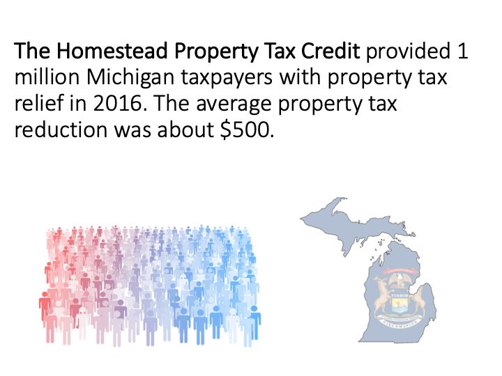

“Many people don’t understand that property taxes have absolutely no relation to a property owner’s
   ability to pay... those of us in the tax movement decided that our efforts must be directed toward
   bringing all taxes—but especially property taxes—down to a level where most people could pay them
   without undue hardship”

                          Howard Jarvis, progenitor of CA Proposition 13, I’m Mad as Hell (1979)

       Since the 19th century, influential economists have viewed taxes on land and immobile property
as more efficient than other forms of taxation (George 1879, Tiebout 1956).1 US property taxes
provide one-third (over $500 billion) of state and local government tax revenue and directly fund
many popular benefits such as public schools. Yet property taxes are America’s most despised tax.2
Starting with California’s 1978 tax revolt and passage of Proposition 13, 46 states have limited the
ability of local governments to tax property (Paquin 2015).3
       In public discourse, a common rationale for limiting property taxes is that property tax in-
creases, particularly those associated with rising home values, may occur even if homeowner income
remains unchanged. Consequently, property taxes can create financial distress among liquidity-
constrained homeowners. However, the idea that property taxes create financial distress is difficult
to reconcile with standard economic theories. Even in models in which moving houses is costly,
property taxes do not create financial distress because homeowners can convert housing wealth into
liquidity by borrowing against their homes.4
       This study is the first to simultaneously measure homeowner consumption, delinquency, and
borrowing responses to property taxes using high-frequency administrative data. Quasi-experiments
show that property tax hikes create financial distress. Homeowners do not borrow against their
homes to pay taxes, citing debt aversion as a key reason for not doing so. Survey experiments show
that income-based tax relief increases support for property taxes, suggesting that distortionary
modifications to pure property taxes may be needed to ensure their political sustainability.
       Guided by economic theory, research on property taxes has historically mostly ignored financial
distress. In addition, studies of homeowner responses to property taxes have faced two major
challenges. First, quasi-experimental variation in property tax liabilities tends to be small, limiting
the use of variation over time. Second, few data sources link outcomes measuring consumption and
financial distress to property tax liabilities at the individual level.
       This study overcomes those challenges by using quasi-experimental variation from property
reassessments in nine states between 2006 and 2015. Property reassessments are instances in which
   1
     Henry George viewed taxes on land as ideal because land is immobile capital. Moreover, taxes on land supposedly
encourage landlords to use the land for its most productive purpose (George 1879). Tiebout (1956) inspired the
subsequently prominent “benefit view”, which conceives of property taxes as producing no welfare costs because
homeowners can sort across jurisdictions to select their preferred bundle of taxes and amenities (Hamilton 1975).
   2
     Opinion surveys over the last fifty years have consistently shown that property taxes are more unpopular than
state and federal income, payroll, sales, and gasoline taxes (Cabral and Hoxby 2012).
   3
     Property tax limits often create severe revenue shortfalls: one estimate finds that California lost $30 billion in
2018 alone (Zillow 2018).
   4
     This is especially true when increases in property taxes are driven by increases in house price growth. This can be
seen in models that incorporate secured borrowing, house price growth, property taxes, and fixed costs from moving
(e.g. Kaplan et al. 2017).

                                                           1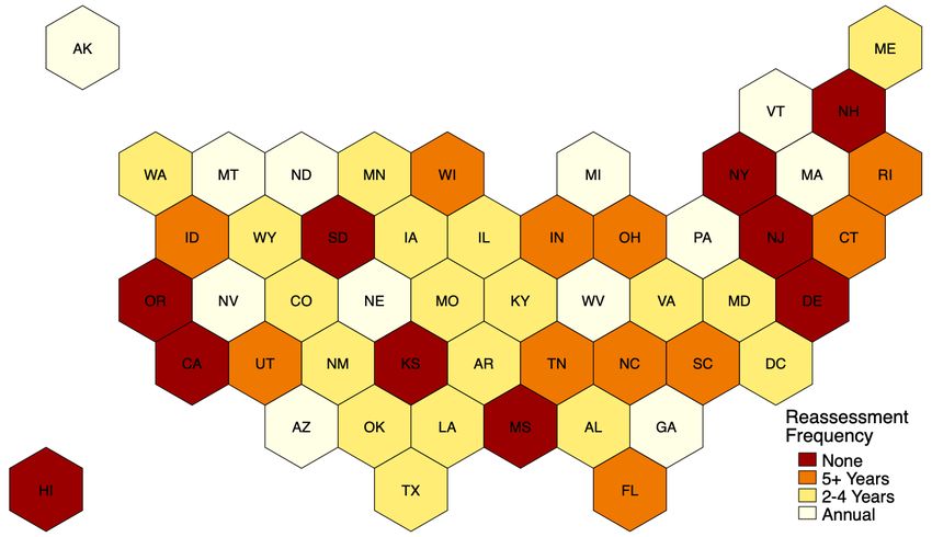

a local government updates the taxable value of property within its borders to reflect recent house
price growth. Most governments conduct reassessments at a less than annual frequency. These
infrequent reassessments can produce large changes to taxable property values and annual tax
bills. This study analyzes consumption, delinquency, and borrowing responses to property tax
increases by leveraging a novel data merge of credit bureau records, mortgage servicing records,
and local property tax records. Using the monthly servicing data, I am able to isolate the precise
month in which property tax payments increase for homeowners who pay their taxes in monthly
installments with their mortgage payments (about four in five homeowners with mortgages).
       I use an event study methodology to examine homeowner responses around the month that
property taxes increase. This approach assumes that homeowners with small increases in property
taxes and homeowners who have not yet experienced increases in property taxes represent a valid
counterfactual for the potential outcomes of homeowners with large increases in property taxes. I
find that a $50 increase in monthly tax payments generates a 9% increase in mortgage delinquency
and a reduction in auto consumption with a marginal propensity to consume of 0.31 after one year.
In theory, homeowners could draw on their housing wealth by taking out a second mortgage or
refinancing their existing mortgage; however, I find no adjustment on these margins. Surprisingly,
consumption responses are highest among homeowners with large amounts of housing wealth and
with high credit scores, suggesting that credit and liquidity constraints are not solely responsible
for the financial burden of property taxes. Effects on mortgage delinquency are strongest among
homeowners with less housing wealth and with lower credit scores.
       Why don’t homeowners draw on their housing wealth in response to property tax increases?
Even if property tax increases were not accompanied by increases in housing wealth, homeowners
should want to avoid delinquency.5 Standard economic reasoning suggests that financial frictions
(e.g. transaction costs, limited credit supply, or information frictions) may prevent homeowners
from borrowing against their housing wealth. However, it is difficult to rationalize the large con-
sumption responses exhibited by financially unconstrained homeowners with these frictions alone.
An alternative hypothesis is that homeowners may have a preference for avoiding additional in-
debtedness (i.e. debt aversion). I conduct a novel online survey of 3,000 US homeowners in order
to test this hypothesis. 77% of respondents say they would not take out a second mortgage even
if they had difficulty paying property taxes. The majority of those respondents (67%) would not
do so because they feel uncomfortable being in debt. A minority of respondents name transaction
costs (33%), credit supply (12%), or a lack of knowledge (4%) as reasons for not taking out a second
mortgage. These findings represent an important contribution of this study: preference-based debt
aversion is the key stated reason why homeowners do not draw on their housing wealth to pay their
property taxes.6
       Debt aversion also prevents homeowners from taking up a zero-interest loan to pay their property
   5
     Delinquency triggers a 5% late fee in most mortgage contracts, meaning that missing mortgage payments repre-
sents a very costly form of borrowing. Prolonged delinquency ultimately results in foreclosure and eviction.
   6
     Debt aversion is a very different explanation for homeowner illiquidity than those proposed in previous research,
which has typically focused on the role of large fixed costs (Chetty and Szeidl 2007, Kaplan and Violante 2014).

                                                          2

taxes. Property tax deferrals are a common form of tax relief which allow homeowners to postpone
paying property taxes (with interest) until they eventually transact their property. These policies
are theoretically appealing because they allow homeowners to avoid becoming liquidity constrained
without creating substantial economic inefficiencies. In the survey, 42% of respondents say that
they would never defer their property taxes, even at zero interest. 61% of those who would never
defer say that they would not want to feel like they were in debt, indicating that debt aversion is
a key deterrent to the effectiveness of tax deferrals. These results help explain the lack of success
of property tax deferral policies in the US. Thirty-one states offer taxpayers some form of property
tax deferral; however, even in places where eligibility criteria are broad, take-up of property tax
deferrals tends to be very low.7
       I use the survey of homeowners to explore policies that can make property taxes less unpopular
and find that aligning property taxes with homeowner incomes may substantially improve attitudes
towards property taxes. I conduct a randomized information treatment that informs respondents
in Michigan about their state’s income-based tax relief program. This policy lowers property taxes
for over one million taxpayers. Receiving randomized information about this policy reduces the
probability that a respondent identifies the property tax as the worst tax by 7 percentage points
(a 24 percent reduction). This finding supports the idea that financial distress among illiquid
homeowners generates animus towards property taxes. If this reduction were applied to nationwide
attitudes, the property tax would no longer be the most unpopular tax.
       The revealed links between property taxes, financial distress, and property tax animus help to
explain the historical unpopularity of property taxes. I show that enactments of statewide property
tax limits are concentrated in periods of rapid local house price growth. These are precisely the
circumstances under which illiquid homeowners would have experienced financial distress due to
the misalignment of property taxes and income flows. Moreover, survey data indicate that property
tax animus is concentrated in counties in which rapid house price growth led to higher property
tax burdens, but not in similar counties where local tax policies prevented house price growth from
increasing property taxes.
       An influential literature argues that property tax revolts such as Proposition 13 reflected the
desire of taxpayers to restrain government expenditures (Fischel 1989, Cutler et al. 1999). The
survey of homeowners does not point to a misalignment of voter preferences and the size of gov-
ernment revenues and expenditures as a contemporary contributor to homeowner animus towards
property taxes. Respondents appear to hold broadly positive attitudes towards local government.
Cabral and Hoxby (2012) argue that the salient nature of property taxes makes them particularly
painful compared to sales or income taxes. However, I find that property taxes cause financial
distress even among homeowners who pay property taxes in less-salient monthly installments.
       Studies of tax incidence in public economics rarely focus on financial distress. Economists have
debated the incidence of the property tax for decades, but financial distress is not represented in
   7
    For instance, the state of Washington offers a partial deferral of property taxes for homeowners with income less
than $57,000 as well as a full deferral for elderly individuals. In 2017, total take-up statewide was less than 600
households (Oline 2018).

                                                         3

most models of property tax incidence. The “benefit view” holds that property taxes do not incur
economic costs because households are mobile and value amenities funded by property taxes (Oates
1969, Hamilton 1975). In contrast, the “capital tax view” of property taxes identifies the existence
of efficiency losses due to capital flight (Mieszkowski 1972, Zodrow 2001, 2007), but financial distress
is not a source of inefficiency in this view. In both of these theories, the finding that property taxes
create financial distress is surprising and suggests unmodeled sources of inefficiency.
       Recent empirical studies have found evidence that property taxes meaningfully impact house-
hold finances, including impacts on labor supply (Shan 2010, Zhao and Burge 2017) and property
tax non-payment (Waldhart and Reschovsky 2012, Bradley 2013). Brockmeyer et al. (2020) find
that liquidity is an important factor mediating property tax compliance in Mexico City, and use
survey data to show that property tax hikes reduce consumption. Most relevant for this study, An-
derson and Dokko (2008) find that the timing of subprime borrowers’ first property tax bill impacts
mortgage delinquency, and Hayashi (forthcoming) finds evidence that tax cuts in Maryland during
the height of the Great Recession modestly reduced mortgage default filings against homeowners
and stimulated aggregate auto consumption.8 I use high-frequency data on mortgage payments
and a quasi-experimental research design validated by common trends to show that property tax
shocks have large impacts on mortgage delinquency and default.
       Property taxes are the predominant form of wealth taxation in the US. Wealth taxes have re-
ceived recent interest in policy circles (Sanders 2019, Warren 2019) and academic research (Seim
2017, Jakobsen et al. 2018, Avila and Londono-Velez 2019). Opponents of wealth taxation have
claimed that wealth taxes levied on both very wealthy and moderately wealthy individuals impose
heavy and unfair burdens on the latter group, whose assets are relatively illiquid (Sarin and Sum-
mers 2019, Saez and Zucman 2019). This study’s findings lend credence to the view that even
the moderately wealthy can experience financial distress from taxes on illiquid wealth. Hence,
sustaining a wealth tax may require exemptions for moderate levels of wealth or illiquid assets.9
       The remainder of this paper proceeds as follows. Section 1 provides institutional background on
property reassessments and property tax payments. Section 2 describes the dataset of merged credit
bureau, mortgage servicing, and property assessment records. Section 3 discusses the empirical
strategy. Section 4 presents the main empirical results. Section 5 presents results from the survey
of homeowners and discusses the debt aversion mechanism. Section 6 concludes.
   8
     My estimates of mortgage default are more than four times larger than those in Hayashi (forthcoming). Where
Hayashi measures mortgage default using legal filings initiated by lenders (a relatively imprecise measure of borrower
default), this study measures default using borrower payment decisions.
   9
     Indeed, recent wealth tax proposals (Sanders 2019, Warren 2019) have set very high exemption thresholds ($32
million and $50 million, respectively). Recent proposals for annual “mark-to-market” capital gains taxes have included
similar exemptions, such as requiring annual payments only on liquid-asset gains in the top 1% (e.g. Batchelder and
Kamin 2019).

                                                          4

1         Institutional Background
1.1        Property Reassessments
Property taxes in the US provide about one-third of state and local government tax revenue,
amounting to slightly more than $500 billion in 2016 (US Department of Commerce 2016b). Prop-
erty taxes also represent a large share of homeownership costs: in 2016, homeowners paid an average
of $3,000 in yearly property taxes (US Department of Commerce 2016b). One of the central chal-
lenges of property tax administration is repeatedly calculating the value of taxable property as
it changes over time, a process known as property assessment or reassessment. Most residential
property in the US is assessed by county or township governments under state-level policies that
regulate property assessment. Because of the costly and time-consuming nature of the assessment
process, most governments reassess property at a less than annual frequency.10
         I focus on large-scale property reassessments in nine states: Connecticut, Illinois, Indiana,
Missouri, New Hampshire, North Carolina, Ohio, Tennessee, and Washington. The goal of this
study is to analyze instances in which increases in house price growth generated large increases in
property tax liabilities. Each of these states conducted large-scale reassessments that are clearly
identifiable in the administrative data, and in which a large number of properties were reassessed
by local governments.
         Reassessment protocols vary greatly across these states. In Connecticut, North Carolina, Ohio,
and Tennessee (states that comprise 71% of the sample), property is assessed in regular cycles.
For instance, counties in Ohio reassess all residential property every six years (with reassessment
years varying by county). An example of this is shown in Figure 1, which illustrates the large
changes in both assessed values and tax bills during the 2012 reassessment in Cuyahoga County,
Ohio. Reassessments in the five states that do not adhere to regular cycles are more heterogeneous.
For example, Indiana underwent a significant reform of assessment practices in 2006, generating
large shifts in tax burdens due to reassessment. Appendix C contains a description of reassessment
practices in each state.11
         The main advantage of this setting is that it overcomes a common empirical challenge for
studying homeowner responses to property taxes, which is the relative stability of property taxes
over time in most other settings. Large-scale property reassessments offer ample variation in this
regard. A second advantage of this setting is that it abstracts away from changes in local government
revenues and expenditures. In other settings, increases in individual housing values and property
tax bills correspond to increases in total government revenues and consequently in the level of
    10
     Appendix Figure B1 illustrates the various frequencies at which local governments in the US are legally required
to reassess property.
  11
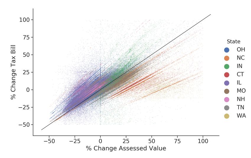
     The relationship between changes to assessed values and changes to property tax bills is positive and approxi-
mately linear. This relationship is not trivial. Hypothetically, if the value of all property within a jurisdiction were
increased by a similar amount, the jurisdiction could maintain tax bills fixed by reducing property tax rates. As
shown by example in Figure 1, this is often not the case due to substantial within-jurisdiction variation in house
price growth. The positive and linear relationship is illustrated in Appendix Figure B3, which provides a density
heat map of the relationship between changes to the tax bills and changes to assessed values for all properties in the
main analysis sample.

                                                           5

expenditures on local public amenities, but this is not generally the case for large-scale property
reassessments. Large-scale reassessments can create significant changes to individual assessed values
and tax bills without greatly affecting total tax revenues. For example, in Cuyahoga County in 2012
most homeowners experienced reductions to their assessed value; however, as shown in Figure 1 the
average change to property tax bills was close to zero. Because of the ability of local governments
to adjust property tax rates, total local government revenues can remain relatively stable despite
large changes to assessed values.

1.2      Property Tax Payments
Homeowners pay property taxes in one of two ways: directly to local taxing authorities (e.g. the
county) or through escrow accounts. Escrow accounts are typically maintained by mortgage ser-
vicers and allow homeowners to pay their property taxes, homeowner’s insurance, and mortgage
insurance in monthly installments together with their monthly mortgage principal and interest
payments. This offers homeowners the convenience of paying all of these expenses in one monthly
transaction. Mortgage servicers then pay property taxes to the government on behalf of the home-
owner. The share of mortgaged homeowners who pay property taxes in escrow has risen in recent
years, from 70% in 2011 to 79% in 2017 (Corelogic 2017).
      This study focuses on homeowners who pay property taxes through escrow accounts in order
to estimate a monthly event study around the month that taxes increase. For these homeown-
ers, I am able to isolate the timing of behavioral responses to property taxes, overcoming a key
challenge faced by previous studies. By law, mortgage servicers are required to conduct an escrow
analysis at least once a year. During an escrow analysis, servicers determine any account surplus
or shortfall associated with changing tax or insurance amounts. Servicers then adjust the monthly
escrow payment for the following twelve months accordingly. Because monthly escrow payments are
constant in the twelve months between escrow updates, for most borrowers there exists a specific
month in which the prior year’s property tax increase begins to be reflected in monthly property
tax payments. Consequently, I am able to estimate an event study around this same month.
      Estimating a monthly event study for homeowners who pay their property taxes directly to
the government is more challenging because it is harder to identify the exact month of the tax
increase. Homeowners receive notices of assessment as well as separate tax bills many months
before their tax bills are due. Moreover, tax bills often include secondary due dates. After the
first due date, homeowners can pay by a later due date with a late penalty.12 These considerations
complicate the expected timing of behavioral responses for homeowners paying property taxes
directly to local governments. While homeowners who pay property taxes through escrow accounts
also receive multiple notifications in advance of changes to their property taxes, the results in this
study demonstrate that the timing of the behavioral responses aligns with the month in which
property taxes are reflected in monthly escrow payments.
      Whether an individual pays their property taxes through an escrow account depends on both
 12
      For instance, taxpayers in California face a 10% penalty for delinquent property taxes.

                                                           6

lender-specific and borrower-specific factors. Homeowners without mortgages generally do not pay
property taxes through escrow accounts. Lenders are required to maintain escrow accounts for
certain loans with high loan-to-value ratios and interest rates (CFPB 2019). In other cases, lenders
may choose to offer escrow accounts. As discussed in Cabral and Hoxby (2012), this decision is likely
to depend on the profitability of offering borrowers access to escrow accounts, and by extension on
the extent of the lender’s existing servicing operations. In general, the requirement to pay property
taxes through an escrow account is a feature of mortgage contracts that is opaque to borrowers, and
information about escrow accounts tends to be revealed late in the process of securing a mortgage
(Cabral and Hoxby 2012). Particularly given the well-established lack of shopping across lenders
on behalf of mortgage borrowers, there is likely little systematic self-selection of borrowers into
mortgage contracts based on escrow requirements.13

2    Data
I analyze homeowner responses to property taxation by leveraging a novel data merge comprised of
three components: credit bureau records from Equifax, McDash mortgage servicing records from
Black Knight Financial Services, and property assessment and transaction records from ATTOM.
The Equifax and McDash data are also known as CRISM and cover approximately 60% of the US
mortgage market during the study period, 2005-2016. The Equifax credit bureau records contain
a number of individual-level attributes measured at the monthly level that are used by Equifax to
generate consumer credit reports. These data include information on both primary and secondary
mortgages, credit card utilization, auto loans, and loan delinquency. The McDash mortgage servic-
ing records contain loan-level characteristics such as original property value, original loan amount,
and loan type. These records also contain monthly loan information including payment status,
unpaid principal balance, principal and interest payment amounts, and escrow payment amounts.
Together, the data from Equifax and McDash capture a wide array of individual financial behaviors.
    The analysis relies on linking financial outcomes measured in CRISM with property tax liabilities
measured in the ATTOM property assessment and transaction records. The ATTOM data are
sourced from local property assessor and recorder offices and contain both annual property tax bills
and property assessments. Loans in CRISM are merged to properties in ATTOM using a k-nearest
neighbor algorithm which links records by original loan balances, property sale prices, and distress
events (e.g. foreclosures).14 This merge imbues observed annual property taxes and assessed values
(the two variables used in the analysis that are derived from the ATTOM data) with measurement
error. I discuss how I address the issue of measurement error in Section 3.
    The main analysis sample is comprised of primary mortgage loans in the nine sample states in
  13
     According to data from the National Survey of Mortgage Borrowers, almost half of borrowers only seriously
considered one lender before applying for a mortgage (Alexandrov and Koulayev 2018).
  14
     The transaction records from local recorder offices in ATTOM contain information on both sales and mortgages
associated with properties. This merge was conducted by the Fisher Center for Real Estate and Urban Economics
at the UC Berkeley Haas School of Business.

                                                       7

counties in which I observe the occurrence of a large-scale property reassessment.15 Within each
county, I restrict to observations in the highest tercile of merge quality associated with the k-nearest
neighbors algorithm, drop observations where the percent change in the property tax bill is outside
of -50% and 200%, and trim this variable at the 1% level. This process generates a sample of
261,577 unique loans across 10 reassessment years for a total of 299,545 loan-reassessment events.
         Table 1 provides summary statistics on the analysis sample. As a result of the reassessment
process, homeowners in the sample experience both large increases and decreases to their prop-
erty tax bills: the 10th and 90th percentiles correspond to a 14% decrease and a 20% increase,
respectively. When discussing results, I use “tax increases” as shorthand for “tax changes” since
regression coefficients are readily interpreted in terms of tax increases.

3         Empirical Strategy
The main empirical strategy centers around estimating a monthly event study around a property
tax increase. I focus on homeowners who pay property taxes through escrow accounts in order to
isolate the month in which escrow payments increase to reflect tax increases after reassessment.
Because escrow payment amounts are typically constant for twelve months following an annual
update, it is straightforward to identify the month in which payments increase to reflect a tax
increase.16
         In order to identify the causal impact of increases in property taxes paid through escrow ac-
counts, I use changes in annual property taxes measured in ATTOM as an instrument for changes
in monthly escrow payments. Note that if one were to use observed changes to escrow payments
alone, the estimates would be confounded by changes to insurance payments as well as property
taxes. However, under the assumption that changes in insurance payments are uncorrelated with
changes in property taxes due to reassessment, instrumenting with annual taxes isolates the causal
impact of tax increases on homeowner outcomes.17
         Formally, I estimate the causal impact of property taxes on homeowner outcomes using a two-
stage least squares (2SLS) regression, in which I instrument for the level change in the monthly
escrow payment using the percent change in the annual tax bill. The second stage is specified as:
                                                    X
                             yit = αi + γt,c(i) +           βk 1[t = ei + k](∆mi ) + εit                         (1)
                                                    k6=−2

Outcomes of interest for homeowner i in month t are given by yit . αi and γt,c(i) denote loan and
county-by-month fixed effects, respectively. ei denotes the month in which homeowner i experiences
a tax increase and ∆mi denotes the dollar change in the monthly escrow payment between k =
−2 and k = 1. Here, k = 0 corresponds to the month in which escrow accounts are updated
    15
     I describe the process used to verify the occurrence of large-scale reassessments in Appendix C.1.
    16
     See Appendix C.2 for a detailed explanation.
  17
     This is a natural assumption given that property tax increases are not generally included as a factor in setting
insurance premia.

                                                            8

to reflect property tax increases. I estimate Equation 1 by using {1[t = ei + k](∆Ti )}k6=−2 as
instruments for {1[t = ei + k](∆mi )}k6=−2 , where ∆Ti denotes the percentage change in property
taxes after reassessment.18 The estimation is conducted using a monthly panel of loans balanced
in k ∈ [−12, 11].19 Accordingly, I bin endpoints at k = −12 and k = 11 and cluster standard errors
at the loan level.
    The key assumption required to identify βk , the effect of a tax increase k months after the
increase occurs, is that the outcomes of homeowners with small increases in property taxes and
homeowners who have not yet experienced increases in property taxes represent a valid counter-
factual for the potential outcomes of homeowners who had large increases in property taxes. This
assumption can be validated by evaluating the presence of common trends (i.e. whether β̂k = 0 for
k < 0).
    Beyond isolating the impact of tax increases separately from other components of escrow pay-
ments, this specification carries two advantages. First, it circumvents the issue of measurement
error in ∆Ti , which is measured in the ATTOM data. With the exception of assessed values (which
are used as an alternative to tax bills in robustness analyses), the remainder of the variables in
Equation 1 do not carry measurement error from the data merge. Instrumenting with ∆Ti allows
βk to be interpreted without measurement error bias as the causal effect of a dollar increase in
property taxes. The second advantage of this approach is that for dollar-valued outcomes, βk can
be interpreted in terms of marginal propensities to consume and borrow.20
    The inclusion of county-by-month fixed effects restricts comparisons to homeowners within the
same county. In the context of reassessments, the vast majority of the variation in property taxes
within counties is driven by property reassessments rather than changes to tax rates. This can
be seen when comparing the variation in property taxes in a reassessment year to that outside
of a reassessment year (see Figure 1). The county-by-month fixed effects help to ensure that the
analysis compares homeowners living in the same area who experienced differential changes to
property assessments rather than differential changes in tax rates.
    The analysis focuses on four primary sets of outcomes. The first stage regression estimates
Equation 1 by OLS where the outcome is the dollar value of the monthly escrow payments. This
first stage regression validates that annual property tax increases result in monthly escrow payment
increases starting in the month of the escrow update. Second, I am interested in the consumption
response to increases in property taxes. In order to construct a measure of consumption, I follow
other studies that use credit bureau data (e.g. Di Maggio et al. 2017) and measure auto consump-
  18
     The distribution of level changes in annual property taxes is highly skewed because higher valued properties
experience larger level changes. Measuring ∆Ti in percentage terms better captures increases in property taxes that
represent meaningful shocks to homeowner finances, relative to measuring changes in property taxes in dollar terms.
The main advantage of measuring ∆mi in dollar terms is that it allows βk to be interpreted in terms of marginal
propensities to consume and borrow, simplifying the interpretation of the estimated coefficients.
  19
     See Appendix C for more details on the construction of the monthly panel.
  20
     An alternative approach would be to estimate a reduced form version of Equation 1 by OLS, using ∆Ti as the
main regressor. I discuss the results of this exercise in the following section, which show that the results are unchanged
when scaling the estimated coefficients by the first stage and that the 2SLS strategy scales effect sizes to net out
measurement error.

                                                            9

tion as the difference in total auto balances between any two months in which auto balances increase
by more than $5,000. This approach to measuring auto consumption assumes that a one-month
increase in auto loan indebtedness of more than $5,000 represents the purchase of a new car.
       Third, I evaluate the effects of property tax payments on mortgage delinquency and mortgage
default. I define an indicator for mortgage delinquency that takes a value of 1 if the mortgage is
thirty or more days past due and 0 if the mortgage is current. To measure mortgage default, I
define an indicator that takes a value of 1 if the mortgage is ninety or more days past due and 0
otherwise. The distinction between mortgage delinquency and default is an important one. In the
data, only a small minority (16%) of loans that are thirty days delinquent transition into deeper
delinquency the following month, while almost half (47%) of loans that are ninety days delinquent
transition into deeper delinquency or foreclosure.21
       Fourth, I measure the response of home equity extraction to changes in property tax burdens.
Homeowners can convert their housing wealth into liquidity through two types of loans. The first
type is a junior-lien mortgage, which includes closed-end second mortgages and home equity lines
of credit (HELOCs). Closed-end second mortgages offer borrowers a fixed amount of credit while
HELOCs offer a rotating line of credit. Junior-lien mortgages are taken in tandem with primary
mortgages and are backed by the borrower’s property but carry a lien on the property that is
subordinate to that of the primary mortgage. In order to measure conversion of housing wealth
into liquidity through junior-lien mortgages, I define a variable that captures the total monthly
balance of both closed-end second mortgages and HELOCs. The second type of loan is a cash-out
refinance loan. Cash-out refinances allow borrowers to refinance their primary mortgage and to
borrow more than the outstanding balance of the original loan. To capture cash-out refinances, I
define a variable that measures the total monthly balance of primary mortgages.22
       Secondary outcomes include credit card borrowing and non-mortgage delinquency. These rep-
resent alternative margins of adjustment for homeowners. I measure credit card borrowing using
the dollar value of current credit card balances. Because homeowners could hypothetically generate
liquidity by going delinquent on a wide range of loans, I measure non-mortgage default using the
dollar value of non-mortgage accounts that are thirty or more days past due.23
  21
      Appendix Table A2 presents a transition matrix of mortgage payment statuses from the analysis sample.
  22
      The Equifax data follow borrower outcomes for six months after the mortgage loan (measured in McDash) has
been paid off or transferred to another servicer. This allows the total monthly balance of primary mortgages to
capture new balances of refinanced loans. This unique feature of the data also helps to address the issue of attrition.
Mortgages that are paid off or transferred attrit from the sample during the observation window. Properly evaluating
the presence of common trends in Equation 1 requires not conditioning the sample on mortgages that survive until
an escrow update around k = 0. For this reason, I code all flow outcomes (e.g. delinquency, auto consumption) as
zero if missing and forward fill all stock outcomes (e.g. mortgage balances). To evaluate robustness to these choices,
I estimate Equation 1 on a sample of mortgages that are open throughout the observation period. The results of this
exercise are presented in Appendix Figure B5 and show that the estimated responses are unaffected.
   23
      Non-mortgage accounts include both loans and other accounts in collections. I winsorize all dollar-valued out-
comes measured in the credit bureau data at the 99th percentile of positive values.

                                                          10

4     Results
This section presents estimates from the event study specification in Equation 1. Figure 2, panel
A plots the first stage regression, in which the main outcome variable is the dollar amount of
monthly escrow payments. I estimate Equation 1 by OLS and scale ∆Ti by the mean property
tax bill before reassessment ($2,893). This scaling allows the coefficients to be interpreted as the
effect of a $1 increase in property taxes on the monthly escrow payment. Panel A shows that this
design precisely identifies the month in which monthly escrow payments are updated to reflect new
property tax payments, corresponding to event time k = 0. A $1 increase in the annual property
tax bill measured in the ATTOM data corresponds to an increase of about $0.052 per month in
escrow payments measured in the McDash data (corresponding to a $0.629 yearly increase).
    These estimates imply that monthly escrow payments only increase 63% as much as they would
if increases in property taxes were passed through dollar for dollar into increases in escrow payments.
The primary reason for this is measurement error in ∆Ti , which naturally reduces the size of the
estimated coefficient. A secondary factor may be that mortgage servicers maintain some extra
balance in escrow accounts as a cushion against fluctuations in homeownership expenses. Servicers
may adjust the size of this cushion in response to changes in property tax bills. If this is the
case, property taxes may not pass through into escrow payments dollar-for-dollar. These issues
are circumvented by estimating Equation 1 by 2SLS using the percent change in the property
tax bill (∆Ti ) as an instrument for the change in the monthly mortgage payment (∆mi ). This
specification allows the coefficients to be interpreted as the causal effect of property tax increases
without measurement error bias.

4.1    Consumption
Homeowners substantially reduce auto consumption after a property tax increase. Figure 2, panel B
plots event study coefficients estimated by 2SLS, where the outcome is the twelve-month cumulative
sum of auto consumption. These estimates imply that a $1 increase in monthly escrow payments
reduces auto consumption by about $3.38 after 11 months, corresponding to an MPC of 0.31. The
flat trend in auto consumption leading up to the event month validates the identification assumption
and supports a causal interpretation of the relationship between increases in property taxes and the
observed responses. The estimates are between the large auto MPC of 0.48 measured in response
to stimulus payments (Parker et al. 2013) and the relatively smaller auto MPC of 0.08 found in
the context of adjustable rate mortgage resets (Di Maggio et al. 2017).24
    The lack of anticipatory behavior is surprising. Even though mortgage servicers pay property
taxes on behalf of the homeowner, local governments send homeowners both a notice of assessment
and a tax bill each year many months in advance of the property tax due date. It is therefore
  24
     Hayashi (forthcoming) finds that a $1,000 reduction in median property taxes from 2008 to 2009 increases ZIP-
level car purchases by 10%. Comparing our estimates is somewhat challenging in light of my result that consumption
responses occur only after a payment increase. This implies that some of the ZIP-level response may have occurred
outside of the measurement window.

                                                       11

puzzling that homeowners only appear to cut consumption when they face monthly payment in-
creases, suggesting that homeowners who pay property taxes through escrow accounts are highly
inattentive to changes in property tax liabilities.
   An important distinction between the results in this study and those measured in the context
of changes to mortgage payments is that the cost increases in this study should correspond to
increases in home values. Given tax rates on the order of 1%, increases in housing wealth are large
relative to the resulting tax increases. The observed consumption responses imply that homeowners
who have experienced increases in the value of their homes and comparatively small increases in
their tax liabilities respond to the tax increases by reducing car purchases. Thus, despite a net
increase in wealth, homeowners appear to respond strongly to changes in liquidity. This finding
echoes results from studies of consumption responses to changes in housing and liquid wealth.
Estimates of consumption and borrowing responses to liquid wealth (e.g. Johnson et al. 2006,
Parker et al. 2013) tend to be substantially larger than responses to housing wealth (e.g. Mian
and Sufi 2011, Mian et al. 2013, Cloyne et al. 2019). This pattern is at odds with theoretical
predictions suggesting that responses to the two types of shocks should be more similar than is
typically observed (Berger et al. 2017). The empirical responses suggest the presence of important
frictions that prevent homeowners from consuming out of their housing wealth.

4.2   Financial Distress
Property tax hikes also appear to create financial distress: the estimates presented in Figure 3 indi-
cate higher rates of mortgage delinquency and mortgage default following a property tax increase.
The coefficients are scaled to reflect effects relative to a $100 increase in monthly mortgage pay-
ments. Figure 3, panel A demonstrates an immediate increase in mortgage delinquency following
increases in monthly mortgage payments. Relative to the pre-event mean, a $100 monthly payment
increase results in a 10% increase in delinquency the month after the payment increase, and an
18% increase after 11 months. Panel B illustrates that increases in mortgage default manifest more
gradually. A $100 payment increase translates into a 30% increase in mortgage default relative to
the pre-event mean of 1.4%.
   Even if property tax increases were not accompanied by increased housing wealth, homeowners
should still be willing to incur substantial costs to avoid delinquency and default. This is because
missing mortgage payments is a costly decision: missed payments usually carry a 5% late fee as well
as negative impacts on credit scores. Prolonged delinquency will ultimately result in foreclosure
and eviction. Importantly, the effects on mortgage delinquency persist for many months without
signs of reverting to pre-event levels. If homeowners were simply forgetting to maintain sufficient
balance in their checking accounts in the month of the update but were to adjust their finances
appropriately upon noticing the change, these effects would disappear in the months following the
update; however, the event study coefficients indicate persistent increases in delinquency. These
results provide direct evidence that property taxes generate financial distress among homeowners.
   Strikingly, my estimates of mortgage default are more than four times larger than those found

                                                  12

in Hayashi (forthcoming), who measures mortgage default using legal filings initiated by lenders
against delinquent borrowers. This measure of default may be subject to significant attenuation bias
because it captures the decisions of lenders rather than borrowers, and filings do not mechanically
follow borrower default. My default estimates are about twice as large as those found in Fuster
and Willen (2017) who use data similar to those in this study to analyze the relationship between
mortgage default and payment size in the particular context of adjustable rate mortgage resets.
       The estimated magnitudes are particularly striking given that the increases in monthly payments
are modest. Table 1 shows that the 90th percentile of property tax increases corresponds to a 20%
annual increase. Scaled by the average tax bill, this amounts to a $50 monthly increase in tax
payments. Therefore, the observed effects on financial distress (e.g. a 9% increase in mortgage
delinquency for a $50 increase) are generated by very small shocks to housing costs, suggesting a
high degree of financial fragility among homeowners. These results are consistent with other work
showing that many Americans are exceedingly vulnerable to small shocks (Mello 2018).

4.3      Converting Housing Wealth into Liquidity
In theory, homeowners experiencing increases in home values and property tax liabilities could nat-
urally adjust by converting housing wealth into liquidity through home equity extraction; however,
homeowners do not appear to adjust along this margin. Figure 4 plots the event study results for
home equity extraction. Panel A plots effects on second (i.e. junior-lien) mortgage balances, while
panel B plots effects on first (i.e. primary) mortgage balances. If homeowners were to draw on their
housing wealth in order to pay higher property tax bills, one would expect to see first and second
mortgage balances increase; however, this behavior is absent. The confidence intervals for second
mortgage balances in panel A reject large marginal propensities to borrow. First mortgage balances
are substantially noisier; however, the pattern is stable over time and loan balances show no signs
of increasing. These results indicate that in response to property tax increases, homeowners reduce
consumption and are more likely to miss mortgage payments, but do not draw on their housing
wealth in order to pay taxes.
       In additional results, I find no evidence of significant adjustment using credit cards or delin-
quency on non-mortgage accounts. These results are presented in Appendix Figure B4. While there
is some indication that delinquent non-mortgage account balances increase, the estimated increase
is quantitatively small relative to the reduction in auto consumption and statistically insignificant
in most months. The estimated increase in the current balance of credit cards is also quantitatively
small, and de-trending the balance of credit cards over this time horizon suggests no significant
adjustment. Moreover, if homeowners were coping with tax increases using credit cards, one would
expect a sharp increase in credit card balances immediately following the tax increase, but credit
card balances trend smoothly throughout the event month.25
       An important outstanding question is the extent to which the observed consumption, delin-
  25
    While a sharp increase in credit card borrowing (rolled-over balances) could hypothetically be offset by a sharp
reduction in consumption (non-rolled-over balances), this is unlikely given the lack of a trend break in either direction.

                                                           13

quency, and borrowing responses apply to homeowners who pay property taxes directly to local
governments. Homeowners without mortgages generally pay in lump sum, often in biannual or
quarterly installments. This group includes many elderly homeowners, who may be particularly
financially vulnerable to increases in homeownership costs. Without escrow accounts, tax increases
are not mechanically smoothed over the course of twelve months, so property taxes may create even
more financial strain for these homeowners. While evaluating this possibility is of independent in-
terest, the challenges in measuring the timing of tax increases for homeowners paying in lump sum
make this empirical setting unlikely to yield accurate comparisons between the two groups.

4.4      Robustness
An important consideration for interpreting homeowner responses to property taxes is the extent to
which increases in property taxes correspond to house price growth. If increases in property taxes
are not correlated with higher home values, it would be less surprising that increases in property
taxes generate reductions in consumption. Changes in mortgage payments have been observed to
reduce consumption and increase delinquency in other settings (Di Maggio et al. 2017). In the
sample states, reassessments are designed to align assessed values with market values, meaning that
changes in assessed values typically reflect changes to market values. In Column 1 of Table 2, I
find the same consumption and mortgage delinquency patterns when examining the direct effects
of changes to property assessments instead of property taxes.26
       A curious feature of the reassessments in many of the sample states is that despite statutory
requirements to do so, many properties are not reassessed when they are transacted, raising the
possibility that the observed responses might be driven by new homeowners who have not benefited
from recent house price growth. Moreover, studies have found evidence that new homebuyers are
inattentive to changes in property assessments (Bradley 2017). I address this concern in Column
2, where I restrict to homeowners that have lived in their houses for at least four years at the
time that their monthly tax payments increase. These homeowners display similar patterns. In
Column 3, I restrict the sample to the four states in the sample that conduct reassessments through
regular cycles: Ohio, North Carolina, Tennessee, and Connecticut. Interestingly, while the effects
on consumption are similar to other specifications, the negative impacts on mortgage delinquency
and default disappear, suggesting that that there may be significant benefits to maintaining highly
predictable reassessment protocols.
       The main sample spans the Great Recession, a time in which many homeowners were financially
distressed and in many cases underwater on their homes. This period was also characterized by
contractions in credit supply. One potential concern is that property taxes only cause distress
when credit access is low and house values are declining. In Column 4 of Table 2, I restrict the
  26
    Note that even if inaccuracies in property reassessments exacerbate tax burdens, property taxes nonetheless ap-
pear to impose financial distress on homeowners. Reassessments are necessary in order to avoid very large distortions
to the tax base over time. Moreover, as discussed later in this section when examining heterogeneous responses,
even homeowners with access to cheaper means of borrowing exhibit increased rates of mortgage delinquency. This
suggests that the financial distress created by property taxes is not merely a product of imperfect measurement of
property values or financial constraints, but also of behavioral frictions. These are explored in Section 5.

                                                         14

sample to properties that were reassessed in or after 2011. Homeowners exhibit similar consumption
responses outside of the Recession. While the effects on loan default are smaller and less significant,
commensurate with elevated rates of mortgage default during the Great Recession, the effects
on loan delinquency remain large and significant. This result implies that property taxes create
meaningful financial distress even in normal times.
   Lastly, I address potential econometric concerns associated with estimating Equation 1 by
2SLS. One potential issue is that the endogenous variable (monthly escrow payments) is not well-
measured for loans that are paid off or refinanced before the month of the scheduled tax increase.
Accordingly, I estimate Equation 1 by OLS, interacting the percent change in the tax bill with
event time indicators. Appendix Figure B6 shows that the OLS estimates yield results that are
very similar to the 2SLS specification.

4.5   Heterogeneity
The preceding results show that in response to property tax increases, homeowners reduce con-
sumption and are more likely to miss mortgage payments, but do not draw on their housing wealth
in order to pay property taxes. This suggests the existence of frictions that prevent homeowners
from converting housing wealth into liquidity. In theory, homeowners may be prevented from draw-
ing on housing wealth due to preference-based factors (e.g. debt aversion) or financial constraints.
Recent work in economics has largely focused on the latter, typically in the form of fixed costs
associated with drawing on housing wealth (Chetty and Szeidl 2007, Kaplan and Violante 2014).
In addition, credit supply frictions may prevent homeowners from qualifying for the loans required
to draw on housing wealth, or they may lack the knowledge to do so (i.e. information frictions).
This section will explore heterogeneous responses that help to distinguish between these potential
explanations.
   Evaluating heterogeneous responses is informative about the extent to which housing wealth,
credit access, and liquidity can explain the observed responses. Table 3 provides estimates of β10
from Equation 1 (i.e. effects after 11 months) broken down by subgroups. Columns 1 and 2 split the
sample of homeowners by amount of housing wealth. High-housing wealth homeowners are defined
as those with a pre-event combined loan-to-value ratio of below 80%. Interestingly, the estimated
consumption effects for high-wealth homeowners are large and statistically significant. Moreover,
the magnitude of the responses is statistically indistinguishable from that of low-wealth homeown-
ers. The point estimates even suggest slightly larger responses for high-wealth homeowners: the
estimated MPCs for high- and low-wealth homeowners are 0.42 and 0.24, respectively. Importantly,
these differences are not driven by higher levels of consumption among high-wealth households. On
the contrary, annual auto consumption appears to be about 25% smaller than that of low-wealth
households, implying higher elasticities for high-wealth households. Less surprisingly, high-wealth
homeowners exhibit somewhat more moderate delinquency responses, although default responses
are similar in magnitude and statistically indistinguishable.
   Similarly, homeowners with higher credit scores (and therefore more access to credit) exhibit

                                                  15

large consumption reductions in response to tax increases. Columns 3 and 4 of Table 3 present
results split by credit score. Prime and sub-prime borrowers exhibit MPCs of 0.31 and 0.28, respec-
tively.27 Part of this difference may be due to the leveraged nature of auto consumption observed
in the data (i.e. prime borrowers may have more access to auto loans). As with high-wealth home-
owners, it is striking that responses for both groups are large and statistically indistinguishable.
The delinquency and default responses are concentrated among subprime borrowers, a result that
is unsurprising given that credit scores are designed to identify borrowers least likely to default.
       Even homeowners who have the ability to borrow using credit cards appear to become financially
distressed as a result of property tax increases. Column 5 restricts the sample to homeowners with
open credit cards with less than 50% total utilization and more than $500 in unused credit limits
while Column 6 restricts the sample to homeowners with more than 50% utilization or less than
$500 in unused credit limits. Homeowners with the ability to borrow on their credit cards exhibit
higher rates of mortgage delinquency after a tax increase. This is particularly significant because
the 5% late fees associated with late mortgage payments imply that delinquency represents a much
more costly form of borrowing (i.e. one with a 60% APR) than credit card borrowing.28
       The finding that even homeowners who do not appear to be financially constrained exhibit strong
consumption and delinquency responses to tax increases is surprising and implies that the financial
burden of property taxes cannot be explained by financial constraints alone. This motivates an
exploration of non-financial explanations for why homeowners do not draw on their housing wealth
or on existing borrowing capacity. The likely importance of non-financial factors is supported by
findings in Kueng (2018) and Olaffson and Pagel (2018) that show that even highly liquid individuals
display large consumption responses to predictable income shocks. These studies both find that
liquidity constraints alone cannot rationalize large consumption responses, suggesting behavioral
explanations for these patterns. Similarly, Chetty et al. (2014) demonstrate that a large share of
individuals appear to use cash-on-hand as a rule of thumb for making consumption decisions. The
following section presents evidence from a survey of US homeowners indicating that preference-
based debt aversion is a key factor determining homeowner responses to property taxes, which
helps explain the large responses to property taxes exhibited by homeowners who do not appear to
be financially constrained.
  27
      Prime borrowers are defined as those with a VantageScore 3.0 of 660 or greater. VantageScore 3.0 is designed
to correspond closely to the well-known FICO credit score. Both scores range from 300 to 850, with 660 being an
approximate cutoff for prime borrowers.
   28
      In supplementary analyses, I split the sample based on two additional proxies for liquidity. The first liquidity proxy
is back-end debt-to-income ratio at loan origination (DTI). DTI measures a borrower’s total monthly debt payments
relative to a borrower’s total monthly income. The results are similar to those in the main heterogeneity analysis:
even liquid homeowners experience impacts on consumption and financial distress. Second, I restrict the sample
to homeowners with a home equity line of credit. These homeowners should have extremely liquid wealth because
they have already established a revolving credit line secured by their housing wealth. I find no significant effects of
property tax increases on consumption, delinquency, and default for these homeowners. While this may suggest that
a small share of homeowners that are willing and able to extract home equity do not experience financial hardship as
a result of property tax increases, this result must be interpreted with caution given that these homeowners represent
only about 15% of the sample and thus these responses are estimated imprecisely. The results of this supplementary
analysis are presented in Appendix Table A3.

                                                            16