MAGNETISMO CROSTALE: ESEMPI, AEROMAGNETISMO, SATELLITI PER MAGNETISMO E MAGNETSMO DEI PIANETI - Antonio Meloni Per studenti di Geofisica Generale ...
←
→
Page content transcription
If your browser does not render page correctly, please read the page content below
MAGNETISMO CROSTALE: ESEMPI,
AEROMAGNETISMO, SATELLITI PER MAGNETISMO
        E MAGNETSMO DEI PIANETI

                  Antonio Meloni
  Per studenti di Geofisica Generale ed Applicata

            Univ. Roma Tre, 2012-2013

                    (47 pagine)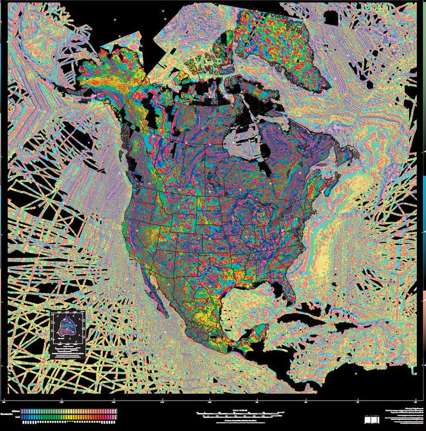
Magnetic anomaly data provide a means of “seeing through”
nonmagnetic rocks and cover such as vegetation, soil, desert sands,
glacial till, man-made features, and water to reveal lithologic varia-
tions and structural features such as faults, folds, and dikes.

Magnetic anomalies reflect variations in the distribution and type of
magnetic minerals—primarily magnetite—in the Earth’s crust. Magnetic
rock can be mapped from the surface to great depths, depending on their
dimensions, shape, and magnetic properties, and on the character
of the local geothermal gradient.

In many cases, examination of magnetic anomalies provides the most
expeditious and cost-effective means to accurately map geologic features
in the third dimension (depth) at a range of scales.
INDAGINI MAGNETICHE IN ITALIA. Il RILIEVO A TERRA DEL PFG

                                   More than 2700 stations to produce
                                   a secular variation model and
                                   magnetic maps of the total intensity
                                   (F), the vertical component (Z), and
                                   the horizontal component (H) of the
                                   Earth’s magnetic field.

                                   Moreover in the period 1965 – 1972,
                                   oceanographic campaigns were
                                   promoted by the (CNR) in the
                                   Mediterranean Sea. The cruises
                                   were performed by the Osservatorio
                                   Geofisico Sperimentale (OGS). The
                                   ship Bannock was employed for this
                                   purpose until 1971, then replaced by
                                   the ship Marsili. A proton precession
                                   magnetometer was used to carry out
                                   measurements of the total intensity
                                   of the Earth’s magnetic field; its
                                   sensor was placed in a towed fish at
                                   200–300 m from the ship,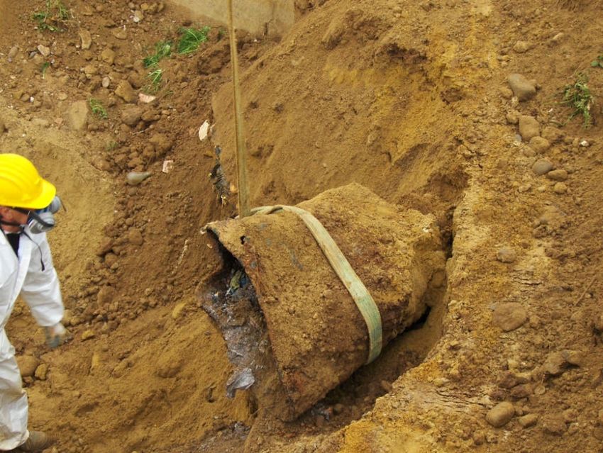
The most remarkable result of this
new map, with respect to the
previous, is an unprecedented view
of the magnetic anomaly field of the
whole area at ground level, which
contains many imprints of the major
tectonic elements of Italy, and
portrays their regional
characterization. The obtained
magnetic anomalies correlate with
many of the structural features
known in the area….

La Catena Appennica marca una rozza
separazione tra i domini tirrenico e adriatico.
Dalla parte tirrrenica le anomalie partono da
un livello generalmente negativo mentre dalla
parte adriatica si nota una tendenza positiva a
larga scala. La parte esterna degli Appennini
e’ caratterizzata da un livello di anomalia
leggermente positivo.
                                                  Merged shaded-relief map of the total intensity anomalyof the Earth’s
                                                  field in Italy and surrounding seas derived from ground and shipborne
                                                  surveys (all data reduced to the sea level) (from Chiappini et al. 2000)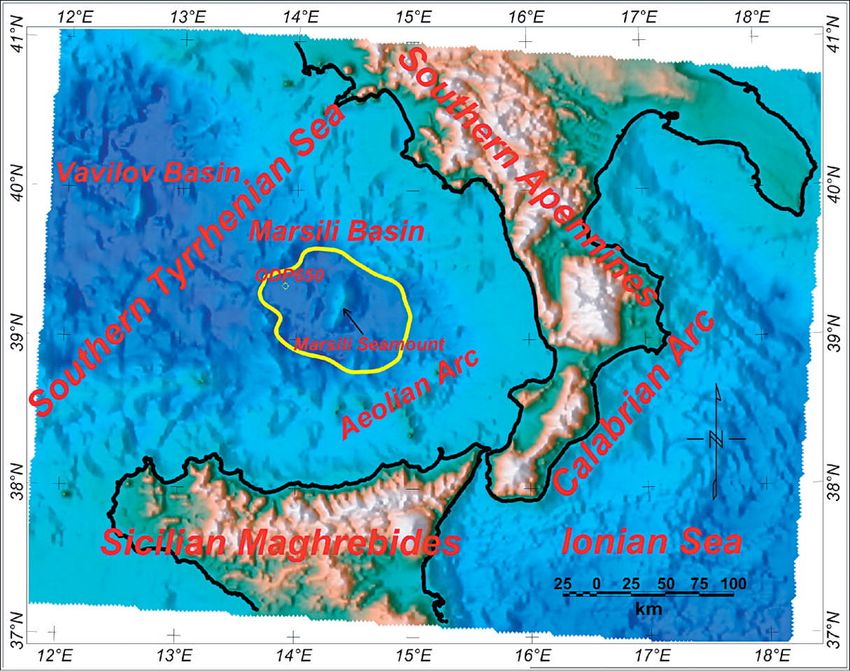
The anomaly field in Italy is characterized by a wide range of amplitudes and wave-
lengths and three major domains can be immediately seen at a first glance.

To the north, short-wavelength anomalies line up along the alpine belt, follow the arc
of the western Alps and continue southwards along the eastern coasts of Corsica
(the white, not surveyed island in the map). They mainly correspond to ophiolites
massifs, outcropping in the Alps and at shallow crustal depth below the Tyrrhenian
Sea to the East of Corsica.

South of latitude 41° N, the anomaly field on the Tyrrhenian Sea is characterized by
many anomalies of small extent, related to Pliocene and Pleistocene volcanic
edifices, comprising both seamounts and volcanic islands. On the contrary, the
Apennines mountain belt, all along the Italian peninsula, and the Adriatic Sea to the
east of it show a long-wavelength pattern. The different magnetic signature is mainly
due to the different types of crust: thin and with high heat flow below the Tyrrhenian
Sea, thick and with low heat flow below the eastern side of the Italian peninsula and
the Adriatic Sea.

These features entail an eastward dipping of the Curie
isotherm, as also suggested by the difference in the
anomalies’ background: a generally positive trend
characterizes the Adriatic region, whereas in the Tyrrhenian
Sea the short-wavelength anomalies stand out from a general
negative trend.
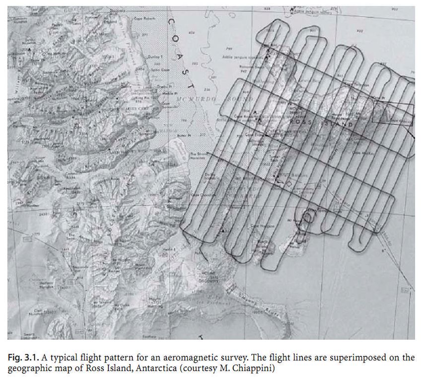
AEROMAGNETISM

An aeromagnetic survey is a survey of the Earth's magnetic field, based on data from
magnetometers towed behind aircraft or suspended below helicopters. These
instruments measure the total intensity of the geomagnetic field or,
occasionally, components of this field.

Resulting measurements can then be used to compute magnetic anomalies and can
be interpreted in terms of changes in the magnetic properties of the rocks below the
survey line or grid, the scale is from a few to hundreds of km..

The magnetometers are usually flown with other instrumentation, e.g. radiometric
and electromagnetic, at the lowest practicable constant height above the ground.
Usually the magnetometer is housed in a ‘bird’ towed behind the aircraft, or in a wing-
tip pod, or in a ‘stinger’ in the tail. When the magnetometer is on board, in-board coil
systems are used to compensate.
For mineral exploration

surveys generally have spacings in the range 50–200 m and are flown
perpendicular to the dominant geologic strike direction, although directions
no more than 45o from magnetic north are preferred because N-S
wavelengths are shorter than E-W wavelengths at low and intermediate
latitudes. For areas with distinct regions of differing geologic strike, costs
may permit splitting the survey into several flight directions or a single
compromise direction must be assigned.

hydrocarbon reservoirs are not directly detectable by aeromagnetic
surveys, but magnetic data can be used to locate geologic structures that
provide favorable conditions for oil/gas production and accumulation.
Similarly, mapping the magnetic signatures of faults and fractures within
water-bearing sedimentary rocks provides valuable constraints on the
geometry of aquifers and the framework of groundwater systems.
HELICOPTERS

Theoretical arguments suggest a line spacing to height ratio of 2 or less is
desirable to accurately sample variations in the magnetic field. The
majority of surveys, however, have ratios higher than this, i.e., 2.5 to 8.
Flight Altitude

For geologic mapping and mineral exploration surveys, measurements are
desirable at levels as close to the magnetic sources as possible, hence
surveys are flown at a constant height (mean terrain clearance) above the
ground surface. Prior to the availability of real-time global positioning system
(GPS) navigation, surveys over mountainous regions were flown at a constant
altitude.

This can improve the resolution of magnetic anomalies that is degraded by
flying at the higher constant altitude. However, current usage of more accurate
navigational systems (GPS) now permits fixed-wing surveys to be flown along
a preplanned artificial drape surface in regions of rugged topography. Post
survey processing of the collected magnetic field data could then be applied to
artificially “drape” the measurements onto a surface at some specified mean
terrain clearance.

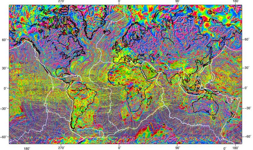
Publiclyavailable airborne
and marine magnetic data
have been
collected in North America
primarilyby the governments
of Canada,
the U.S., and Mexico. In the
early 1980’s, the fi rst
magnetic anomaly
map was produced for the
U.S. (Zietz, 1982). A digitized
version of
this analog map constitutes
most of the data for the
conterminous U.S.
in the North American
magnetic anomalymap
compilation (Com-
mittee for the Magnetic
AnomalyMap of North
America, 1987),
constructed as part of the
Geological Societyof
America’s Decade
of North American Geology
(DNAG) program. The
Canadian compo-
nent of the DNAG map was
based on a 2-km grid (Dods
and others,
DEPTH INTEGRATED MAGNETIC CONTRAST OVER USA
ORANGE /RED: HIGH SUSC CONTRAST
BLEU/LIGHT GREEN: LOW SUSC CONTRAST

Understanding the regional geology of the North American continent can provide
information useful for a wide variety of applications such as mineral and energy
resource assessments, earthquake and landslide hazards, and hydrologic and
environmental studies. Some applications of various high-resolution magnetic survey
(
A richness of geologic and
 tectonic detail at a range of
 scales can be seen.
 Southern Alaska has
 arcuate bands that parallel
 the modern volcanic arc.
 Northern Alaska has more
 subdued, generally
 equidimensional magnetic
 features. Central Alaska has
 a rich texture of short-
 wavelength features on a
 generally neutral magnetic
 background.

In Southern Alaska the arcuate, laterally continuous, deep magnetic features correlate spatially with the mapped
oceanic arc affinity terranes (as we would expect).
In Northern Alaska the general background of broad magnetic lows follow the thick sedimentary cover. The huge
North Slope magnetic high is enigmatic. The amplitude and wavelength of this deep magnetic high combined with the
lack of any suitable source rocks in the drilled portions of the sedimentary section, requires a deep, voluminous, and
highly magnetic source. It could represents mafic rocks in a failed continental rift, possibly of Devonian age.
Central Alaska has a generally average continental magnetic level punctuated by a series of relatively small and
discontinuous deep magnetic highs. These highs have a hit and miss correlation with mapped tectonic units; some of
the highs correlate with mapped Cretaceous and Tertiary igneous rocks.
The Portland-Vancouver survey
    was planned and the data were
    interpreted in cooperation with
    scientists from the Oregon
    Department of Geology and
    Mineral Industries and from
    Portland State University. These
    data are now being used by city,
    county, and state planners to
    assess the seismic hazard
    potential of the area.

The rainbow colors on this map represent "anomalies" of the magnetic field of the
earth over the Portland-Vancouver area. Reddish colors indicate anomalously strong
magnetic intensities, bluish colors relatively weaker intensities. The arrows highlight
the Portland Hills fault zone. The gray area in the inset map shows the most populated
areas of Portland and Vancouver.
Here a great deal of geological complexity is revealed reflecting repeated orogenesis (mountain building) and metamorphism since the time of the oldest known rocks, dating from the Archean. The patterns of repeated continental collisions and separations evident from more recent geology can be extrapolated into this past. However, poor rock exposure in most of the oldest, worndown areas of the world (Precambrian shields) hampers their geological exploration. Aeromagnetic surveys assist markedly here, though understanding at the scale of whole continents often necessitates maps extending across many national frontiers, as well as across oceans where present continents were formally juxtaposed.
LA CARTA AEROMAGNETICA D’ITALIA NELLA COMPILAZIONE DELL’AGIP

Negli anni ’70 poco prima del lavoro del PFG, per la ricerca di idrocarburi in
Italia, l’Agip ha realizzato dei rilievi aeromagnetici dell’intero territorio
nazionale e dei mari circostanti.

La Carta Magnetica, ossia la Carta delle anomalie del Campo Totale, venne
rappresentata con colori associati alle anomalie.

Dopo il segreto industriale negli anni 80’ l’AGIP aveva pubblicato una prima
versione della Carta che mostrava però evidenti indicazioni di un processing
non corretto dei dati raccolti.

Questa carta era inoltre notevolmente differente dalla carta al suolo del PFG
Versione iniziale (anni 80) Della carta
aeromagnetica delle Anomalie del
campo Magnetico totale in Italia
AGIP) e carta al suolo (INGV et al)

   Chiappini et al 2000
Different magnetic anomaly patterns

1) the Apennine mountain chain that acts as a rough sector of separation between the
   two Tyrrhenian and the Adriatic domains. On the Tyrrhenian side, anomalies start
   from a generally negative level while on the Adriatic basin a generally positive large-
   scale trend is present. This behaviour is not recognized at all on the aeromagnetic
   map.

2) The AGIP map showed a residual field with negative values on the Po Plain and
   strongly positive values over the Ionian Sea, with the isoanomaly lines almost
   orthogonal to the main Apennine compressive fronts, gradually increasing from the
   northern to the southern Apennines. The ground magnetic map shows a low
   amplitude positive anomaly along the whole external Apennine belt, adjacent to a
   negative residual field in the nearby Adriatic/Apulian foreland areas.

3) The NNW-SSE trending feature on the AGIP aeromagnetic map that has always
   been in disagreement with ground magnetic maps as well as with many other
   geophysical data and interpretations especially on the on shore areas, is now clearly
   defined.

   All these disagreements were likely due to an incorrect magnetic reference
   field removal undertaken on the aeromagnetic data set that, as reported by the
   same authors, was only based on the removal of a ‘magnetic field gradient’ for
   the whole covered area (see Cassano et al, 1986). This has dramatically
   produced a masking of low amplitude magnetic features.
A seguito di un dettagliato re-processing di tutti i dati è ora disponibile un
prodotto cartografico magnetico completamente nuovo. Il risultato finale
delle rielaborazioni è un database digitale organizzato sia per studi molto
dettagliati a carattere locale, sia per studi di grande scala, in dipendenza
dalle necessità dell’utente, mediante il quale Eni Exploration &
Production Division ha stampato una carta “shaded relief” in formato A0
in scala 1:1500000, con contour interval 10 nT, illuminata con
inclinazione 45° e declinazione 45°.

Qui di seguito viene riportata la nuova Carta Aeromagnetica d’Italia,
integrata e proiettata alla quota di riferimento di 2500 m. Ai singoli 36
rilievi acquisiti da Agip S.p.A.negli anni 1975-1979, sono stati rilevati ed
integrati 5 nuovi rilievi effettuati nel periodo 2001-2002 da Eni S.p.A.
Exploration & Production Division.

L’AGIP ha pubblicato anche (1986) una carta delle isobate del tetto del
cristallino e della sua suscettività magnetica.
Carta delle anomalie magnetiche del   Carta delle anomalie magnetiche del
campo totale in Italia al suolo       campo totale in Italia da aereo
Aeromagnetic map of Italy after new re-elaboration

Caratori Tontini et al. (2004)
30 years of magnetic investigations in Italy: tectonic
                 implications and perspectives
The first aeromagnetic map of Italy (Agip, 1981) did not show positive anomalies along the
Apennines: this was the premise for the thin-skinned models of the Apennines (Bally et al.,
Mostardini & Merlini, and many others….)

The aeromagnetic and ground level maps were reconcilied in 2004, when the aeromagnetic map
was revised using a more appropriate reference field. The two maps are now absolutely
consistent
The new magnetic maps from integration of measurements at ground and sea level did show a
positive anomaly of 10-30 nT (with some patches exceeding 100 nT) along the external belt: this
gave further support to thick-skinned tectonic models, which were in fashion then…

The revised Agip aeromagnetic map, more sensitive to deep sources, suggests that the positive
anomalies along the external Apennine belt and foreland are generated by the deep Adriatic crust,
before it deepens below the chain

Seismic data suggest that the lower crust of the northern Apennines (between 20 and 30 km depth,
likely yielding magnetic anomalies ) subducts along with underlying mantle beneath the belt.
Magnetic anomalies disappear where the lower crust subducts beneath the chain
Magnetic susceptibility of the lower crust may be in the order of 10-1 SI, thus 100-1000 times greater
than that of “crystalline basement”.

Additional geophysical proxies (and some work!!) are still needed to completely
interpret the magnetic fingerprint of the Apennines (and of orogens in general…)
Other examples…Geologic Hazard: the understanding of a volcano subsurface
Ultrafast oceanic spreading of the Marsili Basin, southern
  Tyrrhenian Sea: Evidence from magnetic anomaly analysis

Spectral analysis of both shipborne and airborne magnetic maps of the
southern Tyrrhenian Sea reveals seven subparallel positive-negative
magnetic anomaly stripes over the flat-lying deep floor of the Marsili
oceanic basin.
This represents the first evidence of oceanic magnetic anomalies in the
Tyrrhenian Sea. The central positive stripe is along the Marsili seamount, a
superinflated spreading ridge located at the basin axis. The stratigraphy of
Ocean Drilling Program Site 650 and K/Ar ages from the Marsili seamount
suggest that the Marsili Basin opened at the remarkable full-spreading rate
of ∼19 cm/ yr between ca. 1.6 and 2.1 Ma about the Olduvai subchron.
This is the highest spreading rate ever documented, including that
observed at the Cocos-Pacific plate boundary. Renewed but slow spreading
during the Brunhes chron (after 0.78 Ma), coupled with huge magmatic
inflation, gave rise to the Marsili volcano.
Our new data and interpretation show that backarc spreading of the
Tyrrhenian Sea was episodic, with sudden rapid pulses punctuating
relatively long periods of tectonic quiescence.
Figure 1. Digital elevation model (from National Geophysical Data Center ETOPO2 at
http://www.ngdc.noaa.gov/mgg/fliers/01mgg04.html) of southern Tyrrhenian Sea and
                                  surrounding areas.

       Nicolosi I et al. Geology 2006;34:717-720
Shipborne magnetic anomaly map of Marsili Basin and Magnetizations of 2A basalt layer
estimated from inversion of filtered anomalies
This represents the first evidence of oceanic magnetic anomalies in the
Tyrrhenian Sea. The central positive stripe is along the Marsili seamount,
Nicolosi I et al. Geology 2006;34:717-720 a superinflated spreading ridge located at the basin axis.Magnetic anomalies and crater impacts
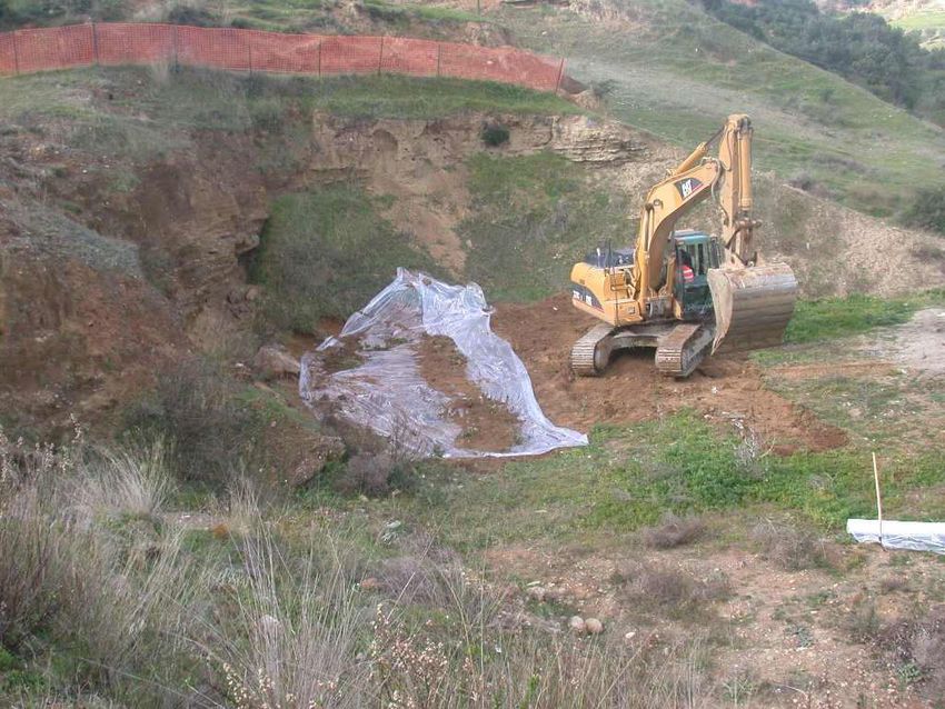
Indagini Ambientali con tecniche
magnetomeriche per l’individuazione di
corpi sepolti ad alta suscettività

Rilievi con magnetometri a pompaggio ottico
Il Supporto all’Archeologia
MAGNETIC SATELLITES I

L’importanza della conoscenza del campo da grande quota e’ evidente. Ad esempio anomalie
magnetiche con lunghezze d'onda di più di 500 km non sono determinabili semplicemente
ricucendo insieme rilievi effettuati in superficie. Solamente i satelliti possono offrire la prospettiva
globale. Brevi tempi di sorvolo, altitudine quasi costante sono altri benefici.

I satelliti OGO 2, 4 e 6 (POGO), inviati in orbita tra il 1965 ed il 1971, hanno condotto le prime di
misure di buona qualita’ utili ai fini della determinazione del campo magnetico principale e
crostale. il Magsat, il primo satellite nato appositamente per il geomagnetismo; con il Magsat si
sono misurati con buona precisione sia il valore del campo totale che quello delle sue componenti.
Lanciato nell'Ottobre 1979 questo satellite è rimasto in un'orbita solare sincrona fra i 352 e i 578
km di quota; dati sino al giugno 1980 quando il satellite è bruciato al rientro in bassa atmosfera.

Magsat ha contribuito notevolmente a far progredire le conoscenze sulla magnetizzazione della
litosfera mostrando che il debole campo magnetico litosferico è effettivamente discernibile alla
quota satellitare.

Purtroppo a causa di un livello elevato del rumore di fondo nelle misure e per l’orbita eccentrica, i
modelli di campo dedotti dai primi dati di satellite, non erano in buon accordo tra loro. Il livello
complessiva dell’intensita’ del campo litosferico differisce infatti tra i vari modelli di più di un fattore
2, corrispondendo ad un fattore 4 nella differenza tra gli spettri di potenza.

Specificamente per quanto riguarda la conoscenza del contributo crostale al magnetismo dopo
questi successi iniziali per circa un ventennio non si erano avuti nuovi dati da satellite.
Recentemente invece nuovi satelliti appositamente progettati per misure magnetiche forniscono
nuovi dati
MORE RECENT MAGNETIC SATELLITES

ØRSTED Altitude: 620 to 850 km, elliptic Inclination: 96.62
degrees, approximately polar, Magnetic instrumentation: 8
m boom w. triaxial compact spherical coil fluxgate and
scalar Overhauser magnetometer (0.1 nT). Orientation:
non-magnetic star camera. Launched 1999.

CHAMP nearly circular, polar orbit with an initial altitude of
455 km, decaying to 300 km over a life span of 5 years;
eccentricity about 0.001. Magnetic instrumentation: 4 m
boom w. triaxial fluxgate, Overhauser scalar (0.1 nT).
launched in July 2000
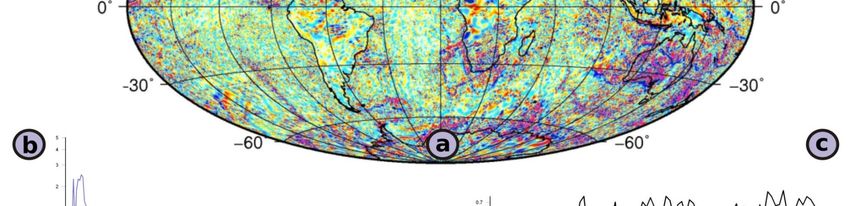
The resulting total
intensity anomaly
from CHAMP map
provide a new basis
for studies of crustal
structure, dynamics
and heat flow.

The map gives an
improved account
of the long crustal
wavelengths, as is
apparent in the
Atlantic Ocean
and in the Arctic,
where structures
are well aligned
with the Mid
Ocean Ridge.
A) The contrast between a weakly magnetized oceanic and a strongly
   magnetized continental lithosphere, scaling with the strength of the main
   field in a non-trivial way.

B) the magnetization in the Pacific turns out to be even weaker than previously
    assumed, with some notable exceptions in the west.

C) Surprisingly, anomaly amplitudes over the Arctic Ocean are higher than over
   Antarctica. Magsat and Ørsted have gaps of 7º in radius at the poles, which
   raised questions about the reliability of the earlier field models in the polar
   caps. It is therefore remarkable that a large positive anomaly in the
   American sector of the Arctic Ocean close to the North Pole, present in
   ALP94, CWKS89 and CM3, has now been confirmed by CHAMP with its
   polar gap of only 2.7º.

D) On the other hand, large Antarctic anomalies given by CM3 and CWKS89
   have not been confirmed. They may be due to auroral ionospheric currents
   because the Magsat mission was confined to the Antarctic summer.
   compilations
Verso una visione globale delle anomalie planetarie
Magnetic Anomaly Map of the World (Mercator). The anomaly field is shown at an altitude of 5 kilometers
above the WGS84 ellipsoid. The near-surface compilations are distinguished from the satellite-based and
oceanic model data by way of shading, and their distribution can be seen in the index map included within
the map. Finally, the entire data set is displayed using the natural color scale (red = high, blue = low) with a
shaded relief effect using artificial illumination. The white lines on the map locate undifferentiated tectonic
elements and include ridges, fracture zones, and trenches. The original map is at a scale of 1:50 million.
Magnetic Anomaly Map of the World (Mercator). The anomaly field is shown
at an altitude of 5 kilometers above the WGS84 ellipsoid. The near-surface
compilations are distinguished from the satellite-based and oceanic model
data by way of shading, and their distribution can be seen in the index map
included within the map. Finally, the entire data set is displayed using the
natural color scale (red = high, blue = low) with a shaded relief effect using
artificial illumination. The white lines on the map locate undifferentiated
tectonic elements and include ridges, fracture zones, and trenches. The
original map is at a scale of 1:50 million.
Planetary Magnetic Fields

     Many spacecraft carry Magnetometers to measure the Magnetic Field

Mars Global Surveyor    Advanced Composition Explorer          Galileo
Distan Radius Mass Rotatio # Orbital Orbital Obliqu Orbita Densit
ce (Earth' (Earth' n Moon Inclinat Eccentri ity l y
(AU) s) s) (Earth' s ion city period (g/cm3
s) )
Sun 0 109 332,80 25-36* 9? --- --- --- 1.410
Mercury 0.39 0.38 0.05 58.8 0 7 0.2056 0.1° 0,241 5.43
Venus 0.72 0.95 0.89 244 0 3.394 0.0068 177.4° 0,615 5.25
Earth 1.0 1.00 1.00 1.00 1 0.000 0.0167 23.45° 1 5.52
Mars 1.5 0.53 0.11 1.029 2 1.850 0.0934 25.19° 1.881 3.95
Jupiter 5.2 11 318 0.411 (63) 1.308 0.0483 3.12° 11.87 1.33
Saturn 9.5 9 95 0.428 (62) 2.488 0.0560 26.73° 29.45 0.69
Uranus 19.2 4 17 0.748 (27) 0.774 0.0461 97.86° 84.07 1.29
Neptune 30.1 4 17 0.802 (13) 1.774 0.0097 29.56° 164.9 1.64
Pluto 39.5 0.18 0.002 0.267 (3) 17.15 0.2482 119.6° 248.1 2.03Other Planets in our Solar System have Magnetic Fields
Mercury

               Mercury has a weak magnetic field.

             This suggests Mercury has an iron core
                       with liquid interior.

              The weak magnetic field could be the
                result of the slow rotation period.

Venus
          Venus has a very weak magnetic field.(About
              100,000 times weaker than Earth’s)

               Venus appears to lack the necessary
             ingredients to generate a magnetic field
                        (no liquid core ?)

                Venus also has very slow rotation.
Mars Mars also has a very weak magnetic field.
(About 5,000 times weaker than Earth’s)
The interior of Mars appears to have cooled
so much that it is no longer liquid.
• The volcanoes in Mars are no longer active
• There is no Earthquake activity on MarsJupiter Jupiter has a strong magnetic field.(About 20,000
times stronger than Earth’s)
The Terrestrial planets generate magnetic fields
from iron at the center.
But Jupiter has almost no iron core.
The magnetic field of Jupiter is produced by the
motion of liquefied metallic hydrogen found
beneath the surface.
Saturn
Saturn also has a strong magnetic field.
(About 540 times stronger than Earth’s)
Saturn’s magnetic field is produced in the
same way Jupiter’s is.Uranus
The magnetic field in Uranus is about 40 times
stronger than Earth’s
It is probably created in the core of the planet,
with ice, rather than with iron.
Neptune
The magnetic field in Neptune is about 1/4
times as strong as Earth’s
It is probably created in the same way as Uranus
No news from Pluto…Because Pluto has a small size and a
slow rotation rate (1 day in Pluto = 6.4 Earth days), it does not
seem likely that Pluto has a magnetic field.Planet Earth Jupiter Saturn Uranus Neptune Radius, km 6,378 71,400> 60,300 25,600 24,800 Spin period, hrs 24 9.9 10,7 17.2 16 Magnetic Moment/MEarth 1 20,000 600 50 25 Mean equatorial field, gauss 0.31 4.28 0.22 0.23 0.14 Dipole tilt and sense +11.3° -9.6° 0° -59° -47° Solar Wind density, cm-3 10 0.4 0.1 0.03 0.005 Distance to "nose", planet. radii 11 50-100 16-22 18 23-26
You can also read