MARS 2020 SHERLOC PDS Archive User's Guide - Mars 2020 SHERLOC Archive User's Guide
←
→
Page content transcription
If your browser does not render page correctly, please read the page content below
Mars 2020 SHERLOC Archive User’s Guide                                               July 21, 2021

                MARS 2020
       SHERLOC PDS Archive User’s Guide

                                            Version 0.3

                                           July 21, 2021

Prepared by: Kyle Uckert - Jet Propulsion Laboratory, California Institute of Technology

Custodian: Kyle Uckert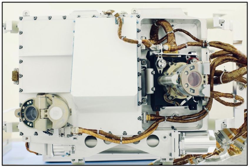
Mars 2020 SHERLOC Archive User’s Guide                                                                                         July 21, 2021

1.     Overview ................................................................................................................................. 3
     1.1.     What is SHERLOC?........................................................................................................... 3
     1.2.     SHERLOC Operations....................................................................................................... 3
     1.3.     Typical SHERLOC Activities .............................................................................................. 5
     1.4.     SHERLOC Data Products .................................................................................................. 6
     1.5.     The SHERLOC Archive Bundle ......................................................................................... 8
2.     Documents ............................................................................................................................ 10
3.     Raw Products ........................................................................................................................ 11
     3.1.     Raw Spectral Products .................................................................................................. 11
     3.2.     Raw Image Products ..................................................................................................... 12
4.     Derived Products................................................................................................................... 12
     4.1.     Derived Spectral Products ............................................................................................ 12
     4.2.     Derived Imaging Products ............................................................................................. 13
5.     Calibration Products ............................................................................................................. 14
6.     Data Collection and Caveats ................................................................................................. 15
     6.1.     Data Acquisition and the SHERLOC DUV Laser ............................................................. 15
     6.2.     Data Processing ............................................................................................................. 15
     6.3.     Processing Not Included in this Pipeline ....................................................................... 16
7.     Acknowledgements: ............................................................................................................. 16
Appendix A: ................................................................................................................................... 17
Appendix B .................................................................................................................................... 21

© 2021. California Institute of Technology. Government sponsorship acknowledged.                                                                 2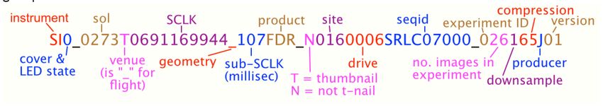
Mars 2020 SHERLOC Archive User’s Guide                                             July 21, 2021

1. Overview
This document is a quick start guide to the Mars 2020 SHERLOC data archive. This document is
intended to give users a basic understanding of the SHERLOC archive, where to find relevant
data products and information, and identify any caveats on data collection.

   1.1. What is SHERLOC?
SHERLOC (Scanning Habitable Environments with Raman and Luminescence for Organics and
Chemicals) is a robotic arm-mounted instrument on NASA’s Perseverance rover. SHERLOC has
two primary boresights. The Spectroscopy boresight generates spatially resolved chemical maps
using fluorescence and Raman spectroscopy coupled to microscopic images (10.1 µm/pixel).
The second boresight is the Wide Angle Topographic Sensor for Operations and eNgineering
(WATSON); a copy of the Mars Science Laboratory (MSL) Mars Hand Lens Imager (MAHLI) that
obtains color images from microscopic scales (~13 µm/pixel) to infinity. SHERLOC Spectroscopy
focuses a 40 µs pulsed deep UV neon-copper laser (248.6 nm), to a ~100 µm spot on a target at
a working distance of ~48 mm. Fluorescence emissions from organics, and Raman scattered
photons from organics and minerals, are spectrally resolved with a single diffractive grating
spectrograph with a spectral range of ~250 to ~354 nm. Because the fluorescence and Raman
regions are naturally separated with deep UV excitation (
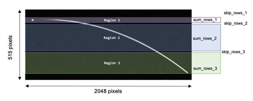
Mars 2020 SHERLOC Archive User’s Guide                                                                          July 21, 2021

Figure 1: A photograph of the SHERLOC turret assembly before integration with the rover robotic arm. The right boresight is the
WATSON color imager, and the left boresight is the ACI imager and spectrometer. The dust cover is open for the spectroscopy
boresight in this image.

When in focus, the objective lens focuses the laser to a 100-110 µm diameter spot. Incident
DUV laser pulses are focused on a target, using the moveable scanner mirror to sweep over an
area to generate a map. The Raman and fluorescence photons excited by the laser are collected
by the common-path ACI objective lens. The Raman scattered and fluoresced light is focused
across the long axis of the 512-by-2048 pixel Spectrometer CCD (SCCD). The off-axis nature of
the spectrometer’s optical design causes a physical curving of the spectrum across the SCCD
focal plane, which is referred to as a spectral smile, shown in Figure 2.

Figure 2: Illustration of the SCCD detector array overlayed with the spectrometer "smile" pattern and the on-chip integration
patterns.

© 2021. California Institute of Technology. Government sponsorship acknowledged.                                                4
Mars 2020 SHERLOC Archive User’s Guide                                                July 21, 2021

Data is read out in a columnar fashion, typically using three binned regions, as shown in Figure
1: Region 1 collects the Raman signal from 250 to 282 nm (225 to 4760 cm-1), while Regions 2
and 3 collect fluorescence up to 355 nm. Dividing the SCCD into multiple regions minimizes
noise and allows for configurable clock speeds and variable gain settings. These variable gain
settings provide the flexibility to change the electrons/count for a binned region to
accommodate the dynamic range necessary to acquire both low Raman signals, and the
relatively more intense fluorescence signals, which may saturate the detector if a single gain
setting were applied across the entire SCCD.
Each time a SHERLOC spectrum is collected, two frames are acquired: an active frame (with the
laser firing at the target) and a dark/background frame (of the same duration as the active
frame, but without the laser firing). The dark frame may be subtracted from the active frame to
remove pixel-to-pixel variability in the SCCD.
The first and last 50 pixels on the SCCD are not light sensitive and do not contain spectral data.
The intensity values for these channels are reported in the EDR and RDR products described
below, and may be used for dark noise characterization. Typically, an end user would ignore
these channels when generating a spectrum.
During spectroscopy map measurement collection, the laser intensity may decrease over time
as the temperature increases due to use. The laser photodiode tracks the laser output, and may
be used to normalize all spectra within a map to provide direct comparisons between spectral
measurements.

   1.3. Typical SHERLOC Activities
A typical SHERLOC mapping sequence runs through the following elements in order, described
in detail below. Note, SHERLOC sequences may deviate from this typical plan to include
additional ACI imaging and additional spectral map acquisitions observations following Process
Data algorithm execution.
   •   Internal AlGaN calibration target measurement
   •   ACI image focus stack (subframes)
   •   ACI image focus
   •   SHERLOC spectroscopy map acquisition
   •   Process Data algorithm execution
   •   ACI image focus stack (subframes)
   •   ACI image focus
   •   Internal AlGaN calibration target measurement
A SHERLOC activity begins by using the Autofocus Context Imager (ACI) to obtain target focus
and to acquire a 10.1 µm/pixel greyscale image. The ACI focus mechanism is stepped through a
range of motor positions, with the ideal focus position determined by calculating the maximum
compression ratio of all images acquired in the stack. A full frame ACI image is acquired at the
best focus position, and the focus mechanism is offset ~150 µm to focus the spectrometer.

© 2021. California Institute of Technology. Government sponsorship acknowledged.                     5
Mars 2020 SHERLOC Archive User’s Guide                                              July 21, 2021

SHERLOC acquires a spectral map at the focus position with a defined map size, spacing, and
number of laser shots per point. SHERLOC is not restricted to using pre-defined scanner tables,
and may generate maps with irregularly spaced points. Default maps typically selected for
reconnaissance of a target will generally include 7x7 mm survey mode scans (36 x 36 point grid
or 10 x 10 point grid) and detailed-mode scans (5x5 mm or 1x1 mm grids with up to 1296
points) for follow-up measurements of regions of interest (ROIs). These ROIs may be selected
autonomously by the on-board SHERLOC Process Data algorithm.
After the SHERLOC spectroscopy measurements have been collected, the data may be
processed using on-board algorithms (called Process Data mode). This processed data will have
a lower data volume, and may be downlinked for tactical decision-making before the full
spectral map is available. On-board Process Data algorithms consist of:
   [0] Copy Raw
   [1] Background Subtraction: subtracting the dark frames from the active frames
   [2] Laser Normalization: normalize all spectra to account for laser energy variability, as
        measured by the laser photodiode
   [3] Raw Photodiode Dump: the returned data product includes all photodiode
        measurements
   [4] Summary Photodiode Dump: the returned data product includes the average
        photodiode value for each map point
   [5] Hot Pixel Removal
   [6] Cosmic Ray Removal: (see Document [14] for details)
   [7] Zone Specification: selection of up to six spectral ranges
   [8] Spectral Binning: sum spectral channels in specified spectral zones
   [9] Spatial Binning: sum spectral intensity values for all channels within pre-defined spatial
        regions of a default map
   [10] Ranking: rank each spectrum based on the spectral zones, zone weights, and spectral
        intensity within each zone. Spatial locations with high ranking may be selected for
        autonomous follow-up detailed-mode spectral measurements.
After spectral acquisition and Process Data algorithms are applied, focused ACI subframe and
full frame images are acquired. The initial and final ACI images and their focus positions may be
used to characterize any robotic arm drift that may have occurred during the measurement.
Additional images may be commanded during spectroscopy acquisition to provide finer
resolution drift characterization, if necessary.

   1.4. SHERLOC Data Products
The SHERLOC ground processing tools generate two types of data products that are archived in
the PDS:
   •   EDRs (Engineering Data Records) – raw, un-calibrated data products
   •   RDRs (Reduced Data Records) – calibrated and/or processed data products. RDR
       products are generally the products a SHERLOC data user will use for analysis of a
       target.

© 2021. California Institute of Technology. Government sponsorship acknowledged.                6
Mars 2020 SHERLOC Archive User’s Guide July 21, 2021
Each of the SHERLOC EDR and RDR products are described in detail in the EDR/RDR SIS
(Documents [6] and [7]) and summarized below in Section 3 and 4.
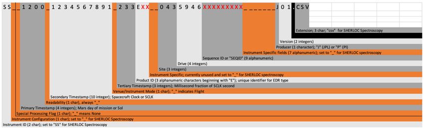
The SHERLOC data products follow the M2020 filename convention:
See Appendix A for a detailed description of each of these filename fields.
Filename Prefix:
• SS: SHERLOC Spectroscopy
• SC: SHERLOC Context Imager (ACI)
• SI: SHERLOC Imaging (WATSON)
• SE: SHERLOC Engineering (state-of-health information)
Product ID:
Values Description
EDF Engineering data in fault detection (cruise phase data only)
EDR Science data frame (cruise phase data only)
ESH Spectroscopy state of health in science mode
ECH Spectroscopy state of health in calibration mode
EXH Scanner position array (in pixel)
ERA Full resolution active spectra in science mode
ERB Full resolution background (dark) spectra in science mode
ECA Full resolution active spectra in calibration mode
ECB Full resolution background (dark) spectra in calibration mode
EPA Photodiode array
ESP Scanner position array (in millimeter unit of measurement)
RRA Active frame, with or without processing (see instrument-specific filename field) in science
mode
RRB Dark frame, with or without processing (see instrument-specific filename field) in science
mode
© 2021. California Institute of Technology. Government sponsorship acknowledged. 7Mars 2020 SHERLOC Archive User’s Guide July 21, 2021
RCA Active frame, with or without processing (see instrument-specific filename field) in
calibration mode
RCB Dark frame, with or without processing (see instrument-specific filename field) in calibration
mode
RRS Dark-subtracted spectrum – see instrument-specific field for processing applied in science
mode
RCS Dark-subtracted spectrum – see instrument-specific field for processing applied in
calibration mode
RCC Internal AlGaN peak assessment summary, used to determine spectral alignment
RLP Scanner position table in scanner azimuth/elevation and target (mm) space
RLS Laser shot positions for each ACI image
RLI Laser intensity map
RM* Spectral intensity map for pre-defined spectral ranges
RMO Spectral intensity map and laser shot position summary
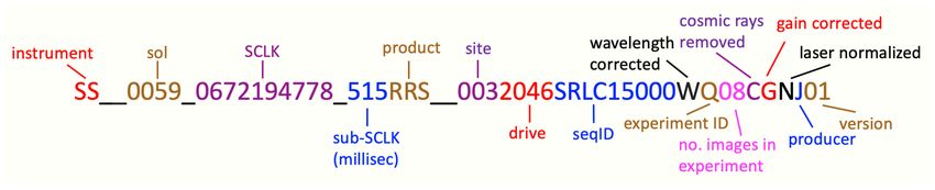
The instrument-specific field of the filename includes information on the processing performed
and on linking the imaging and spectroscopy data files together. The SS* files use seven
characters for this field, and SC* and SI* files use four characters. See the table above for an
overview of valid values and the associated processing performed.
Example filenames:
The example below shows a SHERLOC imaging file name, along with descriptions of character
groups.
The example below shows a SHERLOC spectroscopy file name, along with descriptions of
character groups.
1.5. The SHERLOC Archive Bundle
The data acquired by SHERLOC is archived in the PDS within the mars2020_sherloc bundle. The
bundle contains collections of SHERLOC products based on data processing level and type. Within
data collections, products are sorted into subdirectories by Sol number. Products in the sub-
directories are identified by the three-letter code found in positions 24-26 of the file name.
© 2021. California Institute of Technology. Government sponsorship acknowledged. 8Mars 2020 SHERLOC Archive User’s Guide July 21, 2021
The structure of the mars2020_sherloc bundle is:
mars2020_pixl
data_raw_spectroscopy
sol_xxx
ECH, ESH – Spectroscopy state of health
ECA, ECB – Active and dark frame calibration spectra
ERA, ERB – Active and dark frame science spectra
ERP – Process_Data spectra
ESP – Scanner position
EPA – Laser photodiode
data_aci_imgops
sol_xxx
EDR – context image
ECM – companded images
ECZ, EZS – Z-stack images
EDM – focus merge image
data_watson_imgops
sol_xxx
EDR – context image
ECM – companded images
ECZ, EZS – Z-stack images
EDM – focus merge image
data_spectroscopy
sol_xxx
RCA, RCB – processed active and dark spectra (calibration target)
RRA, RRB – processed active and dark spectra (science target)
RCS – dark-subtracted spectra (calibration target)
RRS – dark- subtracted spectra (science target)
RAC, RBC, RAR, RBR – cosmic ray candidate lists
RCC – internal AlGaN calibration target fit results
RLS – laser shot position tables
RMO – laser shot and spectral position tables
RMx – selected integrated intensity maps
data_aci
sol_xxx
RAD – Radiometrically-corrected image
data_watson
© 2021. California Institute of Technology. Government sponsorship acknowledged. 9Mars 2020 SHERLOC Archive User’s Guide July 21, 2021
sol_xxx
RAD – Radiometrically-corrected image
Document
SHERLOC EDR SIS
SHERLOC RDR SIS
SHERLOC Bundle SIS
2. Documents
These publications or websites describe the Planetary Data System Standards used to produce
the SHERLOC archive. These documents are archived in the PDS system and are not found
specifically in the SHERLOC archive. These documents are revised approximately every six
months with each new release of the PDS Information Model. Current and previous versions
may be found at the links below.
[1] PDS4 Concepts Document, https://pds.nasa.gov/datastandards/documents/concepts/.
[2] Planetary Data System Standards Reference,
https://pds.nasa.gov/datastandards/documents/sr/.
[3] Planetary Data System Data Provider’s Handbook,
https://pds.nasa.gov/datastandards/documents/dph/.
[4] PDS4 Common Data Dictionary, Abridged,
https://pds.nasa.gov/datastandards/documents/dd/.
[5] PDS4 Information Model Specification,
https://pds.nasa.gov/datastandards/documents/im/.
These documents describe the specifics of the archive and the archive data products, and can
be found in the SHERLOC document collection (i.e. mars2020_SHERLOC:document).
[6]
[7]
[8]
[9]
These papers describe in detail the Mars 2020 mission and the SHERLOC instrument. These
papers are published with open access and can be downloaded by following the DOI.
[10] Farley, K.A., et al. (2020), Mars 2020 Mission Overview, Space Sci. Rev. 216:142,
doi:10.1007/s11214-020-00762-y.
[11] R. Bhartia, L.W. Beegle, L. DeFlores, et al. “Perseverance’s Scanning Habitable
Environments with Raman and Luminescence for Organics and Chemicals (SHERLOC)
Investigation”. Space Sci. Rev. 2021. paper in press.
© 2021. California Institute of Technology. Government sponsorship acknowledged. 10Mars 2020 SHERLOC Archive User’s Guide July 21, 2021
[12] Uckert, K., Bhartia, R., Beegle, L. et al. (2021) “Calibration of the SHERLOC Deep UV
Fluorescence/Raman Spectrometer on the Perseverance Rover”. Applied
Spectroscopy, accepted.
[13] Razzell Hollis, J., Abbey, W., Beegle, L., et al. (2021) “A Deep-Ultraviolet Raman and
Fluorescence Spectral Library of 62 Minerals for the SHERLOC instrument onboard
Mars 2020”. Submitted to Planetary and Space Sciences.
[14] Uckert, K., Bhartia, R., Michel, J. "A semi-autonomous method to detect cosmic rays in
Raman hyperspectral data sets." Applied spectroscopy 73.9 (2019): 1019-1027.
3. Raw Products
3.1. Raw Spectral Products
All EDR products contain several tables with instrument state-of-health (SOH) data,
followed by spectral, laser photodiode, or scanner position data tables.
SOH data tables:
State of health data tables include data used by the SHERLOC operations team to evaluate
the health of the instrument, and includes: temperatures for each SHERLOC subsystem,
arguments used to command the instrument, SCCD configuration parameters, scanner
configuration parameters, command timing information, instrument status flags (indicating
the state of each subsystem at a specified time), and laser configuration parameters. See
Document [7] for a full description of each table entry. This information may not be useful
for an average science data product user.
ERA/ERB/ERS/ECA/ECB:
These products contain the raw spectral data for the active or dark frame, or dark-
subtracted spectra, in the case of background-subtracted process data spectral products
(ERS). Spectra from each region are listed, starting with a single line table header (e.g.
DARK_SPECTRA_REGION_1:), followed by column headers (e.g. R1_Channel_0). All spectral
information are listed in data tables of size N x 2148 x R, where N is the number of spectra
(represented as a row in each table), 2148 represents the number of wavelength elements
(represented by columns in each table), R represents the number of regions (represented
by tables in the csv file – usually 3 regions are implemented).
EPA:
The laser photodiode data is listed in a table following the SOH entries. The table identifier
(e.g. LASER_PHOTODIODE_DATA) precedes the table column headers (e.g. shot_number_0).
The laser photodiode table is of size N x S, where N is the number of spectra (represented
as a row in the table) and S is the number of shots in each spectrum (represented as
columns in the table).
© 2021. California Institute of Technology. Government sponsorship acknowledged. 11Mars 2020 SHERLOC Archive User’s Guide July 21, 2021 ESP: The scanner data is listed in a table following the SOH entries. The scanner position data associated with the spectra is stored in a table of size N x 2, where N is the number of spectra (represented as a row in the table) and 2 is the number of position elements – azimuth and elevation (represented as columns in the table). If the LOAD_TABLE command is issued, a second table containing the commanded azimuth and elevation values will be present as a second table. The measured scanner position errors and scanner current tables are the last tables in the file. 3.2. Raw Image Products ECM: Contains companded data either as originally downlinked or JPEG decompressed. ECZ: A best-focus Z-stack image, created onboard the instrument from a combination of images at different focus settings, with a much greater depth of field. EDM: Second of two products produced by onboard focus merge (z-stacking). This single-band grayscale image provides information about which images the best-focus data came from, and can provide a crude measure of target surface relief. DN of 255 indicates first image in the Z-stack, while the last is dependent on number of image-merge, with linear scaling between. EDR: Nominal data product. EZS: A best-focus Z-stack image, created on the ground from a combination of images at different focus settings, with a much greater depth of field. 4. Derived Products 4.1. Derived Spectral Products RDR products do not contain the instrument state-of-health (SOH) data table present in the EDRs, but follow the same general format for spectral data. It is anticipated that the primary data products needed by a SHERLOC data user will be the RRS (dark-subtracted spectra) and the RLS (laser shot position table) RDRs. RRA/RRB/RRS: © 2021. California Institute of Technology. Government sponsorship acknowledged. 12
Mars 2020 SHERLOC Archive User’s Guide                                              July 21, 2021

   The RRA and RRB products contain spectral products that have been processed in some
   way, which may include cosmic ray correction, gain correction, wavelength correction,
   and/or laser normalization. The instrument-specific field of the filename indicates the kind
   of processing that has been applied (see Appendix A). RRS products contain dark-subtracted
   spectra, and may also include aforementioned processing. If wavelength calibration has
   been performed, the first table will include wavelength (nm) assignments for each SCCD
   channel.

   RCC:
   This product contains a summary of the spectral alignment of SHERLOC based on fits to
   peaks in measurements of the internal AlGaN target.

   RM*:
   The integrated intensity within a specified wavelength region for each point is calculated
   and reported in a table with a single column. The wavelength regions are selected by the
   SHERLOC team, and may be used to automatically generate maps for Autolook and
   Quicklook product generation, however future science users may find it more convenient to
   generate their own maps from RRS product data.

   Up to 35 RM* products may be generated for each RDR data set, with the first 6 reported in
   the Autolook report.

   RLI:
   This product contains the laser intensity map table – a single column with the average
   photodiode data. This product is used by the SHERLOC team during operations to map the
   laser power output.

   RLS:
   This product contains a table with all laser shot positions mapped to pixel positions in each
   ACI image.

   RMO:
   This product contains a summary of laser shot positions (present in the RLS product), and
   the spectral intensity maps (present in the RM* products), along with the wavelengths used
   for each spectral intensity map. The RMO product may be used to generate a multispectral
   image of the target with the pre-selected wavelength ranges, which may be useful for
   generating Quicklook products and rapid assessment for tactical decision-making.

   4.2. Derived Imaging Products
   RAD:
   Radiometrically-corrected images. Radiometric correction is the process of converting the
   image to a calibrated unit that represents the light entering the lens of the camera. It thus

© 2021. California Institute of Technology. Government sponsorship acknowledged.               13
Mars 2020 SHERLOC Archive User’s Guide July 21, 2021
provides a representation of the scene as it exists, independent of the camera. It should
not be confused with photometric correction, which takes into account lighting and
geometry in order to describe the objects in the scene, independent of how they were
observed. As of this version of the SHERLOC User’s Guide, a radiometric model for the
SHERLOC cameras is not well-calibrated, and RAD products should not be considered in
data analysis.
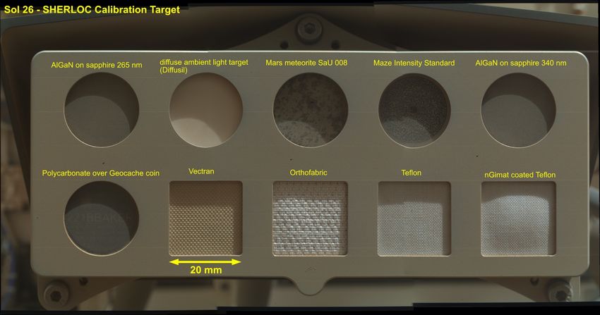
5. Calibration Products
SHERLOC includes 11 calibration targets. Products associated with the internal AlGaN target are
denoted with special EDR and RDR product IDs (ECA, ECB, RCA, RCB, RCS). External calibration
targets will have Sequence ID fields that start with SRLC15*, with the external calibration target
indicated in the LBL file under the CAL_TARGET_NAME field.
• An internal AlGaN target, with a central peak at ~277 nm. This target is measured after
SHERLOC powers on to collect measurements and right before SHERLOC powers off.
• An external calibration palette, which will be measured less frequently, and includes the
following targets:
o 1) AlGaN on Sapphire (peak wavelength at 262.5 nm)
o 2) Diffusil Diffuser
o 3) Mars Meteorite SaU 008
o 4) Intensity Target (maze, chrome on fused silica glass)
o 5) AlGaN on Sapphire (peak wavelength at 335 nm)
o 6) Polycarbonate visor material over Geocache opal glass
o 7) Vectran spacesuit material
o 8) Orthofabric spacesuit material
o 9) Teflon spacesuit material
o 10) nGimat-coated Teflon spacesuit material
© 2021. California Institute of Technology. Government sponsorship acknowledged. 14Mars 2020 SHERLOC Archive User’s Guide July 21, 2021 6. Data Collection and Caveats 6.1. Data Acquisition and the SHERLOC DUV Laser The SHERLOC laser configuration parameters should be noted when comparing SHERLOC datasets. The number of pulses per point, the laser rep rate, laser current, and the SCCD temperature may all be retrieved from the EDR SOH tables. The SCCD temperature is kept constant during a SHERLOC measurement through the use of a phase-change material, described in Document [2], however, operations outside of ideal times may cause some thermal variability to be observed during a measurement, which is usually in the order of 15 minutes for the largest maps. Inherent to NeCu deep UV lasers are multiple laser lines that can be generated at different output energy levels. While most of these lines have been removed by SHERLOC’s laser- conditioning optics, a small fraction of the 252.93 nm line reflected from a target may be observed at an intensity comparable with a strong Raman band. This line may obscure Raman features that coincide with this region of the spectrum (650 – 750 cm-1). 6.2. Data Processing The SHERLOC processing pipeline automatically removes cosmic ray noise spikes from spectra using the algorithm described in Document [14]. This algorithm is somewhat dependent on the tunable input parameters, including the threshold multiplier and the sigma clipping coefficient, which may be changed to improve performance. At the start of the mission, these parameters may not be fine-tuned, and many cosmic rays may still be present in the resulting RRA, RRB, and RRS RDR products. © 2021. California Institute of Technology. Government sponsorship acknowledged. 15
Mars 2020 SHERLOC Archive User’s Guide                                              July 21, 2021

   The laser photodiode can be used to monitor the laser output energy level within a map,
   but should not be used to compare laser output energy for spectra collected on different
   Sols, or on different materials. The laser photodiode intensity may increase when measuring
   highly reflective targets (as is observed on the maze intensity calibration target), and has
   been observed to slightly depend on the optical bench temperature.

   6.3. Processing Not Included in this Pipeline
   RDRs generated as part of the SHERLOC PDS archive will not include baseline subtraction
   (which may be used to correct for variable fluorescence intensity) or Raman peak fitting.
   This processing usually requires a human-in-the-loop to be effectively implemented, and
   commercial and open-source tools exist to complete this processing, if desired. Document
   [13] contains an overview of baseline subtraction applied to SHERLOC data, and Document
   [14] contains information on fitting Raman peaks in SHERLOC data.

7. Acknowledgements:
 The research was carried out at the Jet Propulsion Laboratory, California Institute of
Technology, under a contract with the National Aeronautics and Space Administration
(80NM0018D0004)

© 2021. California Institute of Technology. Government sponsorship acknowledged.              16
Mars 2020 SHERLOC Archive User’s Guide                                                         July 21, 2021

Appendix A:
 Characters   Contents                        Description
 1-2          Instrument                      SS: SHERLOC Spectroscopy
                                              SC: SHERLOC ACI
                                              SI: SHERLOC WATSON
 3            Configuration                   “_” for SHERLOC spectroscopy and engineering
                                              For image products, cover and LED state:
                                               0         Cover closed, LEDs off
                                               1         Cover open, LEDs off
                                               2         Cover closed, LEDs on
                                               4         Cover closed, LEDs on
 4            Special Processing Flag         “_” (none for SHERLOC)
 5-8          Sol                             Sol number for flight surface data; see EDR SIS for other
                                              uses
 9            Mission venue                   “_” for Flight Mode
 10-19        Spacecraft Clock Count (SCLK)   10-integer spacecraft clock count in seconds
 20           Underscore                      Always “_” for readability
 21-23        Fractional SCLK                 3-digit spacecraft clock count fractional seconds
 24-26        Product Type                    See SHERLOC Product Type in Table 1

 27           Geometry                        Not used for Spectroscopy, set to “_”.

                                              For image products: denote for Geometry for WATSON and
                                              ACI:
                                              “_” indicates raw (non-linearized) geometry
                                              “L” indicates product has been linearized with nominal
                                              stereo partner
                                              “A” indicates product has been linearized with actual stereo
                                              partner

 28           Thumbnail                       “_” for non-image products
                                              “T”: Product is a thumbnail images
                                              “N”: Product is not a thumbnail image
 29-31        Site                            Site identifier from Rover Motion Counter
 32-35        Drive                           Drive identifier (position within a site location)

© 2021. California Institute of Technology. Government sponsorship acknowledged.                          17
Mars 2020 SHERLOC Archive User’s Guide July 21, 2021
36-44 Sequence ID Identifier indicating the command sequence from which the
data were acquired
Start of Imaging vs Spectroscopy Instrument Specific Identifier Division
Image product only (Char 45-51)
45-48 Camera-specific identifier For image products: Snnn where nnn is an observation
number
49 Downsample resolution “_” for non-image data products
For image products:
Resolution = 2n x 2n
Valid values Resolution
0 1x1
1 2x2
2 4x4
3 8x8
… ...
50-51 Compression “__” for non-image data products
For image products:
Type Valid Description
values
JPEG 00 Thumbnail
(lossy) 01-99 Jpeg quality level
A0 Jpeg quality level
100
ICER I1, I2, …, I8 1 bpp, 2 bpp, …,
(lossy) I9 8 bpp
Anything higher
than 8 bpp
Lossless LI ICER
LL LOCO
LM Malin
LU Uncompressed
Spectroscopy Product only (Char 45-51)
45 Instrument-specific processing For spectroscopy products:
flag
“W” : denote Wavelength Correction algorithm performed
“B” : denote that the on-board process_data product is
background-subtracted
46 Instrument specific identifier. spectroscopy experiment ID designation.
Values Range
© 2021. California Institute of Technology. Government sponsorship acknowledged. 18Mars 2020 SHERLOC Archive User’s Guide July 21, 2021
0, 1, …, 9 0 thru 9
A, B, …, Z 10 thru 36
47-48 Instrument specific identifier. The valid value is the total number of ACI images acquired,
in relation to the ExpID. The ACI image number can ranges
between “00” thru “99”.
49 Instrument-specific processing C : denote Cosmic Ray Correction algorithm performed
flag
Z : denotes that Cosmic Ray Correction has been skipped,
according to the algorithm configuration file
“_” : denote no Cosmic Ray Correction algorithm performed
50 Instrument-specific processing G : denote Gain Correction algorithm performed
flag
P : denotes that the on-board process_data algorithm has
been applied
“_” : denote no Gain Correction algorithm performed
51 Instrument-specific processing N : denote Normalization algorithm performed
flag
Z : denotes that laser Normalization has been skipped,
according to the algorithm configuration file
“_” : denote no Normalization Correction algorithm
performed
End of Imaging vs Spectroscopy Instrument Specific Identifier Division
52 Provider Provider institution ID
J: IDS at JPL
P: Instrument Principal Investigator
Other: Co-investigators as identified at discretion of PI
53-54 Product Version Product version number. Increments by one whenever a
previously generated file with an otherwise identical
filename exists.
Values Range
00, 01, 02 …, 99 0 thru 99
A0, A1, …, A9 100 thru 109
AA, AB, …, AZ 110 thru 135
B0, B1, B2 …, B9 136 thru 145
BA, BB, …, BZ 146 thru 171
… …
Z0, Z1, …, Z9 1000 thru 1009
ZA, ZB, …, ZZ 1010 thru 1035
__ Value is out of range
© 2021. California Institute of Technology. Government sponsorship acknowledged. 19Mars 2020 SHERLOC Archive User’s Guide July 21, 2021
55 Separator Separator for filename and extension, always “.”
56-58 File name extension "DAT" : Binary table
"CSV" : ASCII comma-separated-value text file
"IMG" : Image data
© 2021. California Institute of Technology. Government sponsorship acknowledged. 20Mars 2020 SHERLOC Archive User’s Guide July 21, 2021
Appendix B
This section contains Python pseudo-code for reading RDR spectral data and storing the data in
Numpy arrays or Pandas dataframes. In the examples below, the data contained within Pandas
dataframes and numpy arrays are identical – both are presented here to enable users to work
with either, depending on their preference.
Python dependencies required for using this pseudo-code:
• Python 3.7+ (any version of Python 3 will probably work, but has not been tested here).
For Python installation instructions, see
https://wiki.python.org/moin/BeginnersGuide/Download
• Pandas (pip install pandas on most systems): https://pandas.pydata.org/
• Numpy (pip install numpy on most systems): https://numpy.org/install/
• Matplotlib (used for plotting demonstrations in this example) (pip install
matplotlib on most systems): https://matplotlib.org/
Read an RRS RDR file (with wavelength calibration included)
The RRS RDR file generally includes four tables: the wavelength assignment for each channel
number, and three tables (one for each detector region) containing processed spectral intensity
data. The following Python code will open an RRS file, save the spectral data as pandas
dataframes and numpy arrays, and plot the median spectrum output for each region.
"""
This Python script will:
parse an example SHERLOC RRS RDR file
store the contents in numpy arrays and Pandas dataframes
plot the median spectrum
In an updated version of this code, the XML label file will be parsed to determine byte offsets
(XML labels are not currently available)
To run this program, modify the lines bracketed by #### USER INPUT REQUIRED ####
Author: Kyle Uckert
Last Modified: June 26, 2020
Contact: kyle.uckert@jpl.nasa.gov
"""
import os
import numpy as np
import pandas as pd
import matplotlib.pyplot as plt
# a basic plotting function to generate a plot for all three spectral regions
def plot_basic_multiple(x, y, save_filename, color, alpha=0.7, x_title='', y_title='', title='', xrange=False, yrange=False):
fig, ax1 = plt.subplots(figsize=(10, 4))
fig.subplots_adjust(bottom=0.18)
fig.patch.set_facecolor('#E0E0E0')
for i in range(len(y)):
plot = ax1.plot(x, y[i], color=color[i], linewidth=1, alpha = alpha)
ax1.grid(b=True, which='major', linestyle='--')
ax1.set_ylabel(y_title, fontsize=12)
ax1.set_xlabel(x_title, fontsize=12)
if xrange:
ax1.set_xlim(left=xrange[0], right = xrange[1])
if yrange:
ax1.set_ylim(bottom=yrange[0], top = yrange[1])
else:
ax1.set_ylim(bottom = 0.9*min([min(y_i) for y_i in y]), top=1.1*max([max(y_i) for y_i in y]))
© 2021. California Institute of Technology. Government sponsorship acknowledged. 21Mars 2020 SHERLOC Archive User’s Guide July 21, 2021
plt.title(title)
fig.tight_layout()
fig.savefig(save_filename, transparent=False, dpi=300)
ax1.cla()
plt.clf()
plt.close()
if __name__ == '__main__':
#### USER INPUT REQUIRED ####
# modify this line to point to a SHERLOC RRS RDR file located on your computer
input_file = os.path.join('PDS_user_guide_example', 'input', 'SS__0059_0672194285_700RRS__0032046SRLC15020WS08CGNJ01.csv')
# modify this line to point to the desired directory path for the output plot png file
output_dir = os.path.join('PDS_user_guide_example', 'output', '')
#### END USER INPUT ####
# determine the number of spectra
#### This information will be determined by parsing the PDS4 xml label, when it is available
with open(input_file, 'r') as f:
contents = f.readlines()
# the number of lines in contents is n_spectra*n_regions (3) + 4 (headers) + 4 (column names) + 1 (wavelength table)
n_spectra = int((len(contents) - 9)/3)
# store each table in a pandas dataframe
wavelength_df = pd.read_csv(input_file, nrows=1, skiprows=1)
R1_spectra_df = pd.read_csv(input_file, nrows=n_spectra, skiprows=4)
R2_spectra_df = pd.read_csv(input_file, nrows=n_spectra, skiprows=4+n_spectra+2)
R3_spectra_df = pd.read_csv(input_file, nrows=n_spectra, skiprows=4+2*n_spectra+2+2)
# store each table in a numpy array
wavelength_np = np.array([float(w) for w in contents[2].split(',')])
R1_spectra_np = np.genfromtxt(input_file, skip_header=5, max_rows=n_spectra, delimiter=',')
R2_spectra_np = np.genfromtxt(input_file, skip_header=7+n_spectra, max_rows=n_spectra, delimiter=',')
R3_spectra_np = np.genfromtxt(input_file, skip_header=9+2*n_spectra, max_rows=n_spectra, delimiter=',')
# plot each region
# dataframe example
file_root = os.path.split(input_file)[-1].split('.')[0]
save_file = os.path.join(output_dir, file_root+'_df_example.png')
# the first and last 50 pixels on the SCCD are not illuminated, and should not be plotted
x_df = wavelength_df[wavelength_df.columns[50:2098]].loc[0]
y_df = [R1_spectra_df[R1_spectra_df.columns[50:2098]].median(axis=0),
R2_spectra_df[R2_spectra_df.columns[50:2098]].median(axis=0),
R3_spectra_df[R3_spectra_df.columns[50:2098]].median(axis=0)]
plot_basic_multiple(x_df, y_df, save_file, ['b', 'g', 'r'],
alpha=0.7,
x_title='Wavelength (nm)',
title='Pandas DataFrame Example')
# numpy example
file_root = os.path.split(input_file)[-1].split('.')[0]
save_file = os.path.join(output_dir, file_root+'_np_example.png')
# the first and last 50 pixels on the SCCD are not illuminated, and should not be plotted
x_np = wavelength_np[50:2098]
y_np = [np.median(R1_spectra_np[:, 50:2098], axis=0),
np.median(R2_spectra_np[:, 50:2098], axis=0),
np.median(R3_spectra_np[:, 50:2098], axis=0)]
plot_basic_multiple(x_np, y_np, save_file, ['b', 'g', 'r'],
alpha=0.7,
x_title='Wavelength (nm)',
title='Pandas Numpy Example')
Read an ERA EDR file
The ERA EDR file include a variable number of header rows containing state of health
information, along with (typically) three tables (one for each detector region) of spectral
intensity data. The following Python code will open an ERA file, save the spectral data as pandas
dataframes and numpy arrays, and plot the median spectrum output for each region
"""
This Python script will:
© 2021. California Institute of Technology. Government sponsorship acknowledged. 22Mars 2020 SHERLOC Archive User’s Guide July 21, 2021
parse an example SHERLOC ERA EDR file
store the contents in numpy arrays and Pandas dataframes
plot the median spectrum
In an updated version of this code, the XML label file will be parsed to determine byte offsets
(XML labels are not currently available)
To run this program, modify the lines bracketed by #### USER INPUT REQUIRED ####
Author: Kyle Uckert
Last Modified: June 26, 2020
Contact: kyle.uckert@jpl.nasa.gov
"""
import os
import numpy as np
import pandas as pd
import matplotlib.pyplot as plt
# a basic plotting function to generate a plot for all three spectral regions
def plot_basic_multiple(x, y, save_filename, color, alpha=0.7, x_title='', y_title='', title='', xrange=False, yrange=False):
fig, ax1 = plt.subplots(figsize=(10, 4))
fig.subplots_adjust(bottom=0.18)
fig.patch.set_facecolor('#E0E0E0')
for i in range(len(y)):
plot = ax1.plot(x, y[i], color=color[i], linewidth=1, alpha = alpha)
ax1.grid(b=True, which='major', linestyle='--')
ax1.set_ylabel(y_title, fontsize=12)
ax1.set_xlabel(x_title, fontsize=12)
if xrange:
ax1.set_xlim(left=xrange[0], right = xrange[1])
if yrange:
ax1.set_ylim(bottom=yrange[0], top = yrange[1])
else:
ax1.set_ylim(bottom = 0.9*min([min(y_i) for y_i in y]), top=1.1*max([max(y_i) for y_i in y]))
plt.title(title)
fig.tight_layout()
fig.savefig(save_filename, transparent=False, dpi=300)
ax1.cla()
plt.clf()
plt.close()
if __name__ == '__main__':
#### USER INPUT REQUIRED ####
# modify this line to point to a SHERLOC RRS RDR file located on your computer
input_file = os.path.join('PDS_user_guide_example', 'input', 'SS__0059_0672194285_700ERA__0032046SRLC15020_S08___J01.csv')
# modify this line to point to the desired directory path for the output plot png file
output_dir = os.path.join('PDS_user_guide_example', 'output', '')
#### END USER INPUT ####
# determine the number of spectra
#### This information will be determined by parsing the PDS4 xml label, when it is available
with open(input_file, 'r') as f:
contents = f.readlines()
# the line number in the EDR file where each spectrum starts
R1_start_line = [i for i in range(len(contents)) if 'R1_Channel_0' in contents[i]][0]
R2_start_line = [i for i in range(len(contents)) if 'R2_Channel_0' in contents[i]][0]
R3_start_line = [i for i in range(len(contents)) if 'R3_Channel_0' in contents[i]][0]
# the number of lines in contents is n_spectra*n_regions (3) + 4 (headers) + 4 (column names) + 1 (wavelength table)
n_spectra = R2_start_line-R1_start_line-2
# store each table in a pandas dataframe
R1_spectra_df = pd.read_csv(input_file, nrows=n_spectra, skiprows=R1_start_line)
R2_spectra_df = pd.read_csv(input_file, nrows=n_spectra, skiprows=R2_start_line)
R3_spectra_df = pd.read_csv(input_file, nrows=n_spectra, skiprows=R3_start_line)
# store each table in a numpy array
R1_spectra_np = np.genfromtxt(input_file, skip_header=R1_start_line+1, max_rows=n_spectra, delimiter=',')
R2_spectra_np = np.genfromtxt(input_file, skip_header=R2_start_line+1, max_rows=n_spectra, delimiter=',')
R3_spectra_np = np.genfromtxt(input_file, skip_header=R3_start_line+1, max_rows=n_spectra, delimiter=',')
# plot each region
# dataframe example
file_root = os.path.split(input_file)[-1].split('.')[0]
save_file = os.path.join(output_dir, file_root+'_df_example.png')
# the first and last 50 pixels on the SCCD are not illuminated, and should not be plotted
x_df = list(range(R1_spectra_df.shape[1]))[50:2098]
y_df = [R1_spectra_df[R1_spectra_df.columns[50:2098]].median(axis=0),
© 2021. California Institute of Technology. Government sponsorship acknowledged. 23Mars 2020 SHERLOC Archive User’s Guide July 21, 2021
R2_spectra_df[R2_spectra_df.columns[50:2098]].median(axis=0),
R3_spectra_df[R3_spectra_df.columns[50:2098]].median(axis=0)]
plot_basic_multiple(x_df, y_df, save_file, ['b', 'g', 'r'],
alpha=0.7,
x_title='Channel Number',
title='Pandas DataFrame Example')
# numpy example
file_root = os.path.split(input_file)[-1].split('.')[0]
save_file = os.path.join(output_dir, file_root+'_np_example.png')
# the first and last 50 pixels on the SCCD are not illuminated, and should not be plotted
x_np = list(range(R1_spectra_np.shape[1]))[50:2098]
y_np = [np.median(R1_spectra_np[:, 50:2098], axis=0),
np.median(R2_spectra_np[:, 50:2098], axis=0),
np.median(R3_spectra_np[:, 50:2098], axis=0)]
plot_basic_multiple(x_np, y_np, save_file, ['b', 'g', 'r'],
alpha=0.7,
x_title='Channel Number',
title='Pandas Numpy Example')
© 2021. California Institute of Technology. Government sponsorship acknowledged. 24You can also read