Measurable Counterfactual Local Explanations for Any Classifier - Ecai 2020
←
→
Page content transcription
If your browser does not render page correctly, please read the page content below
24th European Conference on Artificial Intelligence - ECAI 2020
                                                        Santiago de Compostela, Spain

    Measurable Counterfactual Local Explanations for Any
                         Classifier
                                              Adam White and Artur d’Avila Garcez1

Abstract. We propose a novel method for explaining the predic-             happened instead of event Q. This has important social and compu-
tions of any classifier. In our approach, local explanations are ex-       tational consequences for explainable AI”. An explanation of a clas-
pected to explain both the outcome of a prediction and how that            sification needs to show why the machine learning system did not
prediction would change if ’things had been different’. Furthermore,       make some alternative (expected or desired) classification.
we argue that satisfactory explanations cannot be dissociated from            A novel method called Counterfactual Local Explanations viA
a notion and measure of fidelity, as advocated in the early days of        Regression (CLEAR) is proposed. This is based on the philosopher
neural networks’ knowledge extraction. We introduce a definition           James Woodard’s [22] seminal analysis of counterfactual explana-
of fidelity to the underlying classifier for local explanation models      tion. Woodward’s work derives from Pearl’s manipulationlist account
which is based on distances to a target decision boundary. A system        of causation [16]. Woodward states that a satisfactory explanation
called CLEAR: Counterfactual Local Explanations via Regression, is         consists in showing patterns of counterfactual dependence. By this
introduced and evaluated. CLEAR generates b-counterfactual expla-          he means that it should answer a set of ’what-if-things-had-been-
nations that state minimum changes necessary to flip a prediction’s        different?’ questions, which specify how the explanandum (i.e. the
classification. CLEAR then builds local regression models, using the       event to be explained) would change if, contrary to the fact, input
b-counterfactuals to measure and improve the fidelity of its regres-       conditions had been different. It is in this way that a user can under-
sions. By contrast, the popular LIME method [17], which also uses          stand the relevance of different features, and understand the differ-
regression to generate local explanations, neither measures its own fi-    ent ways in which they could change the value of the explanandum.
delity nor generates counterfactuals. CLEAR’s regressions are found        Central to Woodward’s notion is the requirement for an explanatory
to have significantly higher fidelity than LIME’s, averaging over 40%      generalization:
higher in this paper’s five case studies.                                    ”Suppose that M is an explanandum consisting in the statement
                                                                             that some variable Y takes the particular value y. Then an ex-
1     Introduction                                                           planans E for M will consist of (a) a generalization G relating
                                                                             changes in the value(s) of a variable X (where X may itself be
Machine learning systems are increasingly being used for automated           a vector or n-tuple of variables Xi ) with changes in Y, and (b)
decision making. It is important that these systems’ decisions can           a statement (of initial or boundary conditions) that the variable
be trusted. This is particularly the case in mission critical situations     X takes the particular value x.”
such as medical diagnosis, airport security or high-value financial
                                                                           In Woodward’s analysis, X causes Y. For our purposes, Y can be
trading. Yet the inner workings of many machine learning systems
                                                                           taken as the machine learning system’s predictions where X are the
seem unavoidably opaque. The number and complexity of their cal-
                                                                           system’s input features. The required generalization can be a regres-
culations are often simply beyond the capacities of humans to un-
                                                                           sion equation that captures the machine learning system’s local input-
derstand. One possible solution is to treat machine learning systems
                                                                           output behaviour. For Woodward, an explanation not only enables
as ‘black-boxes’ and to then explain their input-output behaviour.
                                                                           an understanding of why an event occurs, it also identifies changes
Such approaches can be divided into two broad types: those provid-
                                                                           (’manipulations’) to features that would have resulted in a different
ing global explanations of the entire system and those providing lo-
                                                                           outcome.
cal explanations of single predictions. Local explanations are needed
                                                                              CLEAR provides counterfactual explanations by building on the
when a machine learning system’s decision boundary is too complex
                                                                           strengths of two state-of-the-art explanatory methods, while at the
to allow for global explanations. This paper focuses on local expla-
                                                                           same time addressing their weaknesses. The first is by Wachter
nations.
                                                                           et al. [20, 15] who argue that single predictions are explained by
   Unfortunately, many explainable AI projects have been too reliant
                                                                           what we shall term as ’boundary counterfactuals’ (henceforth: ‘b-
on their researchers’ own intuitions as to what constitutes a satisfac-
                                                                           counterfactuals’) that state the minimum changes needed for an ob-
tory local explanation [13]. Yet the required structure of such expla-
                                                                           servation to ’flip’ its classification. The second method is by Riberio
nations has been extensively analysed within philosophy, psychology
                                                                           et al. [17] who argue for Local Interpretable Model-Agnostic Ex-
and cognitive science. Miller[13, 12] has carried out a review of over
                                                                           planations (LIME). These explanations are created by building a re-
250 papers from these disciplines. He states that perhaps his most
                                                                           gression model that seeks to approximate the local input-output be-
important finding is that explanations are counterfactual: ”they are
                                                                           haviour of the machine learning system.
sought in response to particular counterfactual cases . . . why event P
                                                                              In isolation, b-counterfactuals do not provide explanatory gener-
1    City, University of London, UK, email: Adam.White.2@city.ac.uk        alizations relating X to Y and therefore are not satisfactory explana-
    A.Garcez@city.ac.uk                                                    tions, as we exemplify in the next section. LIME, on the other hand,
24th European Conference on Artificial Intelligence - ECAI 2020
                                                              Santiago de Compostela, Spain

does not measure the fidelity of its regressions and cannot produce            2. how the features interact with each other. For example, perhaps
counterfactual explanations.                                                      the number of years employed is only relevant for individuals with
  The contribution of this paper is three-fold. We introduce a novel              salaries below $34,000.
explanation method capable of:
                                                                                  These requirements could be satisfied by stating an explana-
• providing b-counterfactuals that are explained by regression coef-           tory equation that included interaction terms and indicator vari-
  ficients including interaction terms;                                        ables. At a minimum, the equation’s scope should cover a neigh-
• evaluating the fidelity of its local explanations to the underlying          bourhood around x that includes the data points identified by its b-
  learning system;                                                             counterfactuals.
• using the values of b-counterfactual to significantly improve the
  fidelity of its regressions.                                                 2.2      Local Interpretable Model-Agnostic
                                                                                        Explanations
   When applied to this paper’s five case studies, CLEAR improves
on the fidelity of LIME by an average of over 40%.                             Ribeiro et al. [17] propose LIME, which seeks to explain why m
   Section 2 provides the background to CLEAR including an anal-               predicts y given x by generating a simple linear regression model
ysis of b-counterfactuals and LIME. Section 3 introduces CLEAR                 that approximates m’s input-output behaviour with respect to a small
and explains how it uses b-counterfactuals to both measure and im-             neighbourhood of m’s feature space centered on x. LIME assumes
prove the fidelity of its regressions. Section 4 contains experimental         that for such small neighbourhoods m’s input-output behaviour is ap-
results on five datasets showing that CLEAR’s regressions have sig-            proximately linear. Ribeiro et al. recognize that there is often a trade
nificantly higher fidelity than LIME’s. Section 5 concludes the paper          off to be made between local fidelity and interpretability. For exam-
and discusses directions for future work.                                      ple, increasing the number of independent variables in a regression
                                                                               might increase local fidelity but decrease interpretability. LIME is
                                                                               becoming an increasingly popular method, and there are now LIME
2     Background                                                               implementations in multiple packages including Python, R and SAS.
                                                                                  The LIME algorithm: Consider a model m (e.g. a random forest
This paper adopts the following notation: let m be a machine learn-
                                                                               or MLP) whose prediction is to be explained: The LIME algorithm:
ing system mapping X → Y ; m is said to generate prediction y for
                                                                               (1) generates a dataset of synthetic observations; (2) labels the syn-
observation x.
                                                                               thetic data by passing it to the model m which calculates probabilities
                                                                               for each observation belonging to each class. These probabilities are
2.1 b-Counterfactual Explanations                                              the ground truths that LIME is trying to explain; (3) weights the syn-
                                                                               thetic observations   (in standardised form) using the kernel:
Wachter et al.’s b-counterfactuals explain a single prediction by iden-
                                                                                          q
                                                                                                 d2/kernelwidth2

                                                                               K(d) = e       −                     where d is the Euclidean distance
tifying ‘close possible worlds’ in which an individual would receive
the prediction they desired. For example, if a banking machine learn-          from x to the synthetic observation, and the default value for kernel
ing system declined Mr Jones’ loan application, a b-counterfactual             width is a function of the number of features in the training dataset;
explanation might be that ‘Mr Jones would have received his loan,              (4) produces a locally weighted regression, using all the synthetic
if his annual salary had been $35,000 instead of the $32,000 he cur-           observations. The regression coefficients are meant to explain m’s
rently earns’. The $3000 increase would be just sufficient to flip Mr          forecast y.
Jones to the desired side of the banking system’s decision boundary.              Key problems with LIME: LIME does not measure the fidelity of
   Wachter et al. note that a counterfactual explanation may involve           its regression coefficients. This hides that it may often be producing
changes to multiple features. Hence, an additional b-counterfactual            false explanations. Although LIME displays the values of its regres-
explanation for Mr Jones might be that he would also get the loan if           sion coefficients, it does not display the predicted values y calculated
his annual salary was $33,000 and he had been employed for more                by its regression model. Let us refer to these values as regression
than 5 years. Wachter et al. state that counterfactual explanations            scores (they are not bounded by the interval [0,1]). Ribeiro provides
have the following form:                                                       an online ’tutorial’ on LIME, which includes an example of a ran-
                                                                               dom forest model of the Iris dataset2 . As part of this paper’s analysis,
    ”Score p was returned because variables V had values (                     the LIME regression scores were captured revealing large errors. For
    v1 , v2 , . . .) associated with them. If V instead had values             example, in ≈20% of explanations, the regression scores differed by
    (v01 , v02 , . . .), and all other variables remained constant, score p’   more than 0.4 from the probabilities calculated by the random forest
    would have been returned”                                                  model.
                                                                                  It might be thought that an adequate solution would be to provide
   The key problem with b-counterfactuals: b-counterfactual ex-                a goodness-of-fit measure such as adjusted R-squared. However, as
planations fail to satisfy Woodward’s requirement that: a satisfactory         will be explained in Section 3, such measures can be highly mis-
explanation of prediction y should state a generalization relating X           leading when evaluating the fidelity of the regression coefficients for
and Y.                                                                         estimating b-counterfactuals.
   For example, suppose that a machine learning system has assigned               Another problem is that LIME does not provide counterfactual
Mr Jones a probability of 0.75 for defaulting on a loan. Although              explanations. It might be argued that LIME’s regression equations
stating the changes needed to his salary and years of employment has           provide the basis for a user to perform their own counterfactual cal-
explanatory value, this falls short of being a satisfactory explanation.       culations. However, there are multiple reasons why this is incorrect.
A satisfactory explanation also needs to explain:                              First, as will be shown in Section 3, additional functionality is nec-
                                                                               essary for generating faithful counterfactuals including the ability to
1. why Mr Jones was assigned a score of 0.75. This would include
                                                                               2
   identifying the contribution that each feature made to the score.               https://github.com/marcotcr/lime
24th European Conference on Artificial Intelligence - ECAI 2020
Santiago de Compostela, Spain
Figure 1. Toy example of a machine learning function represented by tan/blue background. The circled cross is x whose prediction is to be explained. The
other crosses are synthetic observations. (a) LIME uses all synthetic observations in each regression (15,000 in this paper) with weights decreasing with
distance from x. (b) CLEAR selects a balanced subset of ≈ 200 synthetic observation. (c) shows the corresponding b-perturbations.
solve quadratic equations. Second, LIME does not ensure that the re- Ribeiro et al. [18], the authors of the LIME paper, have subse-
gression model correctly classifies x. In cases where the regression quently proposed ‘Anchors: High Precision Model-Agnostic Expla-
misclassifies x’s class, then any subsequent b-counterfactual will be nations’. In motivating their new method they note that LIME does
false. Third, it does not have the means of measuring the fidelity not measure its own fidelity and that ’even the local behaviour of a
of any counterfactual calculations derived from its regression equa- model may be extremely non-linear, leading to poor linear approx-
tion. Fourth, LIME does not offer an adequate dataset for calculat- imations’. An Anchor is a rule that is sufficient (with a high prob-
ing counterfactuals. The data that LIME uses in a local regression ability) to ensure that a local prediction will remain with the same
needs to be representative of the neighbourhood that its explanation classification, irrespective of the values of other variables. The ex-
is meant to apply to. For counterfactual explanations, this extends tent to which the Anchor generalises is estimated by a ’coverage’
from x to the nearest points of m’s decision boundary. statistic. For example, an Anchor for a model with the Adult dataset
could be: ”If Never-Married and Age ≤ 28 then m will predict ’≤
$50k’ with a precision of 97% and a coverage of 15%”. A pure-
2.3 Other Related Work exploration multi-armed bandit algorithm is used to efficiently iden-
tify Anchors. As with SHAP, Anchors do not provide a basis for es-
Early work seeking to provide explanations to neural networks have timating b-counterfactuals. Therefore neither method can be directly
been focused on the extraction of symbolic knowledge from trained compared to CLEAR.
networks [1], either decision trees in the case of feedforward net- LIME has spawned several variants. For example LIME-SUP [9]
works [4] or graphs in the case of recurrent networks [10, 21]. More and K-LIME [7] both seek to explain a machine learning system’s
recently, attention has been shifted from global to local explanation functionality over its entire input space by partitioning the input
models due to the very large-scale nature of current deep networks, space into a set of neighbourhoods, and then creating local mod-
and has been focused on explaining specific network architectures els. K-LIME uses clustering and then regression, LIME-SUP just
(such as the bottleneck in auto-encoders [8]) or domain specific net- uses decision tree algorithms. LIME has also been adapted to enable
works such as those used to solve computer vision problems [3], al- novel applications, for example SLIME [14] provides explanations
though some recent approaches continue to advocate the use of rule- of sound and music content analysis. However none of these variants
based knowledge extraction [2, 19]. The reader is referred to Guidotti address the problems identified with LIME in this paper.
et al. [6] for a recent survey.
More specifically, Lundberg et al.[11] propose SHAP, which ex-
plains a prediction by using the game-theory concept of Shapley Val- 3 The CLEAR Method
ues. Shapley Values are the unique solution for fairly attributing the
benefits of a cooperative game between players, when subject to a CLEAR is based on the view that a satisfactory explanation of a sin-
set of local accuracy and consistency constraints. SHAP explains a gle prediction needs to both explain the value of that prediction and
model m’s prediction for observation x by first simplifying m’s input answer ’what-if-things-had-been-different’ questions. In doing this it
data to binary features. A value of 1 corresponds to a feature having needs to state the relative importance of the input features and show
the same value as in x and a value of 0 corresponds to the feature’s how they interact. A satisfactory explanation must also be measur-
value being ‘unknown’. Within this context, Shapley Values are the able and state how well it can explain a model. It must know when it
changes that each simplified feature makes to m’s expected predic- does not know [5].
tion when conditioned on that feature. Lundberg et al. derive a kernel CLEAR is based on the concept of b-perturbation, as follows:
that enables regressions where (i) the dependent variable is m’s (re- Definition 5.1 Let minf (x) denote a vector resulting from apply-
based) expected prediction conditioned on a specific combination of ing a minimum change to the value of one feature f in x such that
binary features (ii) the independent features are the binary features m(minf (x)) = y’ and m(x) = y, class(y) 6= class(y’). Let vf (x) denote
(iii) the regression coefficients are the Shapley Values. A key point the value of feature f in x. A b-perturbation is defined as the change
for this paper is that the Shapley Values apply to the binarized fea- in value of feature f for target class(y’), that is vf (minf (x)) − vf (x).
tures and cannot be used to estimate the effects of changing a numeric For example, for the b-counterfactual that Mr Jones would have
feature of x by a particular amount. They therefore do not provide a received his loan if his salary had been $35,000, a b-perturbation for
basis for estimating b-counterfactuals. salary is $3000. If x has p features and m solves a k-class problem24th European Conference on Artificial Intelligence - ECAI 2020
Santiago de Compostela, Spain
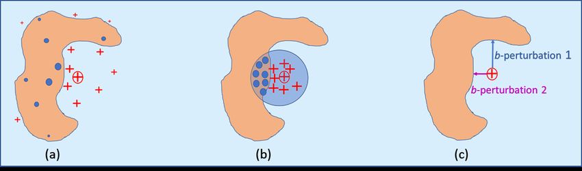
Figure 2. Excerpt from a CLEAR b-counterfactual report. In this example CLEAR uses multiple regression to explain a single prediction generated by an
MLP model trained on the Pima dataset
then there are q ≤ p×k −1 b-perturbations of x; changes in a feature are calculated by comparing the actual b-perturbations determined
value may not always imply a change of classification. in step 1 with the estimates calculated in step 5.
CLEAR compares each b-perturbation with an estimate of that 7. Iterate to best explanation. Because CLEAR produces fidelity
value, call it estimated b-perturbation, calculated using its local re- statistics, its parameters can be iteratively changed in order to
gression, to produce a counterfactual fidelity error, as follows: achieve a better trade-off between interpretability and fidelity. Rel-
evant parameters include the number of features/independent vari-
counterfactual fidelity error =
ables to consider and the use and number of quadratic or interac-
| estimated b-perturbation − b-perturbation | tion terms. Figure 2 shows excerpts from a CLEAR report.
Henceforth these will be referred to simply as ’fidelity errors’. 8. CLEAR also provides the option of adding x’s b-counterfactuals,
CLEAR generates an explanation of prediction y for observation x minf (x), to x’s neighbourhood dataset. The b-counterfactuals are
by the following steps: weighted and act as soft constraints on CLEAR’s subsequent re-
gression. Algorithms 1 and 2 outline the entire process.
1. Determine x’s b-perturbations. For each feature f, a separate one-
dimensional search is performed by querying m starting at x, and
progressively moving away from x by changing the value of f by Algorithm 1: CLEAR Algorithm
regular amounts, whilst keeping all other features constant. The input : t (training data), x,m,T
searches are constrained to a range of possible feature values. output: expl (set of explanations)
2. Generate labelled synthetic observations (default: 50,000 obser- S← Generate Synthetic Data(x,t,m)
vations). Data for numeric features is generated by sampling from for each target class tc do
a uniform distribution. Data for categorical features is generated for each feature f do
by sampling in proportion to the frequencies found in the train- w ← Find Counterfactuals(x,m)
ing set. The synthetic observations are labelled by being passed end
through m. Ntc ← Balanced Neighbourhood(S, x, m)
3. Create a balanced neighbourhood dataset (default is 200 observa- Optional: Ntc ← Ntc ∪ w
tions). Synthetic observations that are near to x (Euclidean dis- r ←Find Regression Equations(Ntc , x)
tance) are selected with the objective of achieving a dense cloud w0 ← Estimate Counterfactuals(r,x)
of points between x and the nearest points just beyond m’s deci- e ← Calculate Fidelity(w,w’,T)
sion boundaries (Figure 1). For this, the neighbourhood data is se- return expltc =< w, w0 , r, e >
lected such that it is equally distributed across classes, i.e. approx- end
imately balanced. CLEAR was also evaluated using ’imbalanced’
neighbourhood data, where only the synthetic observations near-
Algorithm 2: Balanced Neighbourhood
est to x were selected. However, it was found this reduced fidelity
(see Figure 3). It might be thought that a balanced neighbourhood input : S (synthetic dataset), x,m
dataset should not be used when x is far from m’s decision bound- b1 , b2 (margins around decision boundary)
ary; as this would lead to a ’non-local’ explanation. But this misses output: N (neighbourhood dataset)
the point that a satisfactory explanation is counterfactual, and that n ← 200
the required locality therefore extends from x to data points just for si ∈ S do
beyond m’s decision boundary. di ← Euclidean Distance (si , x)
4. Perform a step-wise regression on the neighbourhood dataset, un- yi ←m(si )
der the constraint that the regression curve should go through x. end
The regression can include second degree terms, interaction terms N1 ← n/3 members of {S} with lowest di s.t. 0 < yi ≤ b1
and indicator variables. CLEAR provides options for both multi- N2 ← n/3 members of {S} with lowest di s.t. b1 < yi ≤ b2
ple and logistic regression. A user can also specify terms that must N3 ← n/3 members of {S} with lowest di s.t. b2 < yi ≤ 1
be included in a regression. return N ← N1 ∪ N2 ∪ N3
5. Estimate the b-perturbations by substituting x’s b-counterfactual
values from minf (x), other than for feature f , into the regression Notice that for CLEAR an explanation (expl) is a tuple <
equation and calculating the value of f . See example below. w, w0 , r, e >, where w and w0 are b-perturbations (actual and es-
6. Measure the fidelity of the regression coefficients. Fidelity errors timated), r is a regression equation and e are fidelity errors.24th European Conference on Artificial Intelligence - ECAI 2020
Santiago de Compostela, Spain
Table 1. Comparison of % fidelity of CLEAR and LIME: the use of a balanced neighbourhood, centering and quadratic terms allow CLEAR, in general, to
achieve a considerably higher fidelity to b-counterfactuals than LIME, even without training with b-counterfactuals. Including training with b-counterfactuals
(optional step 8 of CLEAR method), % fidelity is further increased.
Adult Iris Pima Credit Breast
CLEAR- not using b-counterfactuals 80% ± 0.9 80% ± 1.0 57% ± 0.8 39% ± 1.3 54% ± 1.1
CLEAR- using b-counterfactuals 80% ± 0.8 99.8% ± 0.1 77% ± 0.8 55% ± 1.7 81% ± 1.3
LIME algorithms 26% ± 0.6 30% ± 0.3 20% ± 0.4 12% ± 0.5 14% ± 0.3
Example of using regression to estimate a b-perturbation: An ally provides options for the user to simplify the original regression,
MLP with a softmax activation function in the output layer was for example by reducing the number of terms, excluding interaction
trained on a subset of the UCI Pima Indians Diabetes dataset. The terms etc. CLEAR then enables the user to see the resulting fall in fi-
MLP calculated a probability of 0.69 for x belonging to class 1 delity, putting the user in control of the interpretability/fidelity trade-
(having diabetes). CLEAR generated the logistic regression equation off. Figure 3 illustrates how fidelity is reduced by excluding both
T
(1 + ew x )−1 = 0.69 where: quadratic and interaction terms; notice that even both are excluded,
CLEAR’s fidelity is much higher than LIME’s.
wT x = −0.8 + 1.73 Glucose + 0.25 BloodP ressure
+0.31 Glucose2
4 Experimental Results
Let the decision boundary be P (x ∈ class 1) = 0.5. Thus, x
is on the boundary when wT x = 0. The estimated b-perturbation Experiments were carried out with five UCI datasets: Pima Indians
for Glucose is obtained by substituting into the regression equation: Diabetes (with 8 numeric features), Iris (4 numeric features), Default
wT x = 0 and the value of BloodPressure in x: of Credit Card Clients (20 numeric features, 3 categorical), and sub-
−0.31 Glucose2 + 1.73 Glucose − .04 = 0 sets of Adult (with 2 numeric features, 5 categorical features), and
Solving this equation, CLEAR selects the root equal to 0.025 as Breast Cancer Wisconsin (9 numeric features). For the Adult dataset,
being closest to the original value of Glucose in x. The original some of the categorical features values were merged and features
value for Glucose was 0.537 and hence the estimated b-perturbation with little predictive power were removed. With the Breast Cancer
is -0.512. The actual b-perturbation (step 1) for Glucose to achieve a dataset only the mean value features were kept. For reproducibility,
probability of 0.5 of being in class 1 was -0.557; hence, the fidelity the code for pre-processing the data is included with the CLEAR
error was 0.045. prototype on GitHub.
For the Iris dataset, a support vector machine (SVM) with RBF
A CLEAR prototype has been developed in Python3 . CLEAR can kernel was trained using the scikit-learn library. For each of the other
be run either in batch mode on a test set or it can explain the pre- datasets, an MLP with a softmax output layer was trained using Ten-
diction of a single observation. In batch mode, CLEAR reports the sorflow. Each dataset was partitioned into a training dataset (used to
proportion of its estimated b-counterfactuals that have a fidelity error train the SVM or MLP, and to set the parameters used to generate
lower than a user-specified error threshold T, as follows: synthetic data for CLEAR) and a test dataset (out of which 100 ob-
Definition 5.3 (% fidelity): A b-perturbation is said to be feasible if servations were selected for calculating the % fidelity of CLEAR and
the resulting feature value is within the range of values found in m’s LIME). Experiments were carried out with different test sets, with
training set. The percentage fidelity given a batch and error threshold each experiment being repeated 20 times for different generated syn-
T is the number of b-perturbations with fidelity error smaller than T thetic data. The experiments were carried out on a Windows i7-8700
divided by the number of feasible b-perturbations. 3.2GHz PC. A single run of a 100 observations took 40-80 minutes,
Both fidelity and interpretability are critical for a successful ex- depending on the dataset.
planation. An ’interpretable explanation’ that is of poor fidelity is In order to enable comparisons with LIME, CLEAR includes an
not an explanation, it is just misinformation. Yet, in order to achieve option to run the LIME algorithms for creating synthetic data and
high levels of fidelity, a CLEAR regression may need to include a generating regression equations. CLEAR then takes the regression
large number of terms, including 2nd degree and interaction vari- equations and calculates the corresponding b-counterfactuals and
ables. A criticism of CLEAR might then be that whilst its regres- fidelity errors. It might be objected that it is unfair to evaluate LIME
sion equations are interpretable to data scientists, they may not be on its counterfactual fidelity, as it was not created for this purpose.
interpretable to lay people. However CLEAR’s HTML reports are But if you accept Woodward and Miller’s requirements for a satisfac-
interactive, providing an option to simplify the representation of its tory explanation, then counterfactual fidelity is an appropriate metric.
equations. Consider Figure 2, if a user was primarily interested in
the effects of Glucose and BMI, then CLEAR can substitute the val- CLEAR’s regressions are significantly better than LIME’s. The
ues of the other features leading to the full regression equation being best results are obtained by including b-counterfactuals in the neigh-
re-expressed as: bourhood datasets (step 8 of the CLEAR method). Overall, the best
configuration comprised: using balanced neighbourhood data, forc-
wT x = 0.46 + 0.3 Glucose + 0.18 BM I − 0.05 BM I 2 ing the regression curve to go through x (i.e. ’centering’), including
This equation helps to explain the b-counterfactuals, for example it both quadratic and interaction terms, and using logistic regression for
shows why observation 1’s classification is more easily ’flipped’ by Pima and Breast Cancer and multiple regression for Iris, Adult and
changing the value of Glucose rather than BMI. CLEAR addition- Credit datasets. Unless otherwise stated % fidelity is for the error
threshold T = 0.25. Table 1 compares the % fidelity of CLEAR and
3 https://github.com/ClearExplanationsAI LIME (i.e. using LIME’s algorithms for generating synthetic data24th European Conference on Artificial Intelligence - ECAI 2020
Santiago de Compostela, Spain
Figure 3. Comparison of fidelity with different configurations. Fidelity is reduced when any of the above changes are made to the best configuration. The
changes include:’Imbalanced neighbourhood’ = ’using best configuration but with imbalanced neighbourhood datasets’, and ’LIME’ = ’using the LIME
algorithms’. Notice the benefits of CLEAR using a balanced neighbourhood dataset. Also, when CLEAR has ’no quadratic and interaction terms’, it is still
significantly more faithful than LIME.
and performing the regression). This used LIME’s default parame- used a maximum of 14 independent variables.
ter values except for the following beneficial changes: the number CLEAR’s fidelity was sharply improved by adding x’s b-
of synthetic data points was increased to 15,000 (further increases counterfactuals to its neighbourhood datasets. In the previous ex-
did not improve fidelity), the data was not discretized, a maximum periments, CLEAR created a neighbourhood dataset of at least 200
of 14 features were allowed, several kernel widths in the range from synthetic observations, each being given a weighting of 1. This was
1.5 to 4 were evaluated. By contrast, CLEAR was run with its best now altered so that each b-counterfactual identified in step 1 was
configuration and with 14 features. As an example of LIME’s per- added and given a weighting of 10. For example, for the Pima
formance: with the Credit dataset, the adjusted R2 averaged ≈ 0.7, dataset, an average of ≈3 b-counterfactuals were added to each
the classification of the test set observations was over 94% correct. neighbourhood dataset. The consequent improvement in fidelity in-
However, the absolute error between y and LIME’s estimate of y was dicates as expected that adding these weighted data points results in
8% (e.g. the MLP forecast P (x ∈ class 1) = 0.4, while LIME es- a dataset capable of representing better the relevant neighbourhood,
timated it at 0.48) and this by itself would lead to large errors when with CLEAR being able to provide a regression equation that is more
calculating how much a single feature needs to change for y to reach faithful to b-counterfactuals.
the decision boundary. LIME’s fidelity of only 12%, illustrates that
CLEAR’s measure of fidelity is far more demanding than just clas-
sification accuracy. Of course, LIME’s poor fidelity was due, in part, 5 Conclusion and Future Work
to its kernel failing to isolate the appropriate neighbourhood datasets
CLEAR satisfies the requirement that satisfactory local explanations
necessary for calculating b-counterfactuals accurately.
should include statements of key counterfactual cases. CLEAR ex-
Table 2 shows how CLEAR’s fidelity (not using b-counterfactuals)
plains a prediction y for data point x by stating x’s b-counterfactuals
varied with the maximum ’number of independent variables’ allowed
and providing a regression equation. The regression shows the pat-
in a regression. At first, fidelity sharply improves but then plateaus.
terns of counterfactual dependencies in a neighbourhood that in-
Despite CLEAR’s regression fitting the neighbourhood data well,
cludes both x and the b-counterfactual data points. CLEAR rep-
a significant number of the estimated b-counterfactuals have large fi-
resents a significant improvement both on LIME and on just us-
delity errors. For example, in one of the experiments with the Adult
ing b-counterfactuals. Crucial to CLEAR’s performance is the abil-
dataset where the multiple regression did not center the data, the av-
ity to generate relevant neighbourhood data bounded by its b-
erage adjusted R2 was 0.97, classification accuracy 98% but the %
counterfactuals. Adding these to x’s neighbourhood led to sharp fi-
fidelity error < 0.25 was 59%. This points to a more general problem:
delity improvements. Another key feature of CLEAR is that it reports
sometimes the neighbourhood datasets do not represent the regions
on its own fidelity. Any local explanation system will be fallible, and
of its feature space that are central for its explanations. With CLEAR,
it is critical with high-value decisions that the user knows if they can
this discrepancy can at least be measured.
trust an explanation.
There is considerable scope for further developing CLEAR. These
Table 2. Variation of % fidelity with the choice of number of variables
include (i) the neighbourhood selection algorithms could be further
enhanced. Other data points could also be added, for example b-
No. Adult Iris PIMA Credit Breast
counterfactuals involving changes to multiple features. A user might
also include some perturbations that are important to their project.
8 35% 50% 42% 27% 43%
CLEAR could guide this process by reporting regression and fidelity
11 76% 62% 53% 38% 46%
14 80% 80% 57% 39% 54% statistics. And step 8 of the CLEAR algorithm could be replaced
17 78% n/a 59% 40% 55% by increasingly complex and more sophisticated learning algorithms.
20 78% n/a 62% 39% 56% Constructing neighbourhood datasets in this way would seem a bet-
ter approach than randomly generating data points and then selecting
CLEAR was tested in a variety of configurations. These included those closest to x (ii) the search algorithm for actual b-perturbations
the best configuration, and configurations where a single option was in step 1 of the CLEAR algorithm could be replaced by a more com-
altered from the default, e.g. by using a imbalanced neighbourhood putationally efficient algorithm (iii). CLEAR should be evaluated in
of points nearest to x. Figure 3 displays the results when CLEAR practice in the context of comprehensibility studies.24th European Conference on Artificial Intelligence - ECAI 2020
Santiago de Compostela, Spain
REFERENCES
[1] Robert Andrews, Joachim Diederich, and Alan B. Tickle, ‘Survey
and critique of techniques for extracting rules from trained artifi-
cial neural networks’, Knowledge-Based Systems, 8(6), 373–389,
(December 1995).
[2] Elaine Angelino, Nicholas Larus-Stone, Daniel Alabi, Margo
Seltzer, and Cynthia Rudin, ‘Learning certifiably optimal rule
lists for categorical data’, Journal of Machine Learning Re-
search, 18, 234:1–234:78, (2017).
[3] David Bau, Bolei Zhou, Aditya Khosla, Aude Oliva, and An-
tonio Torralba, ‘Network dissection: Quantifying interpretability
of deep visual representations’, In Proc. CVPR 2017, Honolulu,
USA, (2017).
[4] Mark W. Craven and Jude W. Shavlik, ‘Extracting tree-structured
representations of trained networks’, in Proc. NIPS 1995, pp. 24–
30. MIT Press, (1995).
[5] Zoubin Ghahramani, ‘Probabilistic machine learning and artifi-
cial intelligence’, Nature, 521(7553), 452–459, (2015).
[6] Riccardo Guidotti, Anna Monreale, Franco Turini, Dino Pe-
dreschi, and Fosca Giannotti, ‘A survey of methods for explain-
ing black box models’, CoRR, abs/1802.01933, (2018).
[7] Patrick Hall, Navdeep Gill, Megan Kurka, and Wen Phan.
Machine learning interpretability with H2O driverless
AI, 2017. URL: http://docs.h2o.ai/ driverless-ai/latest-
stable/docs/booklets/MLIBooklet.pdf.
[8] Irina Higgins, Loic Matthey, Arka Pal, Christopher Burgess,
Xavier Glorot, Matthew Botvinick, Shakir Mohamed, and
Alexander Lerchner, ‘beta-vae: Learning basic visual concepts
with a constrained variational framework.’, ICLR, 2(5), 6,
(2017).
[9] Linwei Hu, Jie Chen, Vijayan N. Nair, and Agus Sudjianto, ‘Lo-
cally interpretable models and effects based on supervised parti-
tioning (LIME-SUP)’, CoRR, abs/1806.00663, (2018).
[10] Henrik Jacobsson, ‘Rule extraction from recurrent neural net-
works: A taxonomy and review’, Neural Computation, 17(6),
1223–1263, (June 2005).
[11] Scott M Lundberg and Su-In Lee, ‘A unified approach to inter-
preting model predictions’, in Advances in Neural Information
Processing Systems, pp. 4765–4774, (2017).
[12] Tim Miller, ‘Contrastive explanation: A structural-model ap-
proach’, arXiv preprint arXiv:1811.03163, (2018).
[13] Tim Miller, ‘Explanation in artificial intelligence: Insights from
the social sciences’, Artificial Intelligence, (2018).
[14] Saumitra Mishra, Bob L Sturm, and Simon Dixon, ‘Local inter-
pretable model-agnostic explanations for music content analy-
sis.’, in ISMIR, pp. 537–543, (2017).
[15] Brent Mittelstadt, Chris Russell, and Sandra Wachter, ‘Explain-
ing explanations in AI’, in In Proc. Conference on Fairness,
Accountability, and Transparency, FAT’19, pp. 279–288, New
York, USA, (2019).
[16] Judea Pearl, Causality: Models, Reasoning and Inference, Cam-
bridge University Press, New York, NY, USA, 2nd edn., 2009.
[17] Marco Tulio Ribeiro, Sameer Singh, and Carlos Guestrin, ‘Why
should i trust you? explaining the predictions of any classifier’, in
Proc. ACM SIGKDD 2016, KDD ’16, pp. 1135–1144, New York,
NY, USA, (2016). ACM.
[18] Marco Tulio Ribeiro, Sameer Singh, and Carlos Guestrin, ‘An-
chors: High-precision model-agnostic explanations’, in Thirty-
Second AAAI Conference on Artificial Intelligence, (2018).
[19] Son N. Tran and Artur S. d’Avila Garcez, ‘Deep logic networks:
Inserting and extracting knowledge from deep belief networks’,
IEEE Transactions on Neural Networks and Learning Systems,
29(2), 246–258, (2018).
[20] Sandra Wachter, Brent D. Mittelstadt, and Chris Russell, ‘Coun-
terfactual explanations without opening the black box: Auto-
mated decisions and the GDPR’, CoRR, abs/1711.00399, (2017).
[21] Qinglong Wang, Kaixuan Zhang, Alexander G. Ororbia, II,
Xinyu Xing, Xue Liu, and C. Lee Giles, ‘An empirical evalua-
tion of rule extraction from recurrent neural networks’, Neural
Computation, 30(9), 2568–2591, (September 2018).
[22] J. Woodward, Making things happen: a theory of causal expla-
nation, Oxford University Press, Oxford, England, 2003.You can also read