MIKE 3 Wave Model FM Hydrodynamic Module - User Guide
←
→
Page content transcription
If your browser does not render page correctly, please read the page content below

MIKE 3 Wave Model FM

                                   Hydrodynamic Module

                                             User Guide

Powering Water Decisions                        MIKE 2021
2
PLEASE NOTE

COPYRIGHT                  This document refers to proprietary computer software which is pro-
                           tected by copyright. All rights are reserved. Copying or other repro-
                           duction of this manual or the related programs is prohibited without
                           prior written consent of DHI A/S (hereinafter referred to as “DHI”).
                           For details please refer to your 'DHI Software Licence Agreement'.

LIMITED LIABILITY          The liability of DHI is limited as specified in your DHI Software
                           Licence Agreement:

                           In no event shall DHI or its representatives (agents and suppliers)
                           be liable for any damages whatsoever including, without limitation,
                           special, indirect, incidental or consequential damages or damages
                           for loss of business profits or savings, business interruption, loss of
                           business information or other pecuniary loss arising in connection
                           with the Agreement, e.g. out of Licensee's use of or the inability to
                           use the Software, even if DHI has been advised of the possibility of
                           such damages.

                           This limitation shall apply to claims of personal injury to the extent
                           permitted by law. Some jurisdictions do not allow the exclusion or
                           limitation of liability for consequential, special, indirect, incidental
                           damages and, accordingly, some portions of these limitations may
                           not apply.

                           Notwithstanding the above, DHI's total liability (whether in contract,
                           tort, including negligence, or otherwise) under or in connection with
                           the Agreement shall in aggregate during the term not exceed the
                           lesser of EUR 10.000 or the fees paid by Licensee under the Agree-
                           ment during the 12 months' period previous to the event giving rise
                           to a claim.

                           Licensee acknowledge that the liability limitations and exclusions
                           set out in the Agreement reflect the allocation of risk negotiated and
                           agreed by the parties and that DHI would not enter into the Agree-
                           ment without these limitations and exclusions on its liability. These
                           limitations and exclusions will apply notwithstanding any failure of
                           essential purpose of any limited remedy.

Powering Water Decisions                                                                              3
4 MIKE 3 Wave Model FM - © DHI A/S
CONTENTS

1     About This Guide . . . . . . . . . . . . . . . . . . . . . . . . . . . . . . . . . . .                                                             9
      1.1     Purpose . . . . . . . . . .     .   .   .   .   .   .   .   .   .   .   .   .   .   .   .   .   .   .   .   .   .   .   .   .   .   .   . 9
      1.2     Assumed User Background         .   .   .   .   .   .   .   .   .   .   .   .   .   .   .   .   .   .   .   .   .   .   .   .   .   .   . 9
      1.3     General Editor Layout . . .     .   .   .   .   .   .   .   .   .   .   .   .   .   .   .   .   .   .   .   .   .   .   .   .   .   .   . 9
              1.3.1   Navigation tree . .     .   .   .   .   .   .   .   .   .   .   .   .   .   .   .   .   .   .   .   .   .   .   .   .   .   .   . 9
              1.3.2   Editor window . . .     .   .   .   .   .   .   .   .   .   .   .   .   .   .   .   .   .   .   .   .   .   .   .   .   .   .   . 9
              1.3.3   Validation window .     .   .   .   .   .   .   .   .   .   .   .   .   .   .   .   .   .   .   .   .   .   .   .   .   .   .   . 10
      1.4     Online Help . . . . . . . . .   .   .   .   .   .   .   .   .   .   .   .   .   .   .   .   .   .   .   .   .   .   .   .   .   .   .   . 10
2     Introduction . . . . . . . . . . . . . . . . . . . . . . . . . . . . . . . . . . . . . . 11
      2.1     Short Description . . . . . . . . . . . . . . . . . . . . . . . . . . . . . . . . . 11
      2.2     Application Areas . . . . . . . . . . . . . . . . . . . . . . . . . . . . . . . . . 11
3     Getting Started . . . . . . . . . . . . . . . . . . . . . . . . . . . . . . . . . . . . 13
      3.1     Defining and Limiting the Wave Problem . . .                        .   .   .   .   .   .   .   .   .   .   .   .   .   .   .   .   .   .   13
              3.1.1     Identify the wave problem . . . . .                       .   .   .   .   .   .   .   .   .   .   .   .   .   .   .   .   .   .   13
              3.1.2     Check MIKE 3 Wave FM capabilities                         .   .   .   .   .   .   .   .   .   .   .   .   .   .   .   .   .   .   14
              3.1.3     Define computational domain . . . .                       .   .   .   .   .   .   .   .   .   .   .   .   .   .   .   .   .   .   14
              3.1.4     Check computer resources . . . . .                        .   .   .   .   .   .   .   .   .   .   .   .   .   .   .   .   .   .   14
      3.2     Collecting Data . . . . . . . . . . . . . . . .                     .   .   .   .   .   .   .   .   .   .   .   .   .   .   .   .   .   .   14
      3.3     Setting up the Model . . . . . . . . . . . . .                      .   .   .   .   .   .   .   .   .   .   .   .   .   .   .   .   .   .   15
              3.3.1     What does it mean . . . . . . . . .                       .   .   .   .   .   .   .   .   .   .   .   .   .   .   .   .   .   .   15
              3.3.2     Mesh and bathymetry . . . . . . . .                       .   .   .   .   .   .   .   .   .   .   .   .   .   .   .   .   .   .   15
              3.3.3     Porosity . . . . . . . . . . . . . . .                    .   .   .   .   .   .   .   .   .   .   .   .   .   .   .   .   .   .   15
              3.3.4     Sponge layer . . . . . . . . . . . .                      .   .   .   .   .   .   .   .   .   .   .   .   .   .   .   .   .   .   16
              3.3.5     Wave data . . . . . . . . . . . . .                       .   .   .   .   .   .   .   .   .   .   .   .   .   .   .   .   .   .   16
      3.4     Calibrating and Verifying the Model . . . . .                       .   .   .   .   .   .   .   .   .   .   .   .   .   .   .   .   .   .   16
              3.4.1     Purpose . . . . . . . . . . . . . . .                     .   .   .   .   .   .   .   .   .   .   .   .   .   .   .   .   .   .   16
              3.4.2     Verification . . . . . . . . . . . . .                    .   .   .   .   .   .   .   .   .   .   .   .   .   .   .   .   .   .   16
              3.4.3     Calibration parameters . . . . . . .                      .   .   .   .   .   .   .   .   .   .   .   .   .   .   .   .   .   .   16
      3.5     Running the Production Simulations . . . . .                        .   .   .   .   .   .   .   .   .   .   .   .   .   .   .   .   .   .   17
      3.6     Presenting the Results . . . . . . . . . . . .                      .   .   .   .   .   .   .   .   .   .   .   .   .   .   .   .   .   .   17
4     Examples      . . . . . . . . . . . . . . .         .   .   .   .   .   .   .   .   .   .   .   .   .   .   .   .   .   .   .   .   .   .   .   .   19
      4.1     General . . . . . . . . . . . . . .         .   .   .   .   .   .   .   .   .   .   .   .   .   .   .   .   .   .   .   .   .   .   .   .   19
      4.2     Ronne Harbour . . . . . . . . . .           .   .   .   .   .   .   .   .   .   .   .   .   .   .   .   .   .   .   .   .   .   .   .   .   19
              4.2.1   Purpose of the example              .   .   .   .   .   .   .   .   .   .   .   .   .   .   .   .   .   .   .   .   .   .   .   .   19
              4.2.2   Model setup . . . . . . .           .   .   .   .   .   .   .   .   .   .   .   .   .   .   .   .   .   .   .   .   .   .   .   .   20
              4.2.3   Model results . . . . . .           .   .   .   .   .   .   .   .   .   .   .   .   .   .   .   .   .   .   .   .   .   .   .   .   23

Powering Water Decisions                                                                                                                                   5
4.2.4    List of data and specification files              .   .   .   .   .   .   .   .   .   .   .   .   .   .   .   .   .   .   .   24
    4.3   Breaking Waves on a Plane Beach . . . .                    .   .   .   .   .   .   .   .   .   .   .   .   .   .   .   .   .   .   .   24
          4.3.1    Purpose of the example . . . . .                  .   .   .   .   .   .   .   .   .   .   .   .   .   .   .   .   .   .   .   24
          4.3.2    Model setup . . . . . . . . . . .                 .   .   .   .   .   .   .   .   .   .   .   .   .   .   .   .   .   .   .   24
          4.3.3    Model results . . . . . . . . . . .               .   .   .   .   .   .   .   .   .   .   .   .   .   .   .   .   .   .   .   25
          4.3.4    List of data and specification files              .   .   .   .   .   .   .   .   .   .   .   .   .   .   .   .   .   .   .   28
    4.4   Breakwater Overtopping . . . . . . . . . .                 .   .   .   .   .   .   .   .   .   .   .   .   .   .   .   .   .   .   .   28
          4.4.1    Purpose of the example . . . . .                  .   .   .   .   .   .   .   .   .   .   .   .   .   .   .   .   .   .   .   28
          4.4.2    Model setup . . . . . . . . . . .                 .   .   .   .   .   .   .   .   .   .   .   .   .   .   .   .   .   .   .   28
          4.4.3    Model results . . . . . . . . . . .               .   .   .   .   .   .   .   .   .   .   .   .   .   .   .   .   .   .   .   30
          4.4.4    List of data and specification files              .   .   .   .   .   .   .   .   .   .   .   .   .   .   .   .   .   .   .   31
    4.5   Coastal Flooding in Capbreton . . . . . .                  .   .   .   .   .   .   .   .   .   .   .   .   .   .   .   .   .   .   .   32
          4.5.1    Purpose of the example . . . . .                  .   .   .   .   .   .   .   .   .   .   .   .   .   .   .   .   .   .   .   32
          4.5.2    Model setup . . . . . . . . . . .                 .   .   .   .   .   .   .   .   .   .   .   .   .   .   .   .   .   .   .   33
          4.5.3    Model results . . . . . . . . . . .               .   .   .   .   .   .   .   .   .   .   .   .   .   .   .   .   .   .   .   34
          4.5.4    List of data and specification files              .   .   .   .   .   .   .   .   .   .   .   .   .   .   .   .   .   .   .   38
5   BASIC PARAMETERS . . . . . . . . . . . . . . . . . . . . . . . . . . . . . . . . 39
    5.1   Domain . . . . . . . . . . . .     .   .   .   .   .   .   .   .   .   .   .   .   .   .   .   .   .   .   .   .   .   .   .   .   .   39
          5.1.1   Mesh and bathymetry        .   .   .   .   .   .   .   .   .   .   .   .   .   .   .   .   .   .   .   .   .   .   .   .   .   40
          5.1.2   Domain specification .     .   .   .   .   .   .   .   .   .   .   .   .   .   .   .   .   .   .   .   .   .   .   .   .   .   42
          5.1.3   Vertical mesh . . . . .    .   .   .   .   .   .   .   .   .   .   .   .   .   .   .   .   .   .   .   .   .   .   .   .   .   43
          5.1.4   Boundary names . . .       .   .   .   .   .   .   .   .   .   .   .   .   .   .   .   .   .   .   .   .   .   .   .   .   .   48
    5.2   Time . . . . . . . . . . . . . .   .   .   .   .   .   .   .   .   .   .   .   .   .   .   .   .   .   .   .   .   .   .   .   .   .   48
          5.2.1   Remarks and hints . .      .   .   .   .   .   .   .   .   .   .   .   .   .   .   .   .   .   .   .   .   .   .   .   .   .   49
6   HYDRODYNAMIC MODULE . . . . . . . . . . . . . . . . . . . . . . . . . . . . 51
    6.1   Solution Technique . . . . . . .       .   .   .   .   .   .   .   .   .   .   .   .   .   .   .   .   .   .   .   .   .   .   .   .   51
          6.1.1     CFL number . . . . . .       .   .   .   .   .   .   .   .   .   .   .   .   .   .   .   .   .   .   .   .   .   .   .   .   52
          6.1.2     Remarks and hints . . .      .   .   .   .   .   .   .   .   .   .   .   .   .   .   .   .   .   .   .   .   .   .   .   .   52
    6.2   Depth Correction . . . . . . . . .     .   .   .   .   .   .   .   .   .   .   .   .   .   .   .   .   .   .   .   .   .   .   .   .   53
          6.2.1     General description . .      .   .   .   .   .   .   .   .   .   .   .   .   .   .   .   .   .   .   .   .   .   .   .   .   53
    6.3   Flood and Dry . . . . . . . . . .      .   .   .   .   .   .   .   .   .   .   .   .   .   .   .   .   .   .   .   .   .   .   .   .   53
          6.3.1     General description . .      .   .   .   .   .   .   .   .   .   .   .   .   .   .   .   .   .   .   .   .   .   .   .   .   54
          6.3.2     Recommended values .         .   .   .   .   .   .   .   .   .   .   .   .   .   .   .   .   .   .   .   .   .   .   .   .   55
          6.3.3     Remarks and hints . . .      .   .   .   .   .   .   .   .   .   .   .   .   .   .   .   .   .   .   .   .   .   .   .   .   55
    6.4   Eddy Viscosity . . . . . . . . . .     .   .   .   .   .   .   .   .   .   .   .   .   .   .   .   .   .   .   .   .   .   .   .   .   55
          6.4.1     Horizontal eddy viscosity    .   .   .   .   .   .   .   .   .   .   .   .   .   .   .   .   .   .   .   .   .   .   .   .   55
          6.4.2     Vertical Eddy Viscosity .    .   .   .   .   .   .   .   .   .   .   .   .   .   .   .   .   .   .   .   .   .   .   .   .   56
          6.4.3     General description . .      .   .   .   .   .   .   .   .   .   .   .   .   .   .   .   .   .   .   .   .   .   .   .   .   57
          6.4.4     Recommended values .         .   .   .   .   .   .   .   .   .   .   .   .   .   .   .   .   .   .   .   .   .   .   .   .   58
          6.4.5     Remarks and hints . . .      .   .   .   .   .   .   .   .   .   .   .   .   .   .   .   .   .   .   .   .   .   .   .   .   58
    6.5   Bed Resistance . . . . . . . . .       .   .   .   .   .   .   .   .   .   .   .   .   .   .   .   .   .   .   .   .   .   .   .   .   58
          6.5.1     General description . .      .   .   .   .   .   .   .   .   .   .   .   .   .   .   .   .   .   .   .   .   .   .   .   .   59
          6.5.2     Recommended values .         .   .   .   .   .   .   .   .   .   .   .   .   .   .   .   .   .   .   .   .   .   .   .   .   59
          6.5.3     Remarks and hints . . .      .   .   .   .   .   .   .   .   .   .   .   .   .   .   .   .   .   .   .   .   .   .   .   .   60
    6.6   Coriolis Forcing . . . . . . . . .     .   .   .   .   .   .   .   .   .   .   .   .   .   .   .   .   .   .   .   .   .   .   .   .   60
          6.6.1     Remarks and hints . . .      .   .   .   .   .   .   .   .   .   .   .   .   .   .   .   .   .   .   .   .   .   .   .   .   60

6                                                                                MIKE 3 Wave Model FM - © DHI A/S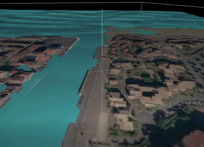
6.7     Porosity . . . . . . . . . . . . .   .   .   .   .   .   .   .   .   .   .   .   .   .   .   .   .   .   .   .   .   .   .   .   .   .   60
              6.7.1     General description . .    .   .   .   .   .   .   .   .   .   .   .   .   .   .   .   .   .   .   .   .   .   .   .   .   .   62
      6.8     Sponge Layer . . . . . . . . .       .   .   .   .   .   .   .   .   .   .   .   .   .   .   .   .   .   .   .   .   .   .   .   .   .   63
              6.8.1     General description . .    .   .   .   .   .   .   .   .   .   .   .   .   .   .   .   .   .   .   .   .   .   .   .   .   .   65
      6.9     Internal Wave Generation . . .       .   .   .   .   .   .   .   .   .   .   .   .   .   .   .   .   .   .   .   .   .   .   .   .   .   66
              6.9.1     Relaxation data . . . .    .   .   .   .   .   .   .   .   .   .   .   .   .   .   .   .   .   .   .   .   .   .   .   .   .   67
              6.9.2     Wave data . . . . . .      .   .   .   .   .   .   .   .   .   .   .   .   .   .   .   .   .   .   .   .   .   .   .   .   .   68
              6.9.3     Interpolation overlay .    .   .   .   .   .   .   .   .   .   .   .   .   .   .   .   .   .   .   .   .   .   .   .   .   .   73
              6.9.4     General description . .    .   .   .   .   .   .   .   .   .   .   .   .   .   .   .   .   .   .   .   .   .   .   .   .   .   74
      6.10    Initial Conditions . . . . . . . .   .   .   .   .   .   .   .   .   .   .   .   .   .   .   .   .   .   .   .   .   .   .   .   .   .   75
      6.11    Boundary Conditions . . . . . .      .   .   .   .   .   .   .   .   .   .   .   .   .   .   .   .   .   .   .   .   .   .   .   .   .   76
              6.11.1 Boundary specification        .   .   .   .   .   .   .   .   .   .   .   .   .   .   .   .   .   .   .   .   .   .   .   .   .   76
      6.12    Turbulence Module . . . . . . .      .   .   .   .   .   .   .   .   .   .   .   .   .   .   .   .   .   .   .   .   .   .   .   .   .   77
      6.13    Outputs . . . . . . . . . . . . .    .   .   .   .   .   .   .   .   .   .   .   .   .   .   .   .   .   .   .   .   .   .   .   .   .   77
              6.13.1 Geographical view . .         .   .   .   .   .   .   .   .   .   .   .   .   .   .   .   .   .   .   .   .   .   .   .   .   .   77
              6.13.2 Output specification . .      .   .   .   .   .   .   .   .   .   .   .   .   .   .   .   .   .   .   .   .   .   .   .   .   .   77
              6.13.3 Output items . . . . .        .   .   .   .   .   .   .   .   .   .   .   .   .   .   .   .   .   .   .   .   .   .   .   .   .   86
7     TURBULENCE MODULE . . . . . . . . . . . . . . . . . . . . . . . . . . . . . . 91
      7.1     Equation . . . . . . . . . . . .     .   .   .   .   .   .   .   .   .   .   .   .   .   .   .   .   .   .   .   .   .   .   .   .   .   91
      7.2     Solution Technique . . . . . . .     .   .   .   .   .   .   .   .   .   .   .   .   .   .   .   .   .   .   .   .   .   .   .   .   .   92
              7.2.1     Remarks and hints . .      .   .   .   .   .   .   .   .   .   .   .   .   .   .   .   .   .   .   .   .   .   .   .   .   .   92
      7.3     Dispersion . . . . . . . . . . .     .   .   .   .   .   .   .   .   .   .   .   .   .   .   .   .   .   .   .   .   .   .   .   .   .   93
      7.4     Initial Conditions . . . . . . . .   .   .   .   .   .   .   .   .   .   .   .   .   .   .   .   .   .   .   .   .   .   .   .   .   .   93
              7.4.1     Recommended values         .   .   .   .   .   .   .   .   .   .   .   .   .   .   .   .   .   .   .   .   .   .   .   .   .   94
8     LIST OF REFERENCES . . . . . . . . . . . . . . . . . . . . . . . . . . . . . . . 95

Index . . . . . . . . . . . . . . . . . . . . . . . . . . . . . . . . . . . . . . . . . . . . . 97

Powering Water Decisions                                                                                                                                7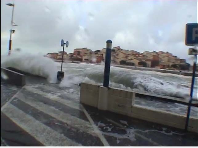
8 MIKE 3 Wave Model FM - © DHI A/S

Purpose

1         About This Guide

1.1       Purpose
                     The main purpose of this User Guide is to enable you to use MIKE 3 Wave
                     Model FM, Hydrodynamic Module, for determination and assessment of
                     wave dynamics in ports, harbours and coastal areas. The User Guide is com-
                     plemented by the Online Help.

1.2       Assumed User Background
                     Although the hydrodynamic module has been designed carefully with empha-
                     sis on a logical and user-friendly interface, and although the User Guide and
                     Online Help contains modelling procedures and a large amount of reference
                     material, common sense is always needed in any practical application.

                     In this case, “common sense” means a background in coastal hydraulics and
                     oceanography, which is sufficient for you to be able to check whether the
                     results are reasonable or not. This User Guide is not intended as a substitute
                     for a basic knowledge of the area in which you are working: Mathematical
                     modelling of hydraulic phenomena.

                     It is assumed that you are familiar with the basic elements of MIKE Zero: File
                     types and file editors, the Plot Composer, the MIKE Zero Toolbox, the Data
                     Viewer and the Mesh Generator. The documentation for these can by found
                     from the MIKE Zero Documentation Index.

1.3       General Editor Layout
                     The MIKE 3 Wave Model FM setup editor consists of three separate panes.

1.3.1     Navigation tree

                     To the left is a navigation tree, that shows the structure of the model setup
                     file, and is used to navigate through the separate sections of the file. By
                     selecting an item in this tree, the corresponding editor is shown in the central
                     pane of the setup editor.

1.3.2     Editor window

                     The editor for the selected section is shown in the central pane. The content
                     of this editor is specific for the selected section, and might contain several
                     property pages.

                     For sections containing spatial data - e.g. internal wave generation, bounda-
                     ries and output - a geographic view showing the location of the relevant items

Powering Water Decisions                                                                            9
About This Guide
will be available. The current navigation mode is selected in the bottom of this
view, it can be zoomed in, zoomed out or recentered. A context menu is avail-
able from which the user can select to show the bathymetry or the mesh and
to show the legend. From this context menu it is also possible to navigate to
the previous and next zoom extent and to zoom to full extent. If the context
menu is opened on an item - e.g. an internal wave generation zone - it is also
possible to jump to this item’s editor.
Further options may be available in the context menu depending on the sec-
tion being edited.
1.3.3 Validation window
The bottom pane of the editor shows possible validation errors, and is
dynamically updated to reflect the current status of the setup specifications.
By double-clicking on an error in this window, the editor in which this error
occurs will be selected.
1.4 Online Help
The Online Help can be activated in several ways, depending on the user's
requirement:
F1-key seeking help on a specific activated dialog:
To access the help associated with a specific dialog page, press the
F1-key on the keyboard after opening the editor and activating the spe-
cific property page.
Open the On-line Help system for browsing manually after a specific help
page:
Open the On-line Help system by selecting “Help Topics” in the main
menu bar.
10 MIKE 3 Wave Model FM - © DHI A/SShort Description
2 Introduction
MIKE 3 Wave Model FM is a non-hydrostatic wave model that is capable of
simulating wave processes from deep water to nearshore. This model
enhances the versatility and applicability of the MIKE software in offshore,
coastal and port engineering.
2.1 Short Description
MIKE 3 Wave Model FM is a phase-resolving wave model based on the 3D
Navier-Stokes equations and with the free surface described by a height
function. The numerical techniques applied are based on an unstructured
(flexible) mesh approach.
2.2 Application Areas
The model is to be applied in the following areas:
Ports and terminals
– Wave agitation caused by short and long waves
– Input to dynamic ship mooring analysis (MIKE 21 MA)
Coastal areas
– Non-linear wave transformation
– Surf and swash zone hydrodynamics
– Wave breaking and run-up
– Coastal flooding
– Tsunami (transient) modelling
Coastal structures
– Wave overtopping
– Wave transmission (and reflection) through porous structures
Offshore environments
– Transformation of steep non-linear waves
– 3D wave kinematics for structural load calculations
Powering Water Decisions 11Introduction 12 MIKE 3 Wave Model FM - © DHI A/S
Defining and Limiting the Wave Problem
3 Getting Started
The purpose of this chapter is to give you a general check list, which you can
use for determination and assessment of wave dynamics in ports, harbours
and coastal areas using MIKE 3 Wave Model FM.
The work will normally consist of the six tasks listed below:
1. Defining and limiting the wave problem
2. Collecting data
3. Setting up the model
4. Calibrating and verifying the model
5. Running the production simulations
6. Presenting the results
Each of these six tasks are described for a "general wave study" in the follow-
ing sections. For your particular study only some of the tasks might be rele-
vant. Please note that whenever a word is written in italics it is included as an
entry in the Online Help and in the Reference Manual.
3.1 Defining and Limiting the Wave Problem
3.1.1 Identify the wave problem
When preparing to do a wave study you have to assess the following before
you start to set up the model:
What are the "wave conditions" under consideration in the "area of inter-
est"?
What are the "important wave phenomena"?
The following phenomena should be taken into consideration:
– Shoaling
– Refraction
– Diffraction
– Partial reflection/transmission
– Bottom dissipation
– Wave breaking
– Run-up
– Wind-wave generation
– Frequency spreading
– Directional spreading
– Wave-wave interaction
– Wave-current interaction
Powering Water Decisions 13Getting Started
MIKE 3 Wave Model FM can handle these phenomena with the exception of
wind-wave generation.
3.1.2 Check MIKE 3 Wave FM capabilities
Next, check if MIKE 3 Wave Model FM is able to solve your problem. This you
can do by turning to Section 2, which gives a short description of MIKE 3
Wave Model FM and an overview of the type of applications for which MIKE 3
Wave Model FM can be used, and by consulting the Scientific Documenta-
tion.
3.1.3 Define computational domain
Draw up your model domain on a sea chart showing the area of interest and
the area of influence. This is normally an iterative process as on one hand
you should keep the model domain as small as possible, while on the other
hand you have to include the total area of influence. You also have to con-
sider the location of porous structures.
The choice of the discrete resolution in the geographic and spectral space
depends on the wave conditions for which simulations are to be performed
and on the bathymetry and forcing fields (current, water level):
Discrete resolution in the geographical space must be selected to pro-
vide adequate resolution of the bathymetry.
Discrete resolution in the geographical space and the vertical space
must be selected to provide adequate resolution at the wave field under
consideration.
3.1.4 Check computer resources
Finally, before you start to set up the model, you should check that you are
not requesting unrealistic computer resources:
The CPU time required should be estimated.
The Disk Space required should be estimated.
It is recommended to run the MIKE 3 Wave Model FM examples included in
the installation for assessment of the computational speed on your PC and to
assess the disk space consumption.
3.2 Collecting Data
This task may take a long time if, for example, you have to initiate a monitor-
ing program. Alternatively it may be carried out very quickly if you are able to
14 MIKE 3 Wave Model FM - © DHI A/SSetting up the Model
use existing data which are immediately available. In all cases the following
data should be collected:
Bathymetric data such as charts from local surveys or, for example, from
the Hydrographic Office, UK, or MIKE C-MAP
Wave data, which might be measurements (existing or planned specifi-
cally for your model), observations, wave statistics, etc.
Information on type of structures for assessment of the reflection proper-
ties
Calibration and validation data; these might be measured wave parame-
ters at selected locations, observations, etc.
3.3 Setting up the Model
3.3.1 What does it mean
"Setting up the model" is actually another way of saying transforming real
world events and data into a format which can be understood by the numeri-
cal model MIKE 3 Wave Model FM. Thus generally speaking, all the data col-
lected have to be resolved on the spatial grid selected.
3.3.2 Mesh and bathymetry
Providing MIKE 3 Wave Model FM with a suitable mesh and bathymetry is
essential for obtaining reliable results from your model. Setting up the mesh
includes the appropriate selection of the area to be modelled, adequate reso-
lution of the bathymetry and wave field under consideration and definition of
codes for specification of location of porosity zones and sponge layers. Fur-
thermore, the resolution in the geographical space must also be selected with
respect to stability considerations.
Describing the water depth in your defined model domain is one of the most
important tasks in the modelling process. A few hours less spent in generat-
ing the mesh covering the bathymetry may later on mean extra days spent in
the calibration process.
The mesh file including your bathymetry is generated by MIKE Zero Mesh
Generator, which is a tool for the generation and handling of unstructured
meshes, including the definition and editing of boundaries. If a structured
mesh consisting of quadrilateral elements is used, the mesh can also be gen-
erated using the MIKE Zero Bathymetry Editor.
3.3.3 Porosity
The location of the porous structures zones can be determined from the
boundary information.
Powering Water Decisions 15Getting Started
3.3.4 Sponge layer
The location of the sponge layers is can be determined from the boundary
information.
3.3.5 Wave data
In most cases you will force the model by waves generated inside the model
domain. The internal wave generation of waves allows you to absorb all
waves leaving the model domain (radiation type boundaries).
3.4 Calibrating and Verifying the Model
3.4.1 Purpose
Having completed all the tasks listed above you are ready to do the first time-
domain wave simulation and to start the calibration of the model. The pur-
pose of the calibration is to tune the model in order to reproduce
known/measured wave conditions. The calibrated/tuned model is then veri-
fied by running one or more simulations for which measurements are availa-
ble without changing any tuning parameters. This should ensure that
simulations can be made for any wave conditions similar to the calibration
and verification wave conditions with satisfactory results. However, you
should never use simulation results, whether verified or not, without checking
if they are reasonable or not.
3.4.2 Verification
The situations which you select for calibration and verification of the model
should cover the range of situations you wish to investigate in the production
runs. However, as you must have some measurements/observations against
which to calibrate and, as the measurements are often only available for short
periods, you may only have a few situations from which to choose. When you
have finished the calibration you can run one more simulation for which you
have measurements (or other data) without changing the calibration parame-
ters. If you then get a satisfactory agreement between the simulation results
and the measurements you can consider your calibration to be successful.
3.4.3 Calibration parameters
When you run your calibration run for the first time and compare the simula-
tion results to your measurements (or other information) you will, in many
cases, see differences between the two. The purpose of the calibration is
then to tune the model so that these differences become negligible. You can
change the following model specifications in order to reduce the differences:
16 MIKE 3 Wave Model FM - © DHI A/SRunning the Production Simulations
Wave conditions
Porosity
Bed resistance
Bathymetry
Recommendations on how the specification can be changed are given in the
Reference Manual.
3.5 Running the Production Simulations
As you have calibrated and verified the model you can get on to the "real"
work, that is doing your actual investigation. This will, in some cases, only
include a few runs.
3.6 Presenting the Results
Throughout a modelling study you are working with large amounts of data
and the best way of checking them is therefore to look at them graphically.
Only in a few cases, such as when you check your bathymetry along a
boundary or you want to compare simulation results to measurements in
selected locations, should you look at the individual numbers. Much empha-
sis has therefore been placed on the capabilities for graphical presentation in
MIKE Zero and it is an area which will be expanded and focused on even fur-
ther in future versions. Essentially, one plot gives more information than
scores of tables. A good way of presenting the model results is using contour
plots of e.g. the calculated wave disturbance coefficient by using the Plot
Composer or Result Viewer tool in MIKE Zero. Instantaneous pictures/videos
of the simulated surface elevations can also be generated. For 3D visualis-
ation MIKE Animator Plus is recommended.
Powering Water Decisions 17Getting Started 18 MIKE 3 Wave Model FM - © DHI A/S
General
4 Examples
4.1 General
One of the best ways of learning how to use a modelling system like MIKE 3
Wave Model FM is through practice. Therefore, examples have been
included which you can go through yourself and which you can modify, if you
like, to see what happens if some of the parameters are changed.
The specification data files for the example are included with the installation
of MIKE Zero
Ronne Harbour:
.\Examples\MIKE_3\WaveModel_FM\HD\Ronne
Breaking Waves on a Plane Beach:
.\Examples\MIKE_3\WaveModel_FM\HD\Plane_Beach
Breakwater Overtopping
.\Examples\MIKE_3\WaveModel_FM\HD\Breakwater_Overtopping
Coastal Flooding in Capbreton:
.\Examples\MIKE_3\WaveModel_FM\HD\Capbreton
4.2 Ronne Harbour
4.2.1 Purpose of the example
The purpose of this example is to simulate the wave disturbance in Rønne
harbour, Denmark, situated in the Baltic Sea. Of special interests is wave dis-
turbance at the cruise terminal, see Figure 4.1. This example corresponds to
the "Rønne Harbour" example in the User Guide for MIKE 21 Boussinesq
Waves.
The event to be simulated corresponds to a situation occurring 10 hours per
year (on average) and is characterised by having a significant wave height of
Hm0= 2.65 m with a spectral peak period of Tp = 8.6 s. The waves are synthe-
sized based on a mean JONSWAP spectrum, as the minimum wave period is
set to Tmin = 5.0s. Please note that the truncated wave spectrum is not
rescaled, i.e. the incoming wave height is less than 2.65 m.
Powering Water Decisions 19Examples
Figure 4.1 Right panel shows the new cruise ship terminal in Rønne harbour, Den-
mark. Left panel shows the harbour layout before the cruise terminal
was constructed
4.2.2 Model setup
Simulations are performed using both a structured and an unstructured
Mesh. The structured horizontal mesh consists of 21110 uniform quadrilateral
elements (see Figure 4.2) and corresponds exactly to the mesh used in the
MIKE 21 Boussinesq Wave example. Hence, there is a staircase approxima-
tion of the boundaries. The unstructured horizontal mesh consists of 55926
triangular elements (see Figure 4.3). Here a boundary fitted mesh is used. A
non-equidistant (sigma_c=0.1, b=0 and theta=2) vertical discretization with 3
layers is applied. The total number of elements in the 3D structured and
unstructured mesh is 63330 and 167778, respectively. The simulation period
is 12 minutes.
For the simulation with structured mesh the incoming waves are specified
using a relaxation zone: Line from (x,y)=(55.0m, 547.5m) to (x,y)=(55.0m,
277.5m) and the width of the ramp-up zone is 20m.
For the simulation with unstructured mesh the incoming waves are specified
using a relaxation zone: Line from (x,y)=( 479475.697m, 6105479.58m) to
(x,y)=( 479653.884m, 6105045.67m) and the width of the ramp-up zone is
20m.
At the harbour breakwater porosity layers are applied for simulation of partial
wave reflection. Porosity values in the range 0.40-0.81 are used. The location
of the porosity layers is shown in Figure 4.4. In the innermost part of the har-
bour a 50 wide sponge layer is used to absorb the waves here. In reality the
waves will break at a small beach here, but this will not affect the waves in the
central part of the harbour. For the simulation with structured mesh the poros-
ity and the sponge layers is specified using dfs2-file. For the simulation with
unstructured mesh the porosity and the sponge layers is specified based on
20 MIKE 3 Wave Model FM - © DHI A/SRonne Harbour
the boundary information. A plot showing the boundary codes is shown in
Figure 4.5.
Figure 4.2 Computational domain (structured mesh)
Figure 4.3 Computational domain (unstructured mesh)
Powering Water Decisions 21Examples
Figure 4.4 Porosity map (unstructured mesh)
Figure 4.5 Boundary codes for specification of the sponge layer (code 2 and 3)
and of the porosity (code 4-10) for the simulation using unstructured
mesh.
22 MIKE 3 Wave Model FM - © DHI A/SRonne Harbour
4.2.3 Model results
The model results are presented in Figure 4.6 and Figure 4.7. Here contour
plots of the simulated wave disturbance coefficients (after 12 minutes) are
shown.
Figure 4.6 Contour plot showing the simulated wave disturbance coefficients.
MIKE 3 Wave Model FM with structured mesh.
Figure 4.7 Contour plot showing the simulated wave disturbance coefficients.
MIKE 3 Wave Model FM with unstructured mesh.
Powering Water Decisions 23Examples
4.2.4 List of data and specification files
The following data files (included in the \Ronne folder) are supplied with MIKE
3 Wave Model FM:
File name: bathy_layout1998.dfs2
Description: Mesh file including mesh and bathymetry (structured)
File name: tri_layout1998_36m2.mesh
Description: Mesh file including mesh and bathymetry (unstructured)
Name: sponge.dfs2
Description: Sponge layer coefficients
Name: porosity.dfs2
Description: Porosity coefficients
File name: Quad_irregular.m3wfm
Description: MIKE 3 Wave Model FM specification file (structured mesh)
File name: Tri_irregular.m3wfm
Description: MIKE 3 Wave Model FM specification file (unstructured mesh)
4.3 Breaking Waves on a Plane Beach
4.3.1 Purpose of the example
Wave breaking and wave run-up on a gently sloping plane beach is consid-
ered in this example. The example concentrates on shoaling of regular waves
and spilling type of wave breaking.
The experimental data by Ting and Kirby (1994) is used to validate MIKE 3
Wave Model FM. Ting and Kirby (1994) presented measurements for both
spilling breakers and plunging breakers on a plane sloping beach. They
looked at the wave breaking, undertow and turbulence.
4.3.2 Model setup
The model setup follows the experimental setup by Ting and Kirby (1994).
The slope of the plane beach was 1/35 starting at a depth of 0.40m (see
Figure 4.8). This test case is a one-dimensional flow problem. Hence, a one-
element wide channel is used in the simulation. The horizontal mesh consists
of quadrilateral elements with an edge length of 0.02m. An equidistant verti-
cal discretization with 12 layers is applied. The incoming waves are specified
using a relaxation zone: Line from (x,y)=(5.0m, 0.02m) to (x,y)=(5.0m, 0.0)
and the width of the ramp-up zone is 3.0m. The waves are generated using
the stream function wave theory with a wave period of 2.0s and a wave height
24 MIKE 3 Wave Model FM - © DHI A/SBreaking Waves on a Plane Beach
of 0.125m. Horizontal and vertical eddy viscosity has been applied using the
k- formulation. Bed friction is applied with a roughness height of 0.0001m.
Figure 4.8 Sketch illustrating numerical setup
4.3.3 Model results
Figure 4.9 shows a line series of the simulated surface elevation on top of the
bathymetry. The wave breaking and wave run-up processes are clearly seen
on this figure. The cross-shore variation of the wave crest elevation, wave
trough elevation and mean water level are shown in Figure 4.10.
Figure 4.9 The cross-shore variation of surface elevation for the test of Ting and
Kirby (1994) with spilling breakers (T=2s).
Powering Water Decisions 25Examples
Figure 4.10 The cross-shore variation of the wave crest elevation, wave trough ele-
vation and mean water level for the test of Ting and Kirby (1994) with
spilling breakers (T=2s). Black line: MIKE 3 Wave Model FM; Red cir-
cles; experimental data.
The modelled and measured undertow is compared in Figure 4.11. The loca-
tions of the measurements at position A-H are x=[8.735m, 15.945m,
16.665m, 17.275m, 17.885m, 18.495m, 19.110m, 19.725m]. It is seen that
MIKE 3 Wave Model FM does a fair job a predicting the undertow at profiles
A, F, G and H. At locations B, C, D and E the model over-predicts the under-
tow velocities in the lower part of the water. This is likely related to the wave
being too large before breaking and breaking slightly further off-shore in
MIKE 3 Wave Model FM compared to the measurements.
26 MIKE 3 Wave Model FM - © DHI A/SBreaking Waves on a Plane Beach
Figure 4.11 Comparison between measured and modelled undertow at the 8 loca-
tions A-H.
Black line: MIKE 3 Wave Model FM; Red circles; experimental data
The definition of the parameters shown in Figure 4.11 is described below.
The dimensionless mean velocity is defined by u mean gh mean and the
dimensionless distance is defined by z – s mean h mean . The mean water
depth, hmean, is determined as the still water depth plus the calculated mean
surface elevation, smean, and umean is the calculated mean velocity.
Powering Water Decisions 27Examples
4.3.4 List of data and specification files
The following data files (included in the \Plane_Beach folder) are supplied
with MIKE 3 Wave Model FM:
File name: quad_0.2m.mesh
Description: Mesh file including mesh and bathymetry
File name: regular_spilling.m3wfm
Description: MIKE 3 Wave Model FM specification file
4.4 Breakwater Overtopping
4.4.1 Purpose of the example
This example shows how MIKE 3 Wave Model FM can be used to simulate
wave overtopping over both an impermeable breakwater and a porous break-
water. The example also shows the setup of a 3D porosity zone map and cal-
culation of reflection coefficients from the porous breakwater.
Bruce et al. (2009) presented results from physical model tests of wave over-
topping over breakwater structures. The main focus was on porous breakwa-
ters with different types of armour layers. As a starting point a set of reference
tests were made with an impermeable breakwater. Bruce et al. (2009) per-
formed a number of experiments varying the water depth and the wave condi-
tions. In this installation example, the case with still water depth h=0.222m
and irregular waves with significant wave height Hm0=0.074m, and peak
wave period Tp=1.56s is simulated.
4.4.2 Model setup
The geometry of the model setup follows the flume experiments in Bruce et
al. (2009). It consists of a flume with a length of 16m and a width of 1m. As
the experiments can be considered to be two dimensional the width of the
flume is only resolved with one element. The length of the flume is resolved
with quadrilateral elements with an edge length of 0.025m. The water depth is
resolved with 10 non-equidistant sigma layers for the impermeable case and
30 non-equidistant sigma layers for the porous case.
For the impermeable breakwater case the toe of the impermeable breakwater
is placed at a distance of 10m from the wave maker. The breakwater has a
slope at 1:1.5 and the breakwater crest level is at 0.2812m which gives a free
board of Rc=0.0592m (see Figure 4.12). For the porous breakwater case the
water depth is constant in the whole domain, and the breakwater is modelled
using a porosity map. In the experimental setup the breakwater was com-
posed of three materials; core, filter layer and armour layer (see Figure 4.13).
The thickness of the layers was related to the diameter of the applied armour
28 MIKE 3 Wave Model FM - © DHI A/SBreakwater Overtopping
units in the experiments. For the selected case with an armour layer com-
posed of natural rocks, the stones had a diameter, d50 = 0.03m. The corre-
sponding grain diameters for the filter and core material were 0.014m and
0.007m. The values of the linear and nonlinear friction parameters are set to
= 500 and = 2 and the porosity is set to 0.4 in all three zones.
Figure 4.12 Layout of the impermeable breakwater structure following the experi-
mental setup given in Bruce et al. (2009).
Figure 4.13 Layout of the porous breakwater structure following the experimental
setup given in Bruce et al. (2009).
The porosity map that defines the breakwater is generated by running a sim-
ulation with only one time step. The initial water depth in this pre-processing
step should be large enough to cover the entire volume of the porous break-
water. In the output dialog, only porous zones are selected. This will generate
one dfsu file that only includes an item for the porous zones. The user will
now have to modify this file using the Data Manager in order to define the
porous zone value in the relevant elements. If the breakwater contains three
different porous zones the elements that are inside these zones should be
given the values 1, 2, and 3. This dfsu file is saved and named e.g. porosi-
ty_zones.dfsu and is subsequently used in the porosity dialog in the final
model setup by selecting "Porosity zones (3D map)". Here, values for stone
diameter, porosity, and resistance parameters can be assigned to each zone.
A close-up of the 3D porosity zone map is shown in Figure 4.14.
Powering Water Decisions 29Examples
Figure 4.14 3D porosity map (dfsu-file) with three different porous zones.
Yellow: Core; Green: filter layer; Red: armour. layer
The incoming waves are specified using a relaxation zone: Line from
(x,y)=(3.0m, 0.0m) to (x,y)=(3.0m, 1.0) and the width of the ramp-up zone is
2.8m.
4.4.3 Model results
The overtopping is measured by adding a discharge output line at the crest of
the breakwater. For the porous breakwater case "Cross section excluding
porosity" should be selected. In Figure 4.15 and Figure 4.16 is shown the
time series of the accumulated discharge for the impermeable breakwater
and the porous breakwater. In Figure 4.17 is shown a snapshot of the surface
elevation variation for the impermeable breakwater case at a time where
overtopping occur.
Figure 4.15 Time series of the accumulated discharge for the impermeable break-
water case.
30 MIKE 3 Wave Model FM - © DHI A/SBreakwater Overtopping
Figure 4.16 Time series of the accumulated discharge for the porous breakwater
case.
Figure 4.17 A snapshot of the surface elevation variation for the impermeable
breakwater case
Calculating reflection from breakwater
The example setup includes output of the surface elevation at five wave
gauges in front of the breakwater. These are placed with a non-equidistant
spacing in order to be used for a reflection analysis. With this, the incident
and reflected wave spectra can be separated and the reflection coefficient
can be computed as the ratio between the reflected and incident wave height.
An example of performing the reflection analysis is included based on the WS
reflection analysis included in the Mike Zero Wave Analysis Tools. In this
case the reflection coefficient is found to be 0.462.
4.4.4 List of data and specification files
The following data files (included in the \Breakwater_Overtopping folder) are
supplied with MIKE 3 Wave Model FM:
File name: quad_0.025m_breakwater.mesh
Description: Mesh file including mesh and bathymetry for the case with an
impermeable breakwater
Powering Water Decisions 31Examples
File name: quad_0.025m.mesh
Description: Mesh file including mesh and bathymetry for the case with a
porous breakwater
File name: porosity_zones.dfsu
Description: 3D porosity map defining the three zones
File name: Irregular_impermeable.m3wfm
Description: MIKE 3 Wave Model FM specification file
File name: Irregular_porous.m3wfm
Description: MIKE 3 Wave Model FM specification file
File name: WsReflectionAnalysisPar1.wsra
Description: Wave reflection analysis
4.5 Coastal Flooding in Capbreton
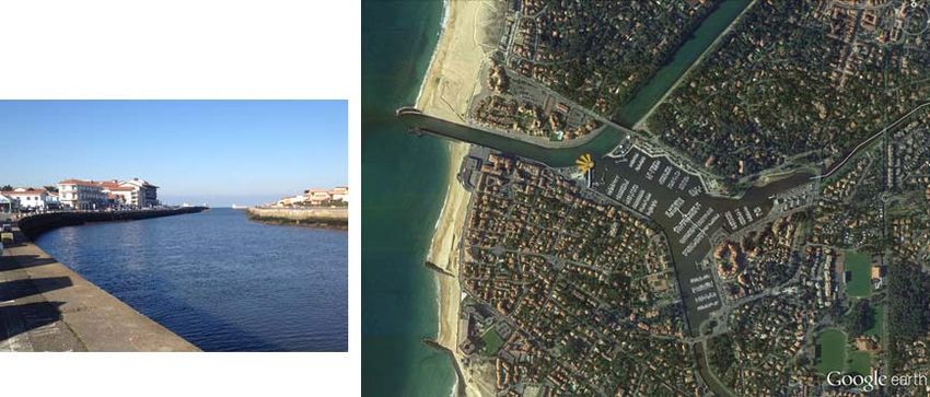
4.5.1 Purpose of the example
The purpose of this example is to simulate the coastal flooding during a storm
event in the town of Capbreton, France, situated on the Atlantic coast
(Figure 4.18).
MIKE 3 Wave Model FM is used to calculate the overtopping rates in the
entrance channel during this event.
Figure 4.18 Left panel shows a picture of the entrance channel, taken from the yel-
low marker on the right panel. Right panel shows a satellite picture of
the city of Capbreton (Source: Google Earth).
32 MIKE 3 Wave Model FM - © DHI A/SCoastal Flooding in Capbreton
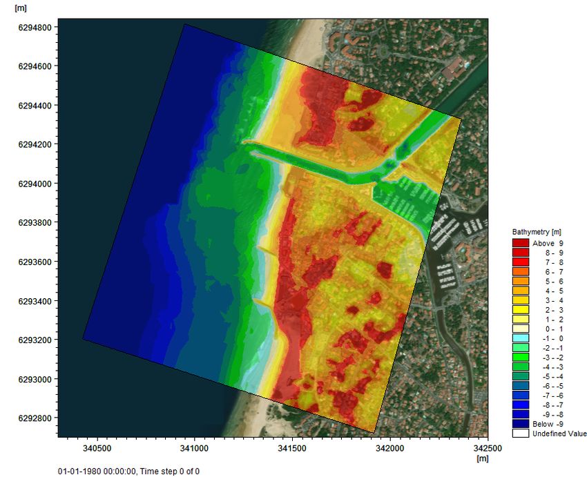
4.5.2 Model setup
The domain covers the entrance channel as well as the coastal areas south
of the port (see Figure 4.2). The model size is 1600m by 1700m. Land is
included as part of the bathymetry to allow coastal flooding in the model. Sim-
ulations are performed using a mesh with more than 100.000 uniform quadri-
lateral elements with a grid spacing of 5m.
The orientation of the domain area is defined to align the model grids with the
entrance channel walls. This orientation is also adapted to the main direction
of the incoming waves.
A wave generation line is located along the 10m depth contour (relative to
NGF: general levelling of France). The simulated event corresponds to the
peak of the main recent and widely documented storm on this coast: storm
Christine, which happened from 2nd to 4th March 2014.
In front of the entrance channel, the peak of the storm is characterised by a
significant wave height of Hm0 = 2.55m, a spectral peak period of Tp = 18.3s,
and a main wave direction of MWD = 290°N. The associated water level is
2.68m NGF. The water level is changed by specifying the initial surface eleva-
tion using a 2D input file, where the surface elevation is 2.68 m. The waves
are irregular, and generated based on a mean JONSWAP spectrum. A wave
absorbing sponge layer is applied along the southern boundary to absorb the
waves going out of the model area. Sponge layers are also placed at the
north and east boundary to absorb the waves propagating up the river.
Note, that the reference level for the internal generation and the sponge lay-
ers should be set to 2.68m.
Powering Water Decisions 33Examples
Figure 4.19 Domain and bathymetry for Capbreton harbour
The Capbreton example runs for about 30 minutes using a 3.2 GHz PC with
16 cores, to simulate 10 minutes (MPI parallelisation with 16 subdomains).
4.5.3 Model results
Figure 4.20 shows a 2D visualisation of the simulated instantaneous surface
elevation at the moment of the arrival of the first generated waves in the
entrance channel. You can make a similar plot using the file Area.plc after
model execution.
34 MIKE 3 Wave Model FM - © DHI A/SCoastal Flooding in Capbreton
Figure 4.20 Model result: 2D visualisation of the instantaneous surface elevation
after 10 minutes.
Figure 4.21 shows a 3D visualisation of the simulated instantaneous surface
elevation. Flooding due to wave overtopping is seen both on the northern and
southern quays of the channel. A screen shot of a video taken from the south-
ern quay during the storm is also presented.
Powering Water Decisions 35Examples
Figure 4.21 Wave overtopping in Capbreton harbour. Upper panel shows a 3D pic-
ture of the simulated instantaneous surface elevation in Capbreton
entrance channel. Lower panel shows a screenshot of a video taken
during the storm on the southern quay of the entrance channel
(Source: YouTube, Mars 2014, retrieved from http://www.you-
tube.com/watch?v=6YuNtXfUHMM)
36 MIKE 3 Wave Model FM - © DHI A/SCoastal Flooding in Capbreton
The wave overtopping in the entrance channel is calculated using discharge
output lines along the vertical walls of the channel. Figure 4.22 shows the
time series of the accumulated discharge across the two output lines, located
on the map. You can make a similar plot using the file Results.plc after model
execution. The discharge is positive when the flow occurs towards land. The
estimated overtopping discharges across the quays can then be used as
inputs for sources in a MIKE FLOOD model of Capbreton combining the
effects of wave overtopping, tide, and of the two rivers flowing into the port.
Figure 4.22 Upper panel shows a "zoomed-in" view of Figure 4.20 in the entrance
channel with the location of two discharge output lines along the quays.
Lower panel shows time series of the accumulated discharges across
these lines over the duration of the simulation.
Powering Water Decisions 37Examples
4.5.4 List of data and specification files
The following data files (included in the \Capbreton folder) are supplied with
MIKE 3 Wave Model FM:
File name: Capbreton.mesh
Description: Mesh file including mesh and bathymetry
File name: Capbreton.m3wfm
Description: MIKE 3 Wave Model FM specification file
File name: Area.plc
Description: Plot Composer file for visualisation of the simulated instantane-
ous surface elevation in the entire domain
File name: Results.plc
Description: Plot Composer file for visualisation of the simulated instantane-
ous surface elevation in the entrance channel and two time series of accumu-
lated discharges
File name: Capbreton.jpg+Capbreton.jpgw
Description: Georeferenced background satellite image file
38 MIKE 3 Wave Model FM - © DHI A/SDomain
5 BASIC PARAMETERS
5.1 Domain
Providing MIKE 3 Wave Model FM with a suitable mesh is essential for
obtaining reliable results from your model. Setting up the mesh includes
selection of the appropriate area to be modelled, adequate resolution of the
bathymetry, wave and flow fields under consideration and definition of codes
for porosity zones, sponge layers and closed boundaries. Furthermore, the
resolution in the geographical space must also be selected with respect to
stability considerations.
MIKE 3 Wave Model FM is based on the flexible mesh approach. A layered
mesh is used: In the horizontal domain an unstructured mesh is used while in
the vertical domain a structured mesh is used (see Figure 5.1). The vertical
mesh is based on either sigma-coordinates or combined sigma/z-level coor-
dinates. For the hybrid sigma/z-level mesh sigma coordinates are used from
the free surface to a specified depth and z-level coordinates are used below.
The different types of vertical mesh are illustrated in Figure 5.2. The elements
in the sigma domain and the z-level domain can be prisms or bricks (hexahe-
drals) whose horizontal faces are triangles and quadrilateral elements,
respectively. The elements are perfectly vertical and all layers have identical
topology.
Figure 5.1 3D mesh using sigma coordinates
Powering Water Decisions 39BASIC PARAMETERS
Figure 5.2 Illustrations of the different vertical grids.
Upper: sigma mesh, Lower: combined sigma/z-level mesh with simple
bathymetry adjustment. The red line shows the interface between the z-
level domain and the sigma-level domain.
5.1.1 Mesh and bathymetry
The mesh and bathymetry can be specified either using a mesh file or a
bathymetry data file.
Mesh file
You generate your mesh file in the MIKE Zero Mesh Generator, which is a
tool for the generation and handling of unstructured meshes, including the
definition and editing of boundaries.
The mesh file is an ASCII file including information of the map projection and
of the geographical position and bathymetry (Bed elevation) for each node
point in the mesh. The file also includes information of the node-connectivity
in the mesh.
40 MIKE 3 Wave Model FM - © DHI A/SDomain
Bathymetry data file
You generate your bathymetry data file in the MIKE Zero Bathymetry Editor,
which is a tool for the generation of structured meshes. An example with a
step-by-step description of how to use the Bathymetry Editor for creating a
bathymetry data file is included with the installation. Please find this example
in your installation folder under Examples\MIKEZero\BatEdit.
The bathymetry data file is a dfs2 file which contains the bathymetry (Bed ele-
vation) and the following geographical information of the computational
domain
The map projection
The geographical position of the grid origin
The grid orientation.
The grid orientation is defined as the angle between true north and the y-axis
of the model measured clockwise. A mnemonic way of remembering this defi-
nition is by thinking of NYC, which normally means New York City, but which
for our purpose means "from North to the Y-axis Clockwise", see Figure 5.3.
Figure 5.3 Definition of model orientation
The bathymetry data file also contains information of the true land value. True
land value is the minimum value you have specified for land points when you
prepared the bathymetry. All grid points with a depth value equal to or greater
than the value you specify will be excluded from the computational domain.
The value representing land is the forth element in the custom block called
M21_Misc which consists of 7 elements of type float. The computational
mesh is shown in the graphical view.
The bathymetry data file does not contain any information of the boundaries.
Therefore starting at the grid origin and going counter-clockwise a boundary
code (2, 3, 4 …) is set for each open boundary section of the grid. The bound-
ary codes can be seen by clicking on the graphical view and select "Show
mesh".
The bathymetry data file can also be converted to a mesh file using the MIKE
Zero Mesh Converter Tool. This will allow you to edit the boundary codes
using the MIKE Zero Data Viewer. Note, that a simulation using a mesh file
will give different result than using the bathymetry data file directly due to the
Powering Water Decisions 41BASIC PARAMETERS
difference in the determination of the bed elevation in the cell center (see Bed
elevation).
Bed elevation
Using a mesh file for specification of the mesh and bathymetry, the bed eleva-
tion is given at the nodes (vertices) of the elements. The governing equations
are solved using a cell-centred finite volume approach. Here the bed level is
required at the cell center. This bed level is determined as the mean value of
the node values.
Using a bathymetry data file for specification of the mesh and bathymetry, the
bed elevation at the cell center of the elements is determined as the bed ele-
vation specified in the input data file. The bed elevation at the nodes is deter-
mined as the area-weighted mean values of the bed elevation in the elements
connected to the node and the weight factors are the areas of the connected
elements.
5.1.2 Domain specification
Map projection
When the mesh is specified using a mesh file generated by the MIKE Zero
Mesh Generator or the mesh is specified using a bathymetry data file gener-
ated by the MIKE Zero Bathymetry Editor the map projection is defined in the
input data file and is only shown for reference in the user interface. If the map
projection is not defined in the mesh file, you have to select the correct map
projection corresponding to the data in the mesh file.
Minimum depth cutoff
If the bathymetry level in an element is above the minimum depth cutoff value
then the minimum depth cutoff value is replacing the actual bathymetry value
in the computations. Please note that the minimum depth cutoff value may be
negative as the bathymetry levels is often so in the mesh file.
If you also apply a Datum shift - the depth cutoff is relative to the corrected
depths.
For instance - you have a mesh file with values between +2 and -20 meters.
You then shift these to a different datum with a shift of +1 meters. Your cor-
rected bathymetry now ranges between +1 and -21 m. You can then cutoff all
depths above -2m, leaving the bathymetry used in the model to range
between -2 and -21 m.
Datum shift
You can use any convenient datum for setting up the mesh of your model.
This can be Chart Datum (CD), Lowest Astronomical Tide (LAT) or Mean Sea
Level (MSL). The actual datum is unimportant.
42 MIKE 3 Wave Model FM - © DHI A/SDomain
What is important, however, is that for each simulation you must provide the
model with the correct height of the model reference level relative to the
datum used in the setup of your bathymetry. Specifying the datum shift does
this. In this way it is possible to carry out simulations using a range of different
water levels without having to alter the mesh file.
If you do not plan to apply different water levels in different simulations it is
recommended that you set up your bathymetry with the datum that you plan
use in the simulations, thus having a datum shift of 0 m.
Note: A datum shift of e.g. 2 m (-2 m) means the water depth is increased
(decreased) by 2 m in all node points.
Mesh decomposition
To improve the performance of the numerical scheme it is possible to include
reordering of the mesh (renumbering of the element and node numbers). This
can significantly speed up the computational time by optimizing the memory
access.
To improve the performance of the numerical scheme a domain decomposi-
tion technique is applied. If reordering is included the reordering is applied at
subdomain level.
Note: When reordering is applied the numbering of the nodes and elements
in the output files has been changed compared to the information in the mesh
file. The information in the log file corresponds to the new ordering.
5.1.3 Vertical mesh
In the vertical domain a layered mesh is applied. Two different types of the
mesh can be used:
Sigma
Combined sigma/z-level
In most wave applications it is recommended to use sigma coordinates for
the vertical discretization. The advantage using sigma coordinates is their
ability to accurately represent the bathymetry and provide consistent resolu-
tion near the bed.
The recommended number of vertical layers depends on the model. A rough
guideline is 4-7 layers for modelling surface elevation, and 8-12 layers for
modelling breaking waves.
Sigma
In the sigma domain the vertical distribution of the layers can be specified in
three different ways:
Powering Water Decisions 43BASIC PARAMETERS
Equidistant
Layer thickness
Variable
Figure 5.4 Examples of vertical distribution of layers for a water column 100 m
deep. A number of 12 layers has been applied for all three options.
Left column: Equidistant distribution
Middle column: Layer thickness distribution
Right column: Variable distribution
For all three options you must specify the number of vertical layers (ele-
ments).
Selecting equidistant distribution, the layers are distributed equidistant across
the water depth.
Selecting layer thickness distribution, the fraction of each layer’s thickness
across the water depth must be specified. Note that the sum of the values for
the layer thickness must be equal to 1.
Selecting variable distribution, you must specify three vertical distribution
parameters:
1. sigma_c (c )
c is a weighting factor between the equidistant distribution and the
stretch distribution. The range is 0 c 1 . The value 1 corresponds to
equidistant distribution and 0 corresponds to stretched distribution.
A small value of c can result in linear instability.
2. theta ( )
is the surface control parameter. The range is 0 20 .
44 MIKE 3 Wave Model FM - © DHI A/SDomain
3. b is the bottom control parameter. The range is 0 b 1 .
The variable s-coordinates are obtained using a discrete formulation of the
general vertical coordinate (s-coordinate) system proposed by Song and
Haidvogel (1994).
If BASIC PARAMETERS
Figure 5.6 Example of vertical distribution using variable distribution. Number of
layers: 10, sigma_c = 0.1, theta = 5, b = 1
Combined sigma/z-level
For the combined sigma/z-level mesh sigma coordinates are used from the
free surface to a user specified level (sigma depth) and below that z-level
coordinates are used.
Figure 5.7 Example of vertical distribution using combined sigma/z-level
When flood and dry is included in the simulation, the flooding and drying (see
p. 53) is restricted to areas within the sigma domain. Therefore the sigma
depth must be selected so that the minimum water level during the simulation
does not become lower than that sigma depth.
The specification of the mesh in the sigma domain is done as described in the
previous section (see p. 43). In the z-level domain the vertical distribution of
the layers can be specified in two different ways:
46 MIKE 3 Wave Model FM - © DHI A/SDomain
Equidistant
Layer thickness
For both options you must specify the number of vertical layers (elements)
and the sigma depth.
Selecting Equidistant distribution the constant layer thickness must be speci-
fied.
Selecting Layer thickness distribution the thickness of each layer must be
specified. Layer 1 correspond to the bottom layer, layer 2 corresponds to the
second layer from the bottom and so on.
The type of bathymetry adjustment can be specified in two ways:
Simple adjustment
Advanced adjustment
When selecting simple adjustment, the bottom depth is rounded to the near-
est depth except when the bottom depth is below the minimum z-level. Here
a bottom fitted approach is applied to take into account the correct depth.
When selecting advanced adjustment, a bottom fitted approach is applied in
the whole z-level domain which allows the correct depth to be taken into
account. Using the advanced adjustment you must also specify a minimum
layer thickness. Normally, it can be specified as 1/100 of the constant layer
thickness when the option Equidistant distribution is selected and corre-
spondingly 1/100 of the minimum layer thickness when the option Layer
thickness distribution is selected.
Depth correction
When combined sigma/z-level mesh is applied for the vertical discretization
the correction bathymetry is limited. If “Simple adjustment” is selected for the
bathymetry adjustment, depth correction and morphological changes due to
sediment transport are not allowed. If “Advanced adjustment” is selected for
the bathymetry adjustment only small corrections of the bathymetry are pos-
sible. The correction factor for the layer thickness is not allowed to be less
than zero or larger than one except for the bottom cell.
A detailed description of the bottom fitted approach can be found in the scien-
tific documentation for MIKE 21 & MIKE 3 Flow Model FM, Hydrodynamic
and Transport Module.
Note: Although a bottom fitted approach can be applied in which the correct
depth is taken into account, the flow at the bottom still needs to pass obsta-
cles either sidewards or upwards whenever encountered. Therefore smooth-
ing of bathymetry may improve the results.
Powering Water Decisions 47BASIC PARAMETERS
5.1.4 Boundary names
When the mesh is specified using a mesh file generated by the MIKE Zero
Mesh Generator you already have defined a code value for porosity zones
and sponge layers.
Figure 5.8 shows the definition of codes in a simple application. In this case 2
boundary codes have been detected from the mesh file specified in the
domain parameters; code 2 and code 3. Code 1 is interpreted as closed land
boundaries.
Figure 5.8 The definition of boundary codes in a mesh is made in the Mesh Gener-
ator
When the mesh is specified using a bathymetry data file generated by the
MIKE Zero Bathymetry Editor the boundary code is defined as described on
the Domain dialog.
In the main Boundary names dialog you can re-name the code values to
more appropriate names, see Figure 5.9.
Figure 5.9 Change of default boundary code names to more appropriate names
5.2 Time
The period to be covered by the simulation is specified in this dialog. You
have to specify the simulation start date, the overall number of time steps and
the overall time step interval. The overall discrete time steps specified on this
page are used to determine the frequency for which output can be obtained.
48 MIKE 3 Wave Model FM - © DHI A/SYou can also read