Modeling Imprecision in Perception, Valuation and Choice
←
→
Page content transcription
If your browser does not render page correctly, please read the page content below
Modeling Imprecision in
                 Perception, Valuation and Choice∗
                                   Michael Woodford
                                  Columbia University
                                  September 15, 2019

                                           Abstract
           Traditional decision theory assumes that people respond to the exact fea-
       tures of the options available to them, but observed behavior seems much less
       precise. This review considers ways of introducing imprecision into models of
       economic decision making, and stresses the usefulness of analogies with the
       way that imprecise perceptual judgments are modeled in psychophysics — the
       branch of experimental psychology concerned with the quantitative relationship
       between objective features of an observer’s environment and elicited reports
       about their subjective appearance. It reviews key ideas from psychophysics,
       provides examples of the kinds of data that motivate them, and proposes lessons
       for economic modeling. Applications include stochastic choice, choice under
       risk, decoy effects in marketing, global game models of strategic interaction,
       and delayed adjustment of prices in response to monetary disturbances.

   ∗
    Prepared for the Annual Review of Economics, volume 12. I would like to thank Rava Azeredo da
Silveira, Andrew Caplin, Paul Glimcher, Mel Win Khaw, Ziang Li, Stephen Morris, Rafael Polania,
Arthur Prat-Carrabin, Antonio Rangel, and Christian Ruff for helpful discussions.
Economic analysis seeks to explain human behavior in terms of the incentives that
people’s situations provide for taking various actions. It is common to assume that
behavior responds to the objective incentives provided by the situation. However, it
is evident that people can only respond to incentives (the quality of goods on offer,
their prices, and so on) to the extent that they are correctly perceived; and it is
not realistic to assume that people (as finite beings) are capable of perfectly precise
discrimination between different objective situations. Thus people should not be
modeled as behaving differently in situations that they do not recognize as different,
even if it would be better for them if they could.1
But how should imprecision in people’s recognition of their true situations be
introduced into economic models? This review will argue that economists have much
to learn from studies of imprecision in people’s perception of sensory magnitudes.
The branch of psychology known as psychophysics has for more than 150 years sought
to carefully measure and mathematically model the relationship between objective
physical properties of a person’s environment and the way these are subjectively
perceived (as indicated by an experimental subject’s overt responses, most often, but
sometimes by physiological evidence as well). Here we review some of the key findings
from this literature, and suggest possible lessons for economic modeling.2
While the phenomenology of sensory perception is quite rich, we stress here the
power of a single modeling approach to explain many well-known findings. In this
approach, imprecision in the judgments that subjects express is attributed to impre-
cision in the way that the objective external situation is represented by a pattern
of activity within the subject’s nervous system; the responses can be modeled as
optimal, subject to the constraint that the response rule must be based on the im-
precise internal representation. We propose that this same approach might usefully
be adopted in economic modeling, and provide some examples of its application.
Section 1 reviews the classic problem (first studied by Ernst Weber in the 1830s)
of judgments about the comparative magnitude of two stimuli along some dimension,
and discusses the applicability of similar models to the problem of stochastic choice.
Section 2 then considers more complex experimental designs in which the magni-
tude of a single stimulus is estimated, choosing from among a continuum of possible
responses; this is of particular interest as an element in decisions that require advan-
tages and disadvantages to be traded off against one another. It is argued that the
1
See Luce (1956) and Rubinstein (1988) for early discussions of this issue.
2
For alternative discussions of possible lessons for economics, see Weber (2004) or Caplin (2012).
1estimation biases that are observed in sensory contexts provide a potential explana-
tion for patterns of choice behavior that are instead often attributed to non-standard
preferences. And finally, section 3 discusses ways in which judgments about a given
sensory magnitude can be influenced by the context in which it appears; it is proposed
that similar mechanisms can explain choice behavior that appears inconsistent with
the existence of any coherent preference ordering.
1 The Stochasticity of Comparative Judgments
A first important lesson of the psychophysics literature is that not only are people
(or other organisms) unable to make completely accurate comparisons as to which is
greater of two sensory magnitudes — which of two weights is heavier, which of two
lights is brighter, etc. — when the two magnitudes are not too different, but that the
responses given generally appear to be a random function of the objective properties
of the two stimuli that are presented. At the same time, the random responses
of experimental subjects are not “pure noise” — that is, completely uninformative
about the truth. Thus rather than it being the case that any two stimuli either can
be told apart (so that the heavier of two weights is always judged to be heavier,
whenever those two weights are presented for comparison), or cannot be (so that the
subject is equally likely to guess that either of the weights is the heavier of the two),
what one typically observes is that the probability of a given response (“the second
weight seems heavier”) increases monotonically with increases in the actual relative
magnitude of the two stimuli. Experimental procedures often focus on the estimation
of this increasing functional relationship, plotted as a “psychometric function.”3
Figure 1 provides an example of such plots (from Krueger, 1984), when the stim-
ulus feature is numerosity, the number of items in a disordered array (in this case, Xs
typed on a sheet of paper); in the experiment, a subject is asked to judge whether a
second array is more or less numerous than a first (reference) array, on the basis of
a quick impression (rather than counting). While this is not one of the most classic
examples,4 it has the advantage (for purposes of this review) of shedding light on the
3
See, e.g., Gescheider (1997, chap. 3), Glimcher (2011, chap. 4), or Kingdom and Prins (2010,
chap. 4).
4
In particular, for many standard examples, the stimulus feature that is compared — such as
weight, length, brightness, speed, or direction of motion — is one that takes a continuum of possible
2-' ~, series being followed by a downturn at the upper end
.6 .8 1.0 1.2 of the series (see his Figure 3).
Exponent
Discrimination
Figure 4. Magnitude estimation: Distribntion of exponents for The mean and SD of the percentage of errors was
individual subjects. The dotted Hnedepicts a normal distribution.
31.71010 ± 7.44010. Errors decreased significantly from
ponent for subjects in the lower range, but decreasing
90
it for those in the upper range (see Figure 4). Greater I
practice alone did not reduce the variability in the
+ 1.0 a 25 Xs
I
: _~ •.--
•.«:
postcue condition, because variability was stable + .5 70
I • .--
within each condition (SOs of the exponent were .148 o ---------::.+",.. ::---------- 50
and .143 for the precue replications and .088 and
-.5
•.---e I
.090 for the postcue replications). The SOs within •.'--- I 30
each condition did not differ significantly (t < 1 in -;;;- -1 .0 /'./ i
1
all cases), whereas those compared between condi- ~ l : - - - - - - - j - - - - - - - - - - - I 10
tion did (P < .001 in all cases). ~+1.0 b.l00 Xs I
- -;
Feedback did not eliminate all intersubject vari- ~ +.5
I
I !t.--.--'. 70-:
ability, though, because the postcue replications cor- Q)
o --------~-~------------ 50 C
: .»• • , ••
related moderately on both the scale factor (+ .54) ~
o
.-'. I
and the exponent (+.61). These correlations are nearly -.5 .,._.-•.• -~ I 30 -g
as large as the corresponding ones in the precue con- ..- I
Q)
dition ( + .69 and +.79). Furthermore, the precue and I ~
":>
postcue conditions correlated on the scale factor c 400 Xs I
( + .49) and on the exponent ( + .50), which again in-
+1.0
i e'-'-
+ .5 I e·- . 70
dicates that feedback did not eliminate all consistent I It---- •
intersubject differences. (In every case, df =98 and o ------;~~;;o-:--------- 50
1.·--
p < .001.) -.5 I
••••• .>
30
If only intrasubject variability was present, then .---;
I
I
the group SOs at particular stimulus sizes (solid ver: -1.0
I
tical lines in Figure 3) would be only 71010 (1/V2)
of the intrasubject SOs (dotted vertical lines in Fig- -4 -2 o +2 +4
Deviation (steps) from standard
ure 3). This was approximately true in the postcue
condition (65070), but not in the precue condition Figure 5. Discrimination: Proportion of comparison stimuli
Figure 1:
(81010), in which greater intersubject Psychometric
variability would Judged functions for comparisons
larger than standard stimuH (scaled as z scores of onnumerosity.
left side The number of
be expected. and as percent scores on right side), by size of standard and size
items increased,
in the reference of deviation of comparison
100, orstimulus 400 from standard. Step·
(a),sizes
As the number of Xs present the group array is 25, in panels
were 1, 3, and 9, respectinly, for standards of 15, 100, and 400.
(b), and (c) respectively.
SOs generally increased in(Reproduced
the precue condition (slope Thus,
from Krueger, 1984.) the range of deviations in number of Xs was -4 to +4, -12
of .08), but not in the postcue condition (slope of to +12, and -36 to +36, respectiveiy.
imprecise mental representation of numerical information — and thus of offering an
especially plausible analogy for judgments of economic value.
In each panel of the figure, the number n1 of items in the reference array is
fixed, and the fraction of trials on which subjects judge the second array to be more
numerous is plotted as a function of the true difference in numerosity n2 − n1 ;5 the
value of n1 increases from 25 to 100 to 400 as one proceeds from the top panel to the
bottom. In each panel, the probability of judging n2 to be larger than n1 is steadily
increasing as a function of the true difference.
A classic approach to modeling imprecise comparisons of this kind, dating to the
work of Fechner (1860), supposes that a true stimulus magnitude x gives rise to an
internal representation r, drawn from a probability distribution p(r|x) that depends
values, so that one can meaningfully speak of response probabilities as varying continuously with
the true stimulus magnitude.
5
This difference is reported in “steps.” A “one step” increase means one more X in the top panel,
three more in the middle panel, and nine more in the bottom panel.
3on the true magnitude. This representation r can be understood to refer to a pattern
of neural activation, in regions of the cortex involved in processing stimuli of that kind,
as a result of the person’s (or other organism’s) contact with a stimulus of magnitude
x; it is random because of randomness in the way that neurons fire in response to the
signals that they receive. A comparative judgment between two magnitudes x1 and
x2 is made on the basis of the corresponding internal representations r1 and r2 ; the
randomness of r1 and r2 makes such comparisons random, even if the rule by which
responses are generated is optimal subject to the constraint that it must be based on
the noisy internal representations.
To make this more concrete, a widely used model due to Thurstone (1927) assumes
that the internal representation can be summarized by a single real number, and that
it is drawn from a normal distribution N (m(x), ν 2 ), where m(x) is an increasing
function of the true magnitude, and the standard deviation ν > 0 is independent of
the true magnitude.6 If for each of two stimuli x1 and x2 , the internal representation ri
is an independent draw from the corresponding distribution, then an optimal decision
rule will judge that x2 seems greater than x1 if and only if r2 > r1 .7 This in turn
implies that the probability of such a judgment, conditional on the true magnitudes
x1 and x2 (known to the experimenter) is predicted to be
m(x2 ) − m(x1 )
Prob[“x2 greater”|x1 , x2 ] = Φ √ , (1.1)
2ν
where Φ(z) is the CDF of a standard normal distribution. Thus the probability
of correctly distinguishing the relative magnitudes of two stimuli depends on their
distance |m(x2 ) − m(x1 )| from one another on the “Thurstone scale” established by
the mapping m(x).8
This equation predicts the shape of a psychometric function, if one plots the
response probability as a function of x2 for some fixed value of x1 . If the measured
6
This is Thurstone’s celebrated “Case V.”
7
Here we assume a “two-alternative forced choice” experimental design, in which the subject must
select one of the two possible responses, regardless of their degree of confidence in their answer. If
the prior distribution from which true values (x1 , x2 ) are drawn is symmetric ((x2 , x1 ) has exactly
the same probability of being presented as (x1 , x2 )), then this is the response rule that maximizes
the probability of a correct choice.
8
Data on the frequency with which different comparative judgments are made, such as that
plotted in Figure 1, can allow the identification of this scale up to an affine transformation.
4response probabilities are z-transformed,9 equation (1.1) implies that one should have
m(x2 ) − m(x1 ) m0 (x1 )
z(Prob) = √ ≈ √ · (x2 − x1 ), (1.2)
2ν 2ν
for values of x2 sufficient close to the reference magnitude x1 . Thus when the rela-
tionship is plotted as in Figure 1,10 the relationship should be approximately linear,
as shown in the figure — with a response probability of 0.5 when x2 − x1 = 0, and a
slope proportional to m0 (x), evaluated at the reference magnitude.
The figure not only shows that the psychometric function in each case is roughly
of the predicted form (1.2), but allows m0 (x) to be evaluated at three different points
in the range of possible stimuli. One finds that the size of the difference in number
required for a given size of effect on the response probability is not independent of the
range of numerosities being compared. Suppose that one defines the “discrimination
threshold” as the average of the increase in the number of Xs required for the proba-
bility of judging n2 to be greater than n1 to rise from 0.5 to 0.75, and the decrease in
number required for this probability to fall from 0.5 to 0.25. Then in the data shown
in Figure 1, this threshold is found to be 3.1 when n1 = 25, but 11.7 when n1 = 100,
and 32.3 when n1 = 400.
This increase in the discrimination threshold as the reference stimulus magnitude
increases is called “diminishing sensitivity,” and is an ubiquitous finding in the case
of extensive quantities such as length, area, weight, brightness, loudness, etc. This is
consistent with the Thurstone model, under the assumption that m(x) is a strictly
concave function. A famous formulation, “Weber’s Law,” asserts that the discrimi-
nation threshold should increase in proportion to the reference magnitude n1 ; as first
proposed by Fechner (1860), this would follow from the model in the case that one
assumes that m(x) is (some affine transformation of) the logarithm of x.11
9
That is, the probabilities are replaced by z(p) ≡ Φ−1 (p), the inverse of the function p = Φ(z).
10
Note that in each of the panels of the figure, the vertical axis is linear in the “z score” z(p)
rather than in the probability p (marked on the right-hand side of the panel)
11
Even when Weber’s Law holds approximately, it is often only for variation in the stimulus
magnitude over some range, beyond which the approximation breaks down. See, for example, the
plots of how discrimination thresholds vary with stimulus magnitude in a variety of sensory domains
in Ganguli and Simoncelli (2016). Weber’s Law has sometimes been asserted also to hold for the
perception of numerosity (e.g., Nieder and Miller, 2003; Dehaene, 2003; Cantlon and Brannon, 2006),
but the evidence is much stronger for diminishing sensitivity at a rate that is not necessarily precisely
consistent with Weber’s Law. In the estimates from Krueger (1984) cited above, the discrimination
51.1 Encoding and Decoding as Distinct Processes
In the early psychophysics literature, the randomness of comparisons of the kind dis-
cussed above was often modeled by simply postulating that an objective stimulus
magnitude x gave rise to a perceived magnitude x̂, drawn randomly from a distribu-
tion that depended on x. The probability of an incorrect comparison then depended
on the degree of overlap between the distributions of possible perceived values asso-
ciated with different but similar true magnitudes, as in the discussion above.
Here we have instead taken a more modern point of view, in which decisions are
based on a noisy internal representation r, which is not itself a perceived value of
the magnitude x, but only an available piece of evidence on the basis of which the
brain might produce a judgment about the stimulus, or a decision of some other kind.
(Note that r need not be measured in the same units as x, or even have the same
dimension as x.) The cognitive process through which judgments are generated is
then modeled as involving (at least) two stages: encoding of the stimulus features (the
process through which the internal representation is produced), followed by decoding
of the internal representation, to draw a conclusion about the stimulus that can be
consciously experienced and reported.12
In this way of conceiving matters, perception has the structure of an inference
problem — even though the “decoding” process is understood to occur automatically,
rather than through conscious reasoning — and tools from statistical decision theory
have proven useful as a source of hypotheses. In particular, once matters are conceived
in this way, it is natural to consider (at least as a theoretical benchmark) models in
which the decoding is assumed to represent an optimal inference from the evidence
provided by the internal representation.13
Why should one wish to complicate one’s model of imprecise comparisons in this
way, rather than simply directly postulating a distribution of perceived values, about
which an experimental subject might then be interrogated? One answer is that the
development of constantly improving methods of measurement of neural activity has
made the concept of an internal representation, distinct from the observable behavior
threshold increases with the reference numerosity with an elasticity that is instead about 0.85.
12
Dayan and Abbott (2001, chap. 3) provide a textbook discussion.
13
Our explanation above of why it makes sense to assume that the judgment “x2 seems greater”
is produced if and only if r2 > r1 is an example of such an assumption of optimal decoding; see
footnote 7.
6that may be based on it, something more than just a latent variable that is postulated
for convenience in explaining the logical structure of one’s model of the observables;
if one wishes to use such measurements to discipline models of perception, then the
candidate models must include variables to which the neural measurements may be
taken to correspond.14
But another important answer is that such a theory allows one to understand in
a parsimonious way how changes in the context in which a stimulus is presented can
affect the perceptual judgments that are made about it. In a binary-comparison task
of the kind discussed above, the probability of a subject giving a particular response is
not a function solely of the objective characteristics of the two stimuli presented; it can
also depend, for example, on the frequency with which the second stimulus magnitude
is greater than the first, rather than the reverse,15 or on the relative incentive for a
correct response in the two possible cases. It is easy to understand how these latter
considerations can influence a subject’s judgments in the encoding/decoding model:
even if one supposes that in the encoding stage, the distribution from which the
representation r is drawn depends only on the particular stimulus feature x, and not
on any other aspects of the context,16 an optimal decoding rule should take other
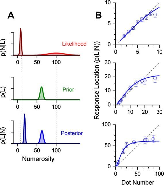
aspects of the context into account. In particular, from the standpoint of Bayesian
decision theory, the optimal inference to make from any given evidence depends on
both the decision maker’s prior and on the objective (or reward) function that he/she
seeks to maximize.
Signal detection theory (Green and Swets, 1966) applies this kind of reasoning to
the analysis of perceptual judgments. Figure 2 (which reproduces Figures 4-1 and
4-2 from Green and Swets) shows a classic application of the theory. The figure plots
data from a single subject, in an experiment in which on each trial one of two auditory
stimuli (denoted s and n) are presented, and the subject’s task is to indicate which
14
See Dayan and Abbott (2001, chap. 3) for examples.
15
It was assumed above, in our discussion of the normative basis for a particular rule for de-
termining the perceptual judgment (footnote 7), that either stimulus was equally likely to be the
greater one, and this is true in many experiments. But it is possible for the frequencies to differ in
a particular experiment (or block of trials), and for subjects to learn this (or be told), as illustrated
below.
16
This is a common simplifying assumption, but in fact context can influence encoding as well, as
discussed in section 3.
7Figure 2: Conditional response probabilities in a signal detection task. The tradeoff
is shown between the “hit rate” (vertical axis) and “false alarm rate” (horizontal
axis), as one varies the prior probability of occurrence of the two stimuli (left panel),
or the relative rewards for correct identification of the two stimuli (right panel). In
each case, the efficient frontier (“ROC curve”) is shown by the bowed solid curve.
(Reproduced from Green and Swets, 1966.)
is the case (making one of the two possible responses, S or N ).17 In each of several
blocks of trials, the same two stimuli are used (the stimulus presented on each trial is
always either s or n), but the prior probability of s rather than n being presented may
vary across blocks, as may the financial incentive given the subject to avoid “Type
I” as opposed to “Type II” errors. Each of the circles in the figure plots the subject’s
conditional response probabilities for one block of trials.
The location of each circle indicates both the subject’s “hit rate” P (S|s) (the
probability of correctly detecting the signal, when it is present), on the vertical axis,
and the subject’s “false alarm rate” P (S|n) (the probability of incorrectly reporting a
signal when none is present), on the horizontal axis. The diagonal line in each figure
indicates the combinations of hit rate and false alarm rate that would be possible
under pure chance (that is, if the subject were entirely deaf); all points above the
17
The stimulus s is one in which a signal (a tone) is presented, amid static, while stimulus n
consists only of the noise. The experiments developed out of work (originally with visual stimuli)
seeking to measure the accuracy of human operators of radar equipment (Creelman, 2015).
8diagonal indicate some ability to discriminate between the two stimuli, with perfect
performance corresponding to the upper left corner of the figure.
If one supposes that a subject should have a perception S or N that is drawn from
a probability distribution that varies depending on whether the stimulus presented
is s or n — but that depends only on the stimulus presented and not other aspects
of the context — then one should expect a given subject to exhibit the same hit rate
and false alarm rate in each block of trials. (Of course one could expect to see small
differences owing to random sampling error, given the finite length of each block of
trials, or perhaps drift over time in the subject’s functioning owing to factors such
as fatigue — but these differences should not be systematically related to the prior
frequencies or to incentives.)
Instead, in the figure one sees systematic effects of both aspects of the context.
In the left panel, the reward is the same for correct identification of either stimulus,
but the probability of presenting stimulus s on any given trial varies across the blocks
of trials (it is 0.1, 0.3, 0.5, 0.7 or 0.9, depending on the block); and one sees that as
the prior probability of the state being s is increased, both P (S|s) and P (S|n) are
monotonically increasing. In the right panel, both stimuli are presented with equal
probability, but the relative incentive for correct identification of the two cases is
varied; and one sees that as the relative reward for correct recognition of state s is
increased, both P (S|s) and P (S|n) are again monotonically increasing.
Both phenomena are easily explained by a model that distinguishes between the
noisy internal representation r upon which the subject’s response on any trial must
be based, and the subject’s classification of the situation (by giving response S or
N ). Suppose, as in the model above, that r is a single real number,18 and that it is
drawn from a Gaussian distribution N (µi , ν 2 ), with a variance that is the same for
both stimuli, but a mean that differs depending on the stimulus (i = s or n). Let
us further suppose, without loss of generality, that µs > µn , so that the likelihood
ratio in favor of the stimulus being s rather than n is an increasing function of r. If
the subject’s response on any trial must be based on r alone, an efficient response
criterion — in the sense of minimizing the probability of a type I error subject to
18
In this kind of task, because there are only two possible true situations (s or n), even if the
internal representation were high-dimensional, it clearly suffices to describe it using a single real
number as a sufficient statistic, namely the likelihood ratio of the two hypotheses given the noisy
evidence. See discussion in Green and Swets (1966).
9an upper bound on the probability of type II errors, or vice versa — is necessarily
a likelihood ratio test,19 which in the present case means that the subject should
respond S if and only if r exceeds some threshold c.
Varying the value of c (which corresponds to changing the relative weight placed
on avoiding the two possible types of errors) allows one to generate a one-parameter
family of efficient response rules, each of which implies a particular set of conditional
response probabilities (and hence corresponds to a point in the kind of plots shown in
Figure 2). In the case of a particular value of the ratio (µs − µn )/ν, which determines
the degree of discriminability of the two stimuli given the subject’s noisy encoding
of them, the points corresponding to this family of efficient response rules can be
plotted as a curve, known as the “receiver operating characteristic” or ROC curve.
This is shown as a concave, upward-sloping curve in each of the panels of Figure
2; here the ROC curve is plotted under the assumption that µs and µn differ by 0.85
standard deviations. We see that under this parameterization, the subject’s pattern
of responses falls close to the efficient frontier in all cases. Moreover, the change in the
subject’s response frequencies is in both cases consistent with movement along the
efficient frontier in the direction that would be desirable in response to an increased
reason to prioritize an increased hit rate even at the expense of an increase in the
false alarm rate.
Hence the subject’s response probabilities are easily interpreted as reflecting a
two-stage process, in which encoding and decoding are influenced by separate factors,
which can be experimentally manipulated independently of one another. On the one
hand, an experimenter can change aspects of the stimuli, unrelated to the feature on
the basis of which they are to be classified, that can affect the precision of encoding
(for example, varying the length of time that a subject is able to listen to auditory
stimuli before expressing a judgment); if this changes the value of ν, this should shift
the location of the ROC curve along which the subject should operate (whatever the
prior and incentives may be). And on the other hand, an experimenter can change
the prior and/or incentives, which should affect the relative priority assigned to the
two possible types of error, and hence the location on any given ROC curve where the
subject would ideally operate. The fact that encoding and decoding are determined
by distinct sets of parameters that can be independently manipulated makes it useful
19
This follows from the Neyman-Pearson lemma of statistical decision theory; again see Green
and Swets (1966).
10to model the subject’s judgments as the outcome of two separate processes of encoding
and decoding.20
1.2 Implications for Economic Models
The above review of the way in which imprecise comparisons have been successfully
modeled in sensory domains suggests a number of implications for models of imprecise
economic decisions. For example, some authors propose to introduce cognitive im-
precision into economic models by assuming that agents can respond only to a coarse
classification of the current state of the world, but assume that an agent should know
with certainty to which element of some partition of the state space the current state
belongs.21 In the case of a continuous state space, such a model implies that certain
states that differ only infinitesimally should nonetheless be perfectly distinguished,
because they happen to fall on opposite sides of a category boundary; but nothing
of the sort is ever observed in the case of perceptual judgments. Instead, if one sup-
poses that the imprecision that wants to capture should be analogous to imprecision
in the way that our brains recognize physical properties of the world, then one should
model internal representations as probabilistically related to the external state, but
not necessarily as discrete.
The literature on “global games”22 models imprecise awareness of the state of the
world in a way that is more consistent with what we know about perception. In
models of this kind, the true state is assumed to be a continuous variable, but agents
are not assumed to be able to observe it precisely. This is shown to have important
consequences for the nature of equilibrium, even when the imprecision in individual
agents’ private observations of the state is infinitesimally small (but non-zero). For
example, even in models of bank runs or currency attacks that allow for multiple
equilibria when all agents observe the state with perfect precision, there can be a
unique equilibrium (and hence predictable timing of the run or attack) if decisions
must be based on slightly imprecise private observations.
Here the imprecision in private observations is modeled by assuming that each
agent has access to the value of a signal r, equal to the true value of the state x plus
a random error term which is an independent draw for each agent from some (low-
20
Green and Swets (1966, chap. 4) call this the “separation of sensory and decision processes.”
21
See, e.g., Gul, Pesendorfer and Strzalecki (2017).
22
See, e.g., Morris and Shin (1998, 2003).
11variance) distribution; for example, r might be a draw from N (x, ν 2 ), for some small
(but positive) value of ν, just as in a Thurstonian model of imprecise perception.
Indeed, it is important for the conclusions of the literature that the imprecision is
modeled in this way: it is the overlap in the distributions of possible values of r
associated with different nearby true states x that results in the failure of common
knowledge that implies a unique equilibrium.
However, understanding the noise in private observations of the state as reflect-
ing inevitable cognitive imprecision would change the interpretation of global games
models in some respects. Many discussions assume (in line with conventional models
of asymmetric information) that the imprecise private observations represent oppor-
tunities that different individuals have to observe different facts about the world,
owing to their different situations — but that some facts (such as government data
releases, or market prices) should be publicly visible, so that everyone should observe
them with perfect precision and this should also be common knowledge. The question
whether there should be sufficient common knowledge for it to be possible for agents
to coordinate on multiple equilibria is then argued to depend on how informative
the publicly observable signals (about which there should be common knowledge) are
about the relevant state variable; a number of authors have proposed reasons why
there should be public signals that should overturn the classic uniqueness result of the
global games analysis.23 But if one regards at least a small amount of randomness in
the internal representation of quantities observed in the world as inevitable — as both
psychophysical and neurophysiological evidence would indicate — then there should
be no truly “public signals” in the sense assumed in this literature; and since only
a small amount of idiosyncratic noise in private observations of the state is needed
to obtain the global games result, the case emphasized in the classic result of Morris
and Shin (1998) should be of more general relevance than is often appreciated.24
The stochasticity of comparative judgments in perceptual domains is perhaps most
obviously relevant as a model of randomness in observed choice behavior. While stan-
23
See, e.g., Angeletos and Werning (2006), or Hellwig, Mukherji and Tsyvinski (2006).
24
Goryunov and Rigos (2019) show that the global games result obtains in an experiment in
which both players are shown the same value for the state, but the value is displayed visually (by
the location of a dot). It is possible that this results only from the ambiguity of visual rather than
symbolic presentation of information. But there is good evidence for imprecise “semantic” internal
representations even of quantity information that is presented symbolically; see discussion below
and in Khaw et al. (2019).
12100
75
PERCENT OF TIMES OFFER IS TAKEN
50
25
INDIFFERENCE POINT
0
5 7 9 11 13 15 17
CENTS
Figure 3: The fraction of trials in which a simple gamble was observed to be accepted,
as a function of the amount (on the horizontal axis) that could be won. The “indiffer-
ence point” identifies the terms under which it is inferred that the subject would be
equally likely to accept or reject. (Based on a figure in Mosteller and Nogee, 1951.)
dard models of rational choice imply that people’s choices should be a deterministic
function of the characteristics of the options presented to them (assuming that these
are described sufficiently completely), choices observed in laboratory experiments
typically appear random, in the sense that the same subject does not always make
the same choice, when presented on multiple occasions with the same set of options.
Figure 3, based on a similar figure in Mosteller and Nogee (1951), shows a classic
example. The figure plots data on the choices of a single subject, who was presented
on different trials during the same experiment with multiple variants of the same
kind of gamble: whether the subject would pay 5 cents in order to obtain a random
outcome, equal to an amount X with probability one-half, and otherwise zero. The
amount X differed from trial to trial; the figure shows the fraction of times that the
subject accepted the gamble, as a function of X (plotted in cents on the horizontal
axis).
The experimenters’ goal was to elicit preferences with regard to gambles that could
be compared with the predictions of expected utility theory (EUT). A problem that
they faced (and the reason for showing the figure) is that their subjects’ choices were
random; note that in the figure, for several intermediate values of X, it is neither the
13case that the subject consistently accepts the gamble nor that he consistently rejects
it. The figure illustrates how they dealt with this issue: the observed choice frequen-
cies were interpolated in order to infer the value of X for which the subject would
accept the gamble exactly half the time, and this was labeled a case of indifference.
The prediction that was required to be consistent with EUT (in the case of some
nonlinear utility function, inferred from the subject’s choices) was the fact that the
subject was exactly indifferent in this case.
A graph like Figure 3 is highly reminiscent of psychometric functions like those in
Figure 1.25 This suggests that the randomness depicted might fruitfully be modeled
in a similar way. And indeed, a common approach within economics has been to
model stochastic choice using an additive random utility model (McFadden, 1981).
It is assumed that on any given occasion of choice, each choice option i is assigned
a valuation vi = u(xi ) + i , where u(xi ) is a deterministic function of the vector of
characteristics xi of that option, and i is an independent draw from some distribution
F (), assumed not to depend on the characteristics of the option. The option that is
chosen on that occasion should then be the one with the highest value of vi on that
occasion. (Because the {vi } are random variables, choice will be stochastic.) If the
function u(x) is linear in its arguments, and F is either a normal distribution or an
extreme-value (Gumbel) distribution, this leads to a familiar econometric model of
either the probit or logit form.
Such a model (especially if applied to binary choice, and if the random terms are
assumed to be Gaussian) has many similarities with the Thurstone model of random
perceptual judgments. However, economists often interpret random utility models as
if the valuation vi assigned to an option represents the true value of the option to the
consumer on that occasion — that is, the model is interpreted as a model of rational
choice with random fluctuation in tastes. In the case of perceptual judgments, instead,
it is clear that the randomness of the judgments must be interpreted as random error
in recognition of the situation (since an objective truth exists as to which of two
physical magnitudes is greater); and one wonders if much of the randomness observed
25
Indeed, it seems likely that Mosteller and Nogee’s experimental method — repeating the same
questions many times on randomly ordered trials and tabulating response frequencies — reflected
a familiarity with psychophysics. The method that they use to identify the “indifference point” is
one commonly used with psychometric functions to identify a “point of subjective equality” as a
measure of bias in comparative judgments. See, e.g., Kingdom and Prins (2010, p. 19).
14in choice should not be interpreted the same way. Even if it requires no change in
the mathematical form of the model of choice, the alternative interpretation matters
for assessment of people’s level of welfare under alternative possible regulations of
market transactions.
And even if one thinks of the random term i as representing error in the process
of evaluating the subject’s degree of liking for the options, it is common to assume
that a precise valuation for each option is computed, with a random term added only
at the end of such a calculation; in this way, the relative likelihood of choice between
two options depends on the relative magnitudes of the two deterministic components
of their valuations, so that the core of the theory is still a deterministic preference
ordering.26 Yet once one admits that the cognitive process involves random error, it
is not obvious why it should be assumed to occur only at the end, adding a random
term to an otherwise correctly computed quantity — rather than introducing error
into the way that different pieces of information (the different elements of xi ) are
assessed and integrated to produce an estimate of the value of the option.
It should be recalled that in many modern models of random perceptual judgment,
noise is assumed to enter at earlier stages of processing: noise in the nervous system
corrupts the evidence that must subsequently be decoded to produce a judgment,
rather than corrupting only the accuracy with which an answer that had been reached
is communicated.27 The same idea can be used to model the way in which valuations
of economic options are derived; but the predictions are different, in general, than
under a model in which the random valuation assigned to an option is assumed
to equal its true value to the agent plus an independent error term. For example,
as discussed in section 3, the likelihood of choosing one good over another can be
influenced by contextual factors that should have no effect on the true values of
26
This is implicit in an approach, like that of Mosteller and Nogee, that assumes that which of
two options is more often chosen tells one which of the options is preferred, and so should allow a
deterministic preference ordering to be recovered even when choice is stochastic.
27
Even in the case of purely sensory judgments, the relevant noise often occurs at later stages of
processing (though at stages earlier than that of action choice), rather than simply representing noise
in sensory receptors (Beck et al., 2012; Drugowitsch et al., 2016). Such later processing noise — noise
in the way in which quantities are stored and subsequently retrieved for use in further computations,
rather than noise in initial perceptions of the data — is almost certainly the more important factor
in situations like the experiment of Mosteller and Nogee, where the data are presented in symbolic
form. See further discussion in Khaw et al. (2019).
15either item to the decision maker.
2 Imprecision and Bias
We have thus far considered only a classic form of experiment in which a subject is
asked to compare the magnitudes of two stimuli along some dimension. Another kind
of experiment requires the subject to estimate the magnitude of a single stimulus,
allowing a (possibly continuous) range of responses. This allows one not only to
observe the randomness of the responses elicited by a given stimulus, but also to
measure whether the responses are biased, in the sense that the subject’s estimates
are not even correct on average. In fact, bias is commonplace in perceptual judgments;
and there is reason to think that both its nature and magnitude are closely connected
to the noise in the internal representations on which judgments are based.
There are a variety of ways in which subjects can be asked to estimate the mag-
nitude of a stimulus presented to them. They might be asked to choose from among
a set of possibilities the new stimulus most similar in magnitude to one previously
presented; or they might be asked to produce themselves a stimulus of equal magni-
tude to the one presented to them — for example, producing two successive taps to
indicate the length of a time interval.28 A common finding, with respect to estimates
of extensive magnitudes (such as distance, area, angular distance, or length of a time
interval) is a conservative bias in subjects’ estimates: subjects tend to over-estimate
smaller magnitudes (on average) while under-estimating larger ones.
Figure 4 illustrates this bias, in data from a classic study by Hollingworth (1909).
In this experiment, a subject is asked to reproduce a particular spatial distance (by
moving their arm), after having had the distance shown to them by the experimenter
(also through a movement of their arm); the figure plots the mean distance estimate
produced by the subject, for each of a variety of true distances presented by the
experimenter. The different symbols identify distinct experimental sessions, in which
the range of true distances (presented in random order) was different: 10-70mm in
series A of trials, 30-150mm in series B, and 70-250mm in series C. The black dots
represent three sessions in which all true distances were of exactly the same length:
28
Both of these methods avoid relying on any ability of the subject to verbally describe their
subjective estimate of a sensory magnitude. Symbolic expression of estimates is instead common in
experiments testing people’s ability to estimate numerosity, discussed below.
16Figure 4: Mean of the length estimates produced by an experimental subject, plotted
as a function of the length (in mm) that had previously been demonstrated to the
subject. The different symbols indicate sessions in which different ranges of lengths
were used as stimuli. (Reproduced from Laming, 1997.)
10mm, 70mm, or 250mm.
In each of the first three sessions, the subject’s estimates exhibit a clear conserva-
tive bias: the shorter distances used in that day’s series are over-estimated on average,
while the longer distances are under-estimated on average. The figure also illustrates
another important finding: that the average estimate produced in response to a given
stimulus depends not only on the objective magnitude of that stimulus in isolation,
but on how it compares to the range of stimuli used in that particular session. The
mapping from true distance to mean estimated distance is similar in sessions A, B,
and C (in each case, an increasing function, roughly linear when presented as a log-log
plot), but the function shifts from day to day as the range of stimuli used is changed.
The same stimulus (a 70mm movement) may be under-estimated, over-estimated, or
estimated with nearly zero bias, depending whether it is unusually long, unusually
short, or about average among the stimuli used in the session. Hollingworth found
the same to be true in a number of different sensory domains, and christened this
17L&242 4
47423728
49
2 99094
234 894&27B 02 78B479
8300
89
iikLkSSl$$k9k 0 4 !
28
04 7 7456724102 34
5470206730 247
7 28323
7 487904014927249
L-A/2A0
7
882 01772867
49
2349078O4oUpq X06 rY
8B48300828
628094628
0279234nn49272494 F389
0 428724 20 70234 828094
Figure 5: The mapping from true numerosity to the distribution of numerosity es-
30
yqzUTU^6272809012344927&24949 0401909& 2 34
7
894778 49879407
8 28
09
6
timates, in two experiments that differ only in the range of true numerosities used.
(Reproduced from Anobile et al., 2012.)
47
Kj0
7
882 4982 1692809 104/{-4/b2239A/2A7992. 7 2
L-A/2A
102 03 8787 01002 20
47409207M ]692809 6
_5 8
$92
347
regularity “the central tendency of judgment” (Hollingworth, 1910).294 224
0690 4
96
4894607234496
4894 234808 7C76 8791
Among the domains in which this kind of bias is observed is that of judgments
44
of numerosity, already discussed above; this is one of the several respects in which
4924472Q| 0923496
4894 823 2797 oUpq4
8
X r YX72X80901S
qst
the imprecision in judgments about numerical magnitudes resembles imprecision in
424894
42220727F348B48300 7 70C76 879 f94
judgments about physical magnitudes like distance, leading Dehaene (2011) to speak
49244722343 8796
4; 823 27974
872809456720J; 4x42
of the existence of a “number sense.” Conservative bias in estimates of numerosity has
F3823426 30 2372 34
been documented many times, following the classic study by Kaufman et al. (1949).
344J823454
417280942727F34024808 06201
Often the relationship between true numerosity and average estimated numerosity is
234 490 8B483007923480
`72710 0 868
28 097
$ 8
2060102
3234 0979
found to fall on a roughly linear log-log plot, but with a slope slightly less than one,
869
72 04
809 3001909&
9
092
89489606 6
4
9K78923422
07 02
63472
7 24 7 v2 73728 4/0- 608
+A 492
,
as in Figure 4.30 However, the cross-over point, at which numerosity begins to be
4927&2494 778
under-estimated rather than over-estimated, differs considerably across experiments,
00 8
23%S"# $" % 00
472 7
2809 104/{-4/b2239A/2A7992.L-A/2A_5$ 4064 748
424
7
4 80901
in a way that correlates with differences in the range of numerosities used as stimuli
01002 20
47409207M ]69280927B 234]6492
in the different experiments.31 Figure 5 shows an example of two experiments that
96
4894 234808 7C76 879 1
differ only in the range of numerosities used (1-30 in the left panel, 1-100 in the
96
4894 823 2797 4
872809 01S 448
4
707823
29
See Petzschner, Glasauer and Stephan (2015) for more recent examples from a variety of sensory
domains.
20727F348B48300 7 70C76 879 f9402 4 92 87
09106901
30
See, e.g., Krueger (1984) or Kramer, De Bono and Zorzi (2011).
31
See Izard and Dehaene (2008) for discussion.
6
4; 823 27974
872809456720J; 4x4240 7 47 7224
280942727F3402480823406201 18
23480
`72710 68$ 823234
289606 6
4K789234220234727 7 608924427280901008968
004727
480901238 7284right); note how the location off the cross-over point shifts, in a way consistent with
the central tendency of judgment.
2.1 A Bayesian Model of Estimation Bias
A number of authors have noted that estimation biases in these and other sensory
domains are consistent with a model of optimal decoding of the stimulus magnitude
implied by a noisy internal representation.32 An optimal inference from noisy evi-
dence will depend on the prior distribution from which the true state is expected to
be drawn. The observed dependence of the mapping from objective magnitudes to
average estimated magnitudes on the range of objective magnitudes used in a given
experiment can then be interpreted as a natural consequence of inference using a
prior that is appropriate to the particular context.33
As an example, suppose that a true magnitude x (say, one of the distances on
the horizontal axis in Figure 4) has an internal representation r drawn from the
distribution
r ∼ N (log x, ν 2 ). (2.1)
(The assumption that m(x) is logarithmic is consistent with Fechner’s explanation
for Weber’s Law, a regularity that is observed in the case of distance comparisons.)
If the true distance is assumed to be drawn from a log-normal prior distribution,
log x ∼ N (µ, σ 2 ), (2.2)
then the expected value of x, conditional on the representation r (i.e., the estimate
given by the Bayesian posterior mean),34 will equal
x̂(r) = E[x|r] = exp((1 − β) log x̄ + βr), (2.3)
32
See, e.g., Stocker and Simoncelli (2006), Petzschner et al. (2015), and Wei and Stocker (2015,
2017).
33
Of course, the appropriate prior has to be learned; one should therefore expect the mapping
from objective magnitudes to estimates to shift over the course of an experimental session, especially
at the beginning. Such learning effects can explain the often observed difference in estimation bias
depending on the sequence in which different magnitudes are presented; see Petzschner et al. (2015)
for discussion.
34
This estimate of x will be optimal in the sense of minimizing the mean squared error of the
estimate, under the prior. It is not the only possible rule that might be used in a Bayesian model
of decoding (see, e.g., Dayan and Abbott, 2001, chap. 4), but is used by authors such as Wei and
Stocker (2015).
19where β ≡ σ 2 /(σ 2 +ν 2 ) < 1 and x̄ ≡ exp(µ+(1/2)σ 2 ) is the prior mean. Conditional
on the true x, this implies that the estimate x̂ will be a log-normally distributed
random variable, with mean and variance
e(x) ≡ E[x̂|x] = Axβ , var[x̂|x] = Be(x)2 , (2.4)
where A ≡ exp(β 2 ν 2 /2) · x̄1−β , B ≡ exp(β 2 ν 2 ) − 1 > 0.
This simple model (based on Petzschner et al., 2015) implies that a plot of the
mean estimate as a function of the true magnitude should yield a linear log-log plot, as
in Figure 4, with a slope equal to β < 1; the slope less than one implies a conservative
bias. Moreover, if in different contexts, the degree of prior uncertainty is similar (in
percentage terms), so that σ remains the same across contexts, but µ is different,
then optimal Bayesian estimation (with learning about the statistics of each context)
would imply a different function e(x) in each context. The elasticity (slope of the
log-log plot) should remain the same across contexts, but the cross-over point should
increase in proportion to the prior mean x̄ in each context, in accordance with the
central tendency of judgment. The model also implies that estimates should be more
variable, the larger is x; specifically, the standard deviation of x̂ should grow in
proportion to the mean estimate e(x). This latter property of “scalar variability”
is also observed for many types of magnitude estimates,35 including estimates of
numerosity.36
Experimental results of the kind shown in Figures 4 and 5 again exhibit “dimin-
ishing sensitivity” to increases in the stimulus magnitude, but in a different sense
than the classic one discovered by Weber; in these figures, e(x) is an increasing, but
strictly concave function of x,37 but this is not equivalent to the claim that m(x) is
a concave function of x. The functions m(x) and e(x) are measured using different
experimental procedures, and in a model based on optimal Bayesian decoding, they
should not generally coincide. For example, in the model just presented, m(x) is log-
arithmic, while e(x) is a power law. Both are increasing, strictly concave functions,
but they exhibit diminishing sensitivity at different rates.38
35
Again see Petzschner et al. (2015).
36
See, e.g., Whalen et al. (1999), Cordes et al. (2001), Izard and Dehaene (2008), or Kramer et
al. (2011).
37
Recall that Figure 4 is a log-log plot, so that a straight line corresponds to a power law of the
kind described in (2.4).
38
Nor is either of these functions characterized by diminishing sensitivity in all cases. For dis-
202.2 Biased Economic Valuations and Errors in Choice
Bayesian models of perceptual bias of the kind just illustrated provide a possible
interpretation of some otherwise puzzling features of choice behavior. If choices are
based on imprecise internal representations of the characteristics of the available
options, and subjective valuations of economic options are imprecise in a similar way
as perceptual judgments, then we should expect such valuations to be not only noisy
(subject to random variability from one occasion of choice to another, even over short
periods of time), but also biased on average.
However, it is worth noting that in such models, bias exists only to the extent
that estimates are also noisy. Hence it is essential, under this program, that choice
biases and randomness of choice be modeled together — rather than treating the
specification of biases and the specification of random errors in choice as two com-
pletely independent aspects of a statistical model of the data, controlled by different
sets of parameters, as is often the case. And when one takes this approach, one finds
that systematic behavioral tendencies that are commonly taken to reflect preferences
can sometimes instead be interpreted as biases resulting from inference from noisy
internal representations.
2.2.1 Application: Explaining Small-Stakes Risk Aversion
A common observation in laboratory experiments is apparently risk-averse behavior.
The data from Mosteller and Nogee (1951), plotted in Figure 3, provide an example:
in this case, the gamble is a fair bet when X equals 10 cents (5 cents/0.5), but the
“indifference point” appears to be around 10.7 cents. A standard interpretation of
risk aversion, of course, notes that it is implied by expected utility maximization
in the case of diminishing marginal utility of wealth. But this interpretation of the
Mosteller and Nogee data would require one to suppose that an increase in wealth of
5.7 cents raises the subject’s utility by no more than a loss of 5.0 cents would reduce
it; and while logically possible, this is actually quite an extreme degree of curvature
of the utility of wealth function, and would require extraordinary risk aversion with
respect to larger gambles (as explained by Rabin, 2000), of a kind that is seldom
cussion of how the acuity of discrimination between nearby stimuli (which depends on m0 (x)) and
estimation bias (measured by e(x) − x) vary over the stimulus space in a variety of sensory domains,
see Wei and Stocker (2017).
21You can also read