Modeling Rare Interactions in Time Series Data Through Qualitative Change: Application to Outcome Prediction in Intensive Care Units - Ecai 2020
←
→
Page content transcription
If your browser does not render page correctly, please read the page content below
24th European Conference on Artificial Intelligence - ECAI 2020
                                                           Santiago de Compostela, Spain

Modeling Rare Interactions in Time Series Data Through
Qualitative Change: Application to Outcome Prediction
                in Intensive Care Units
                                    Zina Ibrahim 1 and Honghan Wu 2 and Richard Dobson 3

Abstract. Many areas of research are characterised by the deluge            tions (or rare events) may be the most important ones for predicting
of large-scale highly-dimensional time-series data. However, using          outcomes and explaining deviations from usual functioning (e.g. rare
the data available for prediction and decision making is hampered by        events in the ICU signal critical changes in a patient’s state). Dis-
the current lag in our ability to uncover and quantify true interactions    covering such interactions is especially crucial in areas where the
that explain the outcomes. We are interested in areas such as intensive     ultimate goal is to monitor entities in real-time, to alert users when
care medicine, which are characterised by i) continuous monitoring          abnormal behaviour of the system is present (e.g. a potential adverse
of multivariate variables and non-uniform sampling of data streams,         event for a patient).
ii) the outcomes are generally governed by interactions between a              This work starts with the observation that interactions among a set
small set of rare events, iii) these interactions are not necessarily de-   of temporal variables are usually accompanied by a joint change in
finable by specific values (or value ranges) of a given group of vari-      these variables’ qualitative states (e.g. increase, low). Although the
ables, but rather, by the deviations of these values from the normal        metric information accompanying interactions is often unique (e.g.
state recorded over time, iv) the need to explain the predictions made      specific values of the heart rate when body temperature exceeded
by the model. Here, while numerous data mining models have been             37.50 C), abstracting away from the numerical details of event occur-
formulated for outcome prediction, they are unable to explain their         rence renders such interactions comparable. Abstraction aggregates
predictions.                                                                interactions into meaningful, qualitative concepts that can hold over
   We present a model for uncovering interactions with the highest          time intervals, by describing the changing effect of a given interac-
likelihood of generating the outcomes seen from highly-dimensional          tion as well as the associated temporal arrangements. Such think-
time series data. Interactions among variables are represented by a         ing is consistent with the qualitative way of reasoning adopted in
relational graph structure, which relies on qualitative abstractions to     the medical domain [?, ?, ?, ?, ?]. For example, in addressing the
overcome non-uniform sampling and to capture the semantics of the           proper treatment of patients, including effects of drugs and volume
interactions corresponding to the changes and deviations from nor-          input, time is expressed in the relational model between time inter-
mality of variables of interest over time. Using the assumption that        vals, abstracting away the exact time of occurrence and duration (e.g.
similar templates of small interactions are responsible for the out-        a period of high and increasing heart rate accompanied by periods of
comes (as prevalent in the medical domains), we reformulate the dis-        low and decreasing respiratory rate). Moreover, such representation
covery task to retrieve the most-likely templates from the data. Ex-        is free from the following unrealistic assumptions made by many
periments on sepsis prediction using real Intensive Care Unit (ICU)         temporal data mining models: (1) perfectly aligned atomic patterns
data demonstrates that the discovered interaction templates are se-         can be obtained, and (2) patterns to be discovered are of equal lengths
mantically meaningful within the domain, and using them as features         [?]. In reality, these two assumptions cannot be made when analysing
in a prediction task produces a superior performance than when using        medical data. For example, when analysing arrhythmia episodes in
the raw values of the predictors.                                           10-minute ECG scans, such events rarely occur at the same time
                                                                            point in all patients, nor will they have identical durations.
                                                                               In this paper, we present and evaluate a framework for discover-
1      Introduction                                                         ing interaction patterns in time series data by capturing qualitative
Many of the big-data sources now available correspond to com-               signatures embedded within the data, subsequently using those for
plex entities embedding sophisticated interactions recorded over time       outcome prediction. We formulate the concept of a qualitative inter-
(e.g. a potential diagnosis is affected by multiple symptoms, changes       action graph, in which nodes correspond to qualitative change de-
in a patient’s vital signs and response to ongoing treatments, among        scriptions of events and edges represent interactions, by encoding
others). Such data sources are characterised by highly granular ob-         qualitative temporal relations that hold between events. As most re-
servations (e.g. ICU patients are monitored as frequently as every 5        sulting interactions in a qualitative interaction graph may indicate
seconds), and uneven reporting of data points (e.g. in the ICU, res-        normal functioning or are merely coincidental, our aim is to uncover
piration rate is measured hourly, while heart rate is automatically         the significant interactions that play an integral part in generating the
recorded every 5 seconds). Nevertheless, a small number of interac-         outcomes. We do this by defining a generative model for significant
                                                                            interactions upon which we perform an expectation-maximisation
1   King’s College London, email: zina.ibrahim@kcl.ac.uk                    procedure to iteratively evaluate the significance of found interac-
2   University of Edinburgh, email: honghan.wu@ed.ac.uk                     tions with respect to a given outcome.
3   King’s College London, email: richard.j.dobson@kcl.ac.uk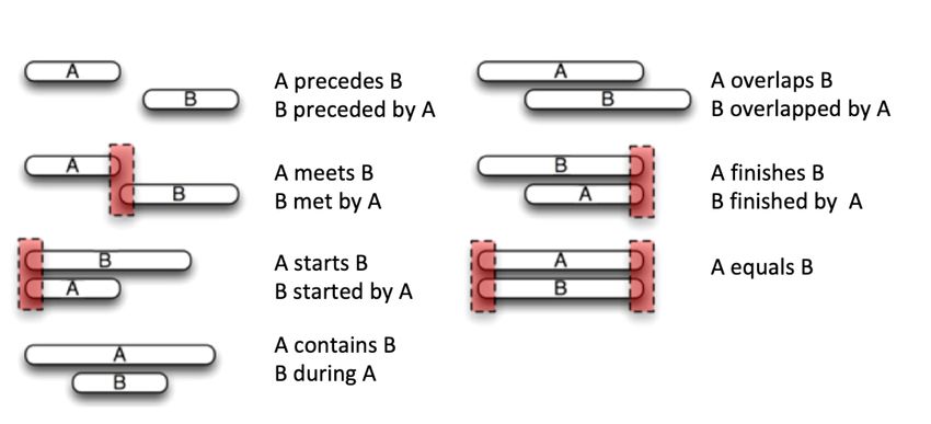
24th European Conference on Artificial Intelligence - ECAI 2020
Santiago de Compostela, Spain
(a) (b)
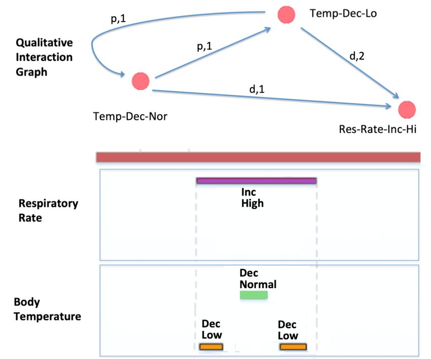
Figure 1: (a) Allen’s base seven temporal relations and their inverses. (b) The conceptual neighbourhood created by enforcing temporal con-
tinuity over Allen’s 14 relations. The conceptual neighbourhood graph shows the permitted transitions from one relation to another while
preserving temporal continuity. In the figure: p: precedes; m: meets; o: overlaps; s: starts,;d: during; f: finishes; pi: proceded by; si: started by;
mi: met by; oi: overlapped by; di: contains; fi: finished by; eq: equals.
The importance of the framework lies in its ability to extract intu- the intersection, union, and composition of a pair of temporal rela-
itive and multi-variable patterns of deviation from normal behaviour, tions [?]. Allen’s algebra enforces the notion of temporal continu-
capturing rare events in highly-dimensional, multivariate and non- ity via the relations’ conceptual neighbourhood [?]. In a conceptual
uniformly sampled data. The framework retains all the useful infor- neighbourhood, two relations between pairs of events are concep-
mation required for outcome prediction without jeopardising perfor- tual neighbours if they can be directly transformed into one another
mance. Moreover, and as opposed to the state of the art approaches, by continuous deformation (i.e., shortening or lengthening) of the
the framework can explain the outcomes predicted through the use of events. Allen’s conceptual neighbourhood structure is thus obtained
the aforementioned qualitative patterns. and is shown in Figure ?? (b). In the figure, the intervals are replaced
This paper is structured as follows. After discussing related work by circles containing the symbolic abbreviations of the names of the
in Section ??, we delve into the knowledge representation aspect corresponding relations as given in Figure ?? (a). Solid lines depict
of our work in Sections ?? and ??. We then formulate a pattern- neighbourhood relations. The conceptual neighbourhood distance
discovery model based on the Expectation-maximisation (EM) algo- between two qualitative relations quantifies the notion of temporal
rithm in Section ??. In Section ??, we evaluate the performance of continuity. It is defined as the shortest path between these relations
the pattern discovery model using sepsis as a case study and real ICU in the conceptual neighbourhood graph, giving every arc a distance
data. We perform two sets of experiments: while the first experiment being equal to one. Given two relations ri and rj , d(ri , rj ) is the con-
focuses on the discovery of significant interactions in a given pop- ceptual neighbourhood distance between the two relations and has a
ulation, the second is a classification experiment which verifies the minimum value of zero (when the two relations are the same).
ability of discovered interactions to discriminate patients who will In addition to using Allen’s algebra, most of the existing data
develop sepsis from those who will not, eight hours before onset. Fi- mining models use Shahar’s knowledge-based temporal abstraction
nally, we discuss the status of work and ongoing efforts in Section framework [?], which captures, among other properties, the qualita-
??. tive states (e.g. high, low, normal) and qualitative gradient changes
(e.g. increasing, decreasing, constant) during temporal intervals.
2 Related Work However, existing models that use qualitative temporal abstrac-
tions to mine time-series data, exemplified by [?, ?], have two vi-
The literature contains several data mining models that represent tal shortcomings. First, they individually mine qualitative state (e.g.
time-stamped multivariate raw data as a set of time intervals, often at high) and gradient (e.g. increasing) changes, without capturing the
a higher level of abstraction, and subsequently use discovered tem- richer semantics resulting from the simultaneous representation of
poral patterns for classification tasks [?, ?, ?, ?, ?, ?]. state and gradient changes as temporal patterns, and examining the
Most of these interval discovery models use Allen’s seminal work temporal interactions generated. This is especially vital for the med-
[?], which devises binary relations to capture the order and interac- ical domain (and the ICU in specific) where events are described by
tions between temporal intervals. Allen’s interval algebra contains multiple simultaneous qualitative descriptors. Second, they generally
a total of thirteen mutually-exhaustive and pairwise-disjoint qualita- focus on mining frequent temporal patterns, with the assumption that
tive relations, by which the temporal relationship between any two they are the highest contributors to a given outcome; an assumption
events can be unambiguously described. These relations are given in that does not hold in the medical domain as we illustrated in Sec-
Figure ?? (a). The set consists of six basic relations: precedes, meets, tion ??. Nevertheless, we build on the knowledge generated by these
starts, contains, overlaps, finishes, and their inverses: preceded by, approaches, using the knowledge-based temporal abstraction model
met by, started by, during, overlapped by and finished by. In the case of [?] as a foundation for defining the qualitative concepts used in
of the equal relation, the basic and inverse relations are identical. our work. In addition, we borrow the evaluation approach presented
The notion of an algebra over these relations arises from considering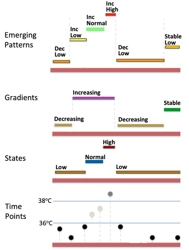
24th European Conference on Artificial Intelligence - ECAI 2020
                                                         Santiago de Compostela, Spain

in [?] to show that using our discovered interactions can be used as
features in classification problems to achieve high performance. Fi-
nally, we borrow the variable abstraction knowledge base of [?] in
the processing of our data in Section ??.
   The literature also contains models which aim at the discovery of
causal relations underlying a given large data [?, ?, ?, ?, ?]. How-
ever, many of the causality work requires the specification of prior
probabilities of events, which is not possible for many domains - for
example, in the ICU. To overcome the inference difficulties, causal
inference models using the expected values of domain variables to
detect rare events have been formulated [?], but are yet to take into
account the specific knowledge representation requirements of inten-
sive care. However, we acknowledge the importance and impact of
[?], and adapting its inference model to accommodate our knowledge
representation framework is part of our ongoing work.

3     Qualitative Interaction Graphs
The basic idea of the approach is to generate a set of patterns of
qualitative change embedded within time-series data and represent
their potential interactions via a graphical representation termed a
Qualitative Interaction Graph (QIG).

3.1     Knowledge-based Temporal Abstraction
       (KBTA)
Given time-stamped raw data grouped by objects of interest (e.g. a
patient’s ICU stay) and comrpising a set of temporal domain vari-
ables V (e.g. all vital signs recorded in an ICU over a period of time),
a set of abstract interval-based concepts are obtained for the ob-
ject of interest by exploiting domain-specific knowledge. We use the
knowledge-based temporal abstraction (KBTA) model introduced by             Figure 2: A series of raw time-point data for a patient’s body temper-
Shahar [?]. The model uses cut-off values suggested in a context-           ature is presented at the bottom. The data in this case are abstracted
sensitive fashion by a domain expert to determine maximal intervals         according to their values into four interval-based states (layer 2 from
whereby qualitative state changes (low, normal, high, e.g. high heart       the bottom), and into four gradient abstractions (layer 3 from the bot-
rate) as well as qualitative gradient changes (increasing, decreasing,      tom). The resulting temporal patterns combining state and gradient
stable, e.g. decreasing respiratory rate) hold. The bottom three layers     abstractions are shown in the top layer of the figure. There are exactly
of Figure ?? show an example of KBTA for body temperature. The              six temporal patterns resulting from the joint abstractions of state and
numerical values are given in the lowest level of the figure, while         gradient changes.
the second and third levels show the state and gradient abstractions
respectively.                                                               given patient), we distinguish a qualitative pattern from a qualita-
                                                                            tive pattern template. Patterns are aggregated into pattern templates
                                                                            such that two patterns map to the same template if they have the
3.2     Pattern Creation
                                                                            same qualitative state and gradient descriptions. Therefore, for a sin-
Maximal intervals of qualitative state-gradient pairs are aggregated        gle variable, the corresponding set of pattern templates comprises
into a sequence of temporally-contiguous patterns, such that within         unique qualitative state-gradient descriptors. For now, the start and
each pattern, the same state and gradient relations hold during the         end time of a template is the enumeration of the start and end times
pattern’s interval, but not immediately before or after the interval.       of the patterns making up the template. In Figure ??, two patterns of
The state-gradient temporal patterns abstracting body temperature           Decreasing-Low map to the same pattern template, resulting exactly
are shown in the top layer of Figure ??. In the figure, the interval dur-   five pattern templates in the figure: Decreasing-Low, Increasing-
ing which the gradient abstraction Increasing holds results in three        Low, Increasing-Normal, Increasing-High, and Stable-Low.
qualitative state-gradient patterns, by combining the gradient abstrac-
tion with the state abstractions that hold during the same interval.
The resulting patterns are: Increasing-Low, Increasing-Normal and
                                                                            3.4    Generating Qualitative Interaction Graphs
Increasing-High shown in the top layer of the figure.                       Given a set of temporal domain variables V , such that the state-
                                                                            gradient abstractions of each variable Vz ∈ V correspond to a set
                                                                            pattern templates Pz , qualitative temporal relations between pattern
3.3    Pattern Template Creation
                                                                            templates of different variables gives rise to a qualitative interaction
For each single variable (e.g. body temperature) Vz ∈ V where               graph G = (P, R). Figure ?? shows the creation of a QIG (top of the
V is the set of temporal domain variables for an object of interest         figure) from pattern templates of body temperature and respiration
(e.g. all vital signs recorded in an ICU over a period of time for a        rate (bottom of the figure). A QIG G has the following properties:
24th European Conference on Artificial Intelligence - ECAI 2020
Santiago de Compostela, Spain
1. G is a connected node and edge-labelled multi-graph in which the a given collection of variables, by first enumerating all pattern tem-
nodes P in which each node correspond to all pattern templates of plates and then generating subgraphs of increasing number of nodes
all temporal variables of interest extracted from the data timeline to some fix bound (for a total of n subgraphs in the lexicon). Using
of a given object, and the edges R correspond to the qualitative the subgraph lexicon, the structure of a qualitative interaction graph
temporal relations holding between any two pattern templates. of a single object i (e.g. patient) can be represented via a multi-hot
2. Interactions among variables are captured by the temporal re- vector of length n:
lationships between their corresponding pattern templates. The
edges reflect the semantics of the corresponding interaction via: θ(Gi ) = [li(k) ⊆ Gi ; ∀k ∈ 1...n]
(a) Edge labels, which describe the qualitative temporal relation
The multi-hot encoding of a given graph captures the structural
connecting the interacting pattern templates.
properties of the graph as described by the graph lexicon. When eval-
(b) Edge weights, which capture the frequency of a given interac- uating the similarity of the two graphs (e.g. to evaluate the similarity
tion between two templates. of the treatment journeys of two patients), we not only account for the
3. G a multi-graph, with multiple edges between two pattern tem- extent to which they share subgraphs (captured by their correspond-
plates denote different temporal interactions between the two tem- ing multi-hot vectors), but also take into account the semantics of
plates. the interactions, captured by the weights and labels of the subgraph
4. G is a directed graph, preserving the semantics of Allen’s interval edges. For any two edges, we define their similarity as:
relations. We use Allen’s seven base relations described in Figure
??. This means that we do not use inverse relations (as they are 1
implicitly defined by edge reversal), and limit the before relation sim(Ei , Ej ) = Ej Ej × (1)
d(ri , rj ) + |wi − wj | + 1
by a maximal allowed gap, as previously done in [?, ?].
Where Ej Ej denotes the correspondence between the nodes
Therefore, the structure of a QIG captures the simultaneous connecting each edge, and results in 1 when the nodes connecting the
change in state and gradient abstractions of the domain variables for two edges are the same, and zero otherwise. d(ri , rj ) is the concep-
a given object (e.g. patient). tual neighbourhood distance between the temporal relations ri and
rj (labeling edges Ei and Ej respectively) described in Section ??.
This enables the similarity function sim to take into account vary-
ing degrees of similarity, with the maximum value being 1 (when
the two edges are labeled with the same temporal relation, making
d(ri , rj ) = 0, and have equal weights, making |wi − wj | = 0).
We can therefore define the similarity vector of two graphs Gi and
Gj representing the normalised similarity of the subgraphs embed-
ded in the two graphs’ multi-hot vectors:
P
Ev ∈Gi sim(Ev , Ew )
Ew ∈Gj
Θ(Gi , Gj ) = [
|R(Gi )|
, if θ(Gi )k = 1 ∧ θ(Gj )k = 1; ∀k ∈ 1...n] (2)
Normalising the similarity of two subgraphs in the above equa-
tion, by dividing it by their mutual number of edges R(Gi ), guar-
antees that the similarity value will be in the range [0, 1] and is not
influenced by the size of the subgraphs at position k.
Finally, the similarity between two graphs S(Gi , Gj ) → [0, 1] is
the normalised sum of the two graphs’ similarity vector.
Figure 3: A Qualitative Interaction Graph connecting the pattern tem-
plates of respiratory rate and body temperature. There are two pat- n
X
terns which map to the same pattern template: Temp-Dec-Low; both Θ(Gi , Gj )
occur during the Res-Rate-Inc-Hi template, rendering the connecting k=1
S(Gi , Gj ) = (3)
edge weight 2. n
5 A Framework for Uncovering Rare Interactions
4 Describing and Comparing Qualitative
Interaction Graphs The aim of this work is to establish the grounds for finding interac-
tions that are embedded within a temporal dataset, and have the high-
We follow an approach where a qualitative interaction graph is de- est contribution to generating a given outcome. In order to distinguish
scribed by a collection of subgraphs, where each subgraph captures such significant interactions from all other interactions which may
several possible temporal interactions between subsets of qualitative indicate normal functioning or spurious events, the following model
templates as described in Section ??. We begin by populating a sub- is assumed to underlie the generation of significant interactions for
graph lexicon li of n elements, to contain all possible subgraphs for the domain of interest.24th European Conference on Artificial Intelligence - ECAI 2020
Santiago de Compostela, Spain
5.1 Prior Distribution Over Pattern Templates number of records in the raw dataset. Another note is that the func-
tions N and W used to partially compute Q are linear with respect
We describe the underlying prior probability distribution P (G) over to a given interpretation I.
sets of potential interaction subgraphs G = {G1 , ....Gm } as an ex- For the M-step, we estimate the values of the parameters λ1 − λ3
ponential distribution: and functions fλ1 − fλ3 that maximize Q(λ):
P (G) = exp(−λ1 W(G) + λ2 N (G) + λ3 F(G)) (4) λmax = arg max Q(λ, λ∗ )
The description of the distribution reflects the characteristics that Upon convergence of the EM procedure, we sample the distri-
we would like our potential target interactions to possess. First, the bution of interpretations to obtain the significant interactions of the
distribution favours interactions with small weights, as larger weights model, giving preference to interpretations interpretations with lower
signal interactions that are more frequent with respect to a given ob- mean edge weight.
ject (e.g. patient), and those are less likely to have caused the out- Because iterating over the set of all possible interpretations via the
come, as described in the introduction. Hence the exponentially de- EM algorithm is also infeasible, we include a pre-processing step to
creasing function of W(G), which returns in the average weight of a obtain clusters of interpretations that are likely to be optimal, using
given subgraph. the graph lexicon to cluster the interaction graphs embedding the in-
Second, the distribution favours larger interaction subgraphs, teractions within the data using self-tuning spectral clustering [?].
which is reflected by the exponentially increasing function of N (G).
This may seem counter intuitive, going against the observations con-
6 Experimental Evaluation
cerning the medical domain, where the number of variables leading
to an outcome is orders of magnitude less than the number of vari- Our experiments are based on the discovery and evaluation of inter-
ables measured. However, we will make the reasoning behind this actions that can best explain a given outcome. To achieve this, we
clear after examining the third component of the distribution. organise our evaluation into two steps:
Finally, the distribution favours subgraphs with maximum
favouritism with respect to the population, which is calculated by 1. Pattern Discovery: by using the model presented here to discover
aggregating its similarity to other graphs in the population: significant patterns describing a population of subjects with a
Y given outcome, comparing the generated patterns with those gen-
F(G) = log( S(G, Gz )) (5) erated by existing temporal pattern discovery models.
Gz ∈G 2. Outcome Discovery: by using the discovered patterns as predic-
tors of a given outcome in a classification experiment, and com-
Hence the final component describing the distribution is an expo- paring the performance against those of a number of classification
nentially increasing function of F(G). machine learning algorithms whose performance is established for
Although the second component N favours larger subgraphs, its the given domain problem.
effect is smoothed by the third component F, because as subgraphs
become larger, the likelihood of finding similar subgraphs in the pop-
ulation decreases. In fact, the two competing functions N and F 6.1 The Medical Problem
force the distribution to generate smaller subgraphs to achieve a high
favouritism score. Sepsis, defined by a life-threatening response to infection and poten-
The parameters of the independent components of the distribution tially leading to multiple organ failure, is a devastating condition and
are used to find the optimal significant interactions of a (latent) out- one of the most significant causes of worldwide morbidity and mor-
come for a given dataset, as described in ?? below. tality [?]. Sepsis is implicated in 6 million deaths annually, with costs
totaling $24 billion in the USA alone [?].
Early identification of sepsis is a known crucial factor in improv-
5.2 Parameter Estimation ing its outcomes [?]. Yet, existing sepsis prediction models using ma-
chine learning have shown mixed results reflecting the difficulty in
Since enumerating all possible interactions and evaluating their sig- pinpointing the factors leading to sepsis onest [?], and heterogeneity
nificance is infeasible, the EM algorithm [?] is applied to estimate the in populations [?] and methodologies [?].
parameters of the distribution and use those to find significant inter- Recently [?] proposed a temporal data mining approach using gra-
pretations of the model. An interpretation I is a subgraph containing dient and state abstractions of temporal intervals to find the most fre-
a subset of the interactions in a population of qualitative interaction quent patterns in a population of septic patients. Comparing those to
graphs G. There are three parameters in the model: λ1 − λ3 . Along temporal patterns in non-septic patients found significant statistical
with the three generative functions fλ1 − fλ3 , they define the dis- differences. The work does not evaluate the ability of the discovered
tribution generating significant interactions as per Equation ??. The patterns to perform sepsis prediction; a task which we perform as
expected value of the log likelihood function Q(λ, λ∗ ) becomes: part of our evaluation.
m X
3
6.2 The Dataset
X
Q(λ, λ∗ ) = Eλ∗i (log fλi (I)|Gk )
k=1 i=1
We used the Medical Information Mart for Intensive Care III
m is the total number of generated graphs, which correspond to the (MIMIC-III) [?], a large and freely-accessible de-identified inten-
number of objects in the dataset (see Section ??). Since each object sive care database from Boston, Massachusetts, USA. MIMIC-III
is described by many records (with each record corresponding to a contains demographics, vital sign measurements, laboratory test re-
time-stamped value for a given variable), m
M, where M is the sults, procedures, medications, caregiver notes and imaging reports24th European Conference on Artificial Intelligence - ECAI 2020
Santiago de Compostela, Spain
recorded over time, in addition to mortality data (both in and out of to [?]). We re-queried the dataset to only include vitals which have
the hospital) for over 46,520 critical care patients. been recorded over 8 hours before the confirmation of sepsis was
We processed the data contained within MIMIC-III to exclude: recorded in the patient’s records. We used the 2,360 records allo-
1. non-adults, less than 15 years of age at the time of admission, cated to pattern discovery, which were all septic patients. After fil-
2. invalid admissions, which frequently correspond to clerical errors tration, 1,679 records satisfied the temporal constraint enforced on
and are characterised by the absence of heart rate, incomplete ad- the records. Summary of the discovered interactions is given in Ta-
ministrative recordings or admission and discharge and no charted ble ??. In the table, the first column describes the sampling rate: the
observations, and 3. stays shorter than 4 hours, as those tend to have percentage of significant interactions sampled from the distribution
high rates of incomplete data and are therefore of little value for our of interpretations after the convergence of the EM procedure of Sec-
purpose. We then queried the MIMIC-III database for patients sat- tion ??. The second column shows the number of patterns discovered
isfying the conditions the third international definition of sepsis [?], using the corresponding sampling rate in the first column. The third
under the guidance of two domain experts, and using surrogates of column describes the percentage of septic patients with the sampled
an organ dysfunction component of acute increase in SOFA score patterns being subsets of their qualitative interaction graphs, while
beyond 2 points and persistent hypotension (mean blood pressure < the fourth column describes the same percentage non-septic patients.
65) requiring vasopressors to maintain mean arterial pressure. The table clearly shows that the top 5% of the discovered inter-
The resulting set comprises 4,720 ICU records for 4,403 patients actions are almost only exclusively found in the septic population.
(a single patient may have multiple ICU visits). We divided the Moreover, comparing these results with the temporal patterns dis-
records into two sets of 2,360 ICU records each. The first set will covered via frequent pattern mining in [?] shows the clear contrast
be used for pattern discovery, while the second will be used for eval- in the two approaches and highlights the advantages of searching for
uation. In addition, we extracted an equivalent 2,360 records from rare interactions. [?] found a total of 6,168 patterns with exclusive
the records that did not satisfy our inclusion criteria to serve as nega- prevalence in the septic population and 14,384 patterns found to be
tive examples for the classification experiments of our evaluation. We present in both septic and non-septic patients.
extracted the variables shown in Table ?? and used the state and gra-
dient abstraction cutoffs shown in the table to abstract the raw data Table 2: The distribution of significant patterns across septic and non-
into more meaningful concepts. The knowledge base given in the ta- septic patients
ble is an exact replica of that used in previous work using temporal
knowledge-based temporal abstraction to prediction sepsis [?]. Sampling Number of Prevalence in Prevalence in
Rate Patterns Septic Patients Non-septic Patients
5% 39 99% < 0.05%
Table 1: The knowledge base detailing the variables and state and
10% 75 94.8% 0.08%
gradient cutoff values for temporal abstraction of ICU vitals and lab- 40 % 302 0.82% 0.2%
oratory tests 80% 610 0.79% 0.26%
Clinical ’Normal’ State Gradient
Concept Abstraction Abstraction We note that the visible improvement in the number and discrim-
Albumin 3.4-5.4 g/dL ∆ > 0.5 inatory power of the discovered interactions is achieved despite the
Bilirubin 0.2 - 1.2 mg/dL ∆ > 0.5
chloride 96 106 mEq/L ∆ >5 fact that our EM procedure is unsupervised, and was only given a
Fibrinogen 200 400 mg/dL ∆ > 50 population of septic patients (no negative examples or labeling per-
Creatinine 0.6-1.3 mg/dL ∆ > 0.2 formed). This is in contrast to [?], which performed the pattern dis-
Glucose 70 100 mg/dL ∆ > 10 covery process using clearly labeled sepsis and non-sepsis records.
Hemoglobin 11 18 g/dL ∆ >2
Given the stark difference in discriminatory power of discovered
Lactate 0.5 - 2.2 mmol/L ∆ >1
PCO2 38 42 mm Hg ∆ >2 interactions, we argue that the QIG model not only enables the dis-
Urea 10 20 mg/dL ∆ >5 covery of more useful interactions, but the semantics of the model
Sodium 135 145 mEq/L ∆ >5 captured by the joint representation of qualitative state and gradi-
TCO2 22 28 mmol/l ∆ >2 ent change highly contribute to the derivation of a smaller and more
WBC 4.5 10 × 109 /L ∆ >1
Body Temperature 36 38 ◦ C ∆ >0.5 meaningful set of significant interactions.
Glasgow Coma Scale 8-12 ∆ >2
Diastolic Blood Pressure 70 90 mmHg ∆ >10 Table 3: Prevalence of interaction subsets in the QIG most significant
Systolic Blood Pressure 110 140 mmHg ∆ >10 patterns
Mean Blood Pressure 65 - 80 ∆ >5
Heart Rate 60 80 bpm ∆ >10
Spontaneous Respiratory Rate 7 14 breath/pm ∆ >3 Node 1 Node 2 Temporal Rel Prevalence
Platelets 150 400 × 109 /L ∆ > 50 SysBP-Low-Dec Temp-Hi-Incr Finishes 77%
PO2 (PaO2 in Andrea) 75 100 tor ∆ >10 WBC-Norm-Inc Temp-Hi-Incr Overlaps 61%
PCO2 (PaCO2 in Andrea) 38 42 mm Hg ∆ >2 Heartrate-Hi-Stab Temp-Hi-Stab Overlaps 49%
Lactate-Hi-Stab Heartrate-Hi-Stab During 35%
We further examined the top 5% (39) patterns discovered by our
6.3 Experiments and Results QIG model for the clinical significance of the most prevalent subsets
of interactions. These are given in Table ??.
6.3.1 Discovering Significant Sepsis Patterns
Close examination of the most prevalent interaction subsets (with
This experiment aims to discover significant patterns of interactions the help of two domain experts) show that the variables and the or-
within the septic population 8 hours prior to sepsis onset (similarly der of their changes in the interactions is semantically meaningful24th European Conference on Artificial Intelligence - ECAI 2020
Santiago de Compostela, Spain
Table 4: Comparison of performance metrics of the QIG model in predicting sepsis 8 hours prior to ICU admission, with the performance of
state of the art sepsis prediction models obtained from the literature. AUROC: Area Under the Receiver-operator Curve. PLR: Positive Like-
sensitivity 1 − sensitivity
lihood Ratio ( ), NLR: Negative Likelihood Ratio ( ). Note: * indicates values calculated using the reported
1 − specif icity specif icity
sensitivity and specificity.
Model Sensitivity Specificity AUROCC PLR NLR
(95% CI) 95% CI (95% CI) (95% CI)
QIG 0.98 (0.96-0.99) 0.95 (0.91 - 0.99) 0.97 19.6 0.02
Kam 0.94 (0.93-0.95) 0.91 (0.88-0.94) 0.929 10.45∗ 0.07∗
Mao 0.98 (0.96- 0.99) 0.8 (0.78-0.82) 0.915 4.90∗ 0.03∗
Desautels 0.80 (0.79-0.81) 0.79 (0.780.81) 0.791 3.8∗ 0.25∗
Nemati 0.85 (0.84 - 0.86) 0.84 (0.82 - 0.86) 0.85 5.3∗ 0.18∗
Calvert 0.9 (0.890.91) 0.81 (0.800.82) 0.86 4.7∗ 0.12∗
from a clinical perspective. For instance, the first pattern describes noting that the improved performance of the QIG model is especially
periods where a patient has a low and consistently decreasing sys- pronounced in the specificity of predictions, in which more explain-
tolic blood pressure, such that these periods are temporally equiv- able models (Mao) underperforms by not distinguishing septic pa-
alent (in a qualitative sense) to the finishing intervals of increasing tients from those with inflammations and comorbidities; a general
high temperature. Clinically, having a high temperature is one of the bottleneck in ML sepsis prediction [?]. It is also worth noting that
first alarming signs in an ICU patient and is a valid reason to look only [?] claims to be a fully interpretable model (by virtue of feature
for signs of infections. As the possibility of an infection increases in importance).
a given patient, her other vitals start showing signs of deterioration,
and a low and decreasing Systolic blood pressure is one of the first 7 Conclusions, Limitations and Future Work
to show significant values changes. Similarly, increasing (yet still in
the normal range) white blood cell count indicate that the body is In this work, we have proposed a framework for the discovery of
preparing to fight an infection. However, if fever develops during this rare patterns of interactions from highly-dimensional, multivariate
period of incremental increase in WBC count, this may indicate that and non-uniformly sampled time series data. The model uses quali-
the body is in alarm mode and an infection maybe imminent. tative abstraction to capture meaningful semantics embedded within
the raw data and formulates a probabilistic model governing rare in-
teractions. We used an expectation-maximisation procedure to un-
6.3.2 Using Significant Patterns as Predictors of Sepsis cover temporal interactions with the highest contributions to a given
outcome. The paper presents experiments using the framework on
Using the set of 2,360 ICU records of septic patients not used in real ICU data to discover rare temporal interactions contributing to
pattern discovery as positive examples, and the 2,360 ICU records the onset of sepsis. The results show that using the patterns identi-
of non-septic patients as negative examples, and further filtering the fied by our model as features in classification experiments yields a
data to exclude variables recorded less than 8 hours of confirmed superior discriminatory power to when using the raw data, as well as
sepsis diagnosis, we performed a classification task with sepsis di- superior performance to state of the art machine learning algorithms
agnosis as outcome and using the top 10% interaction patterns as that have been specifically optimised for sepsis prediction.
features for the learning task (for a total of 39 features). Using the Our present research focuses on a number of areas of improve-
XGBoost classification algorithm, the classifier’s parameters were ment. To begin with, QIGs learned from the data can be further op-
optimised through a bootstrapped grid search over is hyperparam- timised using the topological constraints of Allen’s relations to re-
eter space. After filtering the records by time, our dataset contained a move redundant labels by inferring them from the graph [?]. More-
substantial class imbalance (only 36% positive examples). We there- over, using a multi-resolutional representation of time to create QIGs
fore employed cost-sensitive learning by placing a heavier penalty on can accommodate imprecise, gradual and intuitive relations between
misclassifying the minority class (septic patients). The classifier was points and intervals [?]. We are also designing a causal rare event
training over 1,000 iterations of a 10-fold cross-validation, incorpo- discovery framework exploiting the rich semantics captured by our
rating class weights into each. representation. Finally, we are working on the algorithmic aspects
In addition to the performance metrics of the QIG-based classifier of pattern discovery to devise efficient and scalable algorithms for
reported in Table ??, we collected the reported performance met- the fast detection of rare temporal interactions, overcoming the slow
rics of five models representative of current sepsis predictors: [?] EM algorithm implementation, which is far from the ultimate goal of
(referred to as Kam), [?] (referred to as Mao), [?] (referred to as De- real-time monitoring.
sautels), [?] (referred to as Nemati), and [?] (referred to as Calvert).
Indeed, the results underline the current bottleneck of ML-based sep-
sis prediction: the highest performance of the models available in the 8 Acknoweldgements
literature was reported by Mao and Kam. Mao relies on feature se- We sincerely thank Andrea Agarossi and Ahmed Hamoud for their
lection to achieve performance, but only reports high sensitivity at valuable insight and domain expertise. This research was supported
the fixed specificity value of 0.8. In contrast, Kam is a neural net- by the following funding bodies:
work model which does not perform explicit feature selection. While
it reports high sensitivity and specificity, the black-box nature of the 1. Health Data Research UK, which is funded by the UK Medical
Kam model hinders its clinical utility in practical settings. It is worth Research Council, Engineering and Physical Sciences Research24th European Conference on Artificial Intelligence - ECAI 2020
Santiago de Compostela, Spain
Council, Economic and Social Research Council, Department of
Health and Social Care (England), Chief Scientist Office of the
Scottish Government Health and Social Care Directorates, Health
and Social Care Research and Development Division (Welsh Gov-
ernment), Public Health Agency (Northern Ireland), British Heart
Foundation and Wellcome Trust.
2. The National Institute for Health Research University College
London Hospitals Biomedical Research Centre.
3. National Institute for Health Research (NIHR) Biomedical Re-
search Centre at South London and Maudsley NHS Foundation
Trust and Kings College London.
4. The UK Medical Research Council (MRC), grant numbers
MR/S004149/1 and MC PC 18029.You can also read