MODULATION SPECTRAL SIGNAL REPRESENTATION AND I-VECTORS FOR ANOMALOUS SOUND DETECTION - dcase
←
→
Page content transcription
If your browser does not render page correctly, please read the page content below
Detection and Classification of Acoustic Scenes and Events 2020                                                                             Challenge

                            MODULATION SPECTRAL SIGNAL REPRESENTATION
                           AND I-VECTORS FOR ANOMALOUS SOUND DETECTION
                                                                  Technical Report

                               Parth Tiwari1 3 , Yash Jain2 , Anderson Avila3 , João Monteiro3 ,
                                    Shruti Kshirsagar3 , Amr Gaballah3 , Tiago H. Falk3
                      1
                Department of Industrial and Systems Engineering, IIT Kharagpur, India
                           2
                             Department of Mathematics, IIT Kharagpur, India
       3
         MuSAE Lab, Institut National de la Recherche Scientifique - Centre EMT, Montreal, Canada

                             ABSTRACT                                       system. The features are extracted from the so-called modulation
                                                                            spectrum (MS) signal representation, which quantifies the rate of
This report summarizes our submission for Task-2 of the DCASE               change of the signal spectral components over time. These features
2020 Challenge. We propose two different anomalous sound de-                have previously been useful for stress detection in speech [2], for
tection systems, one based on features extracted from a modula-             speech enhancement [3], and room acoustic characterization [4], to
tion spectral signal representation and the other based on i-vectors        name a few applications.
extracted from mel-band features. The first system uses a nearest              In our second system, in turn, we use i-vectors and Gaussian
neighbour graph to construct clusters which capture local varia-            Mixture Models (GMM) for anomaly detection. i-vectors have been
tions in the training data. Anomalies are then identified based on          widely used for speech applications, including speech, speaker, lan-
their distance from the cluster centroids. The second system uses           guage, and accent recognition. We extract i-vectors from MFCC
i-vectors extracted from mel-band spectra for training a Gaussian           features and use them to train GMMs for anomaly detection. The
Mixture Model. Anomalies are then identified using their negative           negative log likelihood for a sample is used as its anomaly scores.
log likelihood. Both these methods show significant improvement             Lastly, an ensemble of these two systems is also experimented with.
over the DCASE Challenge baseline AUC scores, with an average
improvement of 6% across all machines. An ensemble of the two
systems is shown to further improve the average performance by                                 2. SYSTEM DESCRIPTION
11% over the baseline.
                                                                            2.1. System 1 - Graph Clustering using Modulation Spectro-
  Index Terms— i-Vectors, Amplitude-Modulation Spectrums,                   grams
Graph, Clustering, Gaussian Mixture Models
                                                                               2.1.1. Pre-processing and Feature Extraction
                          1. INTRODUCTION                                   Modulation spectrum corresponds to an auditory spectro- temporal
                                                                            representation that captures long-term dynamics of an audio signal.
Monitoring industrial machinery can prevent the production of               The pipeline proposed in [5] is used to extract modulation spectro-
faulty products and decrease the chances of machine breakdown.              grams.
Anomalous sounds can indicate symptoms of unwanted activity,                    Prior to feature extraction, noise reduction is performed on the
hence, Anomalous Sound Detection (ASD) systems can potentially              signal through a spectral gating method (using noisereduce1 in
be used for real time monitoring of machines. Unsupervised ASD              Python), described as follows: 100 normal training sound clips for
systems rely on only “normal” sounds for identifying anomalies.             a machine-id are averaged and used as a noise clip for that machine-
Developing ASD systems in an unsupervised manner is essential,              id. An FFT is calculated over this noise clip and statistics including
as: (i) the nature of anomalies may not be known beforehand, and            the mean power, are tabulated for each frequency band. A threshold
(ii) deliberately destroying expensive devices is impractical from a        for each frequency band is calculated based upon the statistics. An
development cost perspective. In addition, the frequency at which           FFT is calculated over the signal. A mask is determined by com-
anomalies occur is low and the variability in the type of anomaly is        paring the signal FFT to the threshold. The mask is smoothed with
high, therefore, developing balanced datasets for supervised learn-         a filter over frequency and time. The mask is appled to the FFT of
ing is difficult.                                                           the signal, and is inverted.
    In our proposed systems, we focus on using features which are               The speech activity level is normalized to -26 dBov (dB over-
able to capture anomalous behaviour. Simple machine learning al-            load), after noise removal thus eliminating unwanted energy varia-
gorithms when used on top of these features are able to beat the            tions caused by different loudness levels in the speech signal. Next,
baseline performance[1]. In our first system, we propose an outlier         the pre-processed speech signal x̂(n) is filtered by a 60-channel
detection method which is similar to a nearest neighbour search. In         gammatone filterbank, simulating cochlear processing [6]. The first
this method, clusters of normal sounds are formed using a nearest           filter of the filterbank is centered at 125 Hz and the last one at at just
neighbour graph to capture variations in the normal working sounds          below half of the sampling rate. Each filter bandwidth follows the
of a machine. Anomalies are then identified based on their distance
from these clusters. Modulation spectrum features are used for this            1 https://pypi.org/project/noisereduce/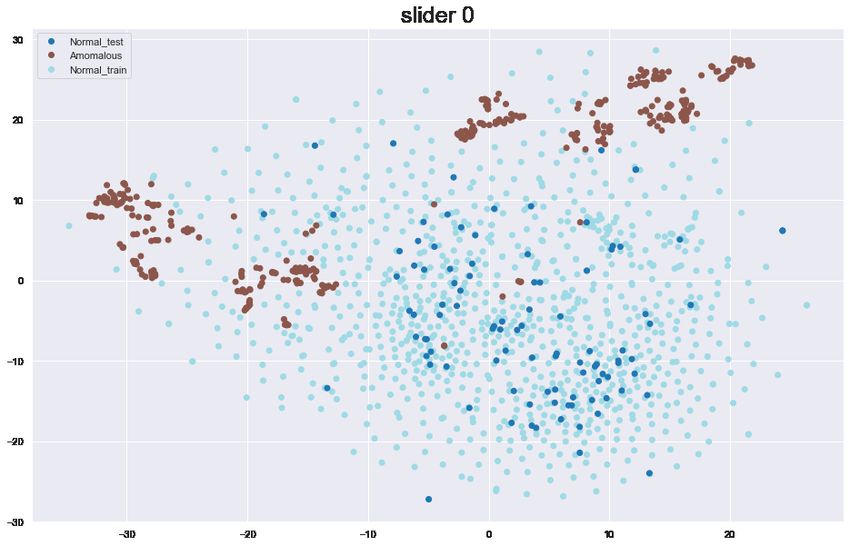
Detection and Classification of Acoustic Scenes and Events 2020                                                                      Challenge

                        Figure 1: Block diagram describing steps for computing the modulation spectral representation

                                                                          Figure 3: Modulation spectrograms for four normal training sam-
Figure 2: Frequency responses of the 8-channel modulation filter-
                                                                          ples from Pump machine-id 2
bank

equivalent rectangular bandwidth (ERB), which is an approxima-            all our experminets. This results in a 60 × 8 modulation spectral
tion of the bandwidths of the filters in human hearing, as described      representation (i.e., modulation spectrogram) for each sound clip.
below:
                                     fi                                     2.1.2. Anomaly Detection
                        ERB j =           + B min ,                 (1)
                                    Qear
                                                                          Figure 3 shows four modulation spectrograms for the normal train-
where f j represents the center frequency of the j-th filter. Qear rep-
                                                                          ing samples of Pump machine-id 2. It can be seen that a significant
resents the asymptotic filter quality at high frequencies and B min is
                                                                          amount of variability exists within the same machine-id. We capture
the minimum bandwidth for low frequencies. They are set, respec-
                                                                          this variability by a graph-based clustering approach using modula-
tively, to 9.265 and 24.7.
                                                                          tion spectra as features.
   The temporal envelope ej (n) is then computed from x̂j (n), the
output of the j-th acoustic filter, via the Hilbert transform:                 Consider a graph G = (V, E) where V is the set of nodes
                                                                          comprising of the normal training sound clips. E is the set of
                  ej (n) = x̂j (n)2 + H {x̂j (n)}2
                           p
                                                                    (2)   edges connecting the nodes. Two nodes v p , v q ∈ V share an edge
                                                                          epq ∈ E such that q = argmin({ D(v p , v r ) | r = 1, .., p −
where H {.} denotes the Hilbert Transform. Temporal envelopes             1, p + 1, ...|V | }). Here D(v p , v r ) is the L1 distance between
ej (n), j = 1, ..., 60 are then windowed with a 256-ms Hamming            v p , v r . The graph G, when constructed in this manner, consists of
window and shifts of 40 ms. The discrete Fourier transform F {.}          several disjoint subgraphs i.e. G = g 1 ∪ g 2 ∪ g 3 ...g n such that
of the temporal envelope ej (m; n) (m indexes the frame) is then          g l ∩ g m = φ ∀ l, m = 1, 2, ...n | l 6= m. Each of these sub-
computed in order to obtain the modulation spectrum E j (m, f m ),        graphs is treated as a separate cluster. A centroid µl and standard
i.e.,                                                                     deviation σ l are calculated corresponding to each cluster by taking
                                                                          the mean and standard deviation of all frequency bins. µl , σ l both
                    E j (m; f m ) = kF (ej (m; n))k                (3)    have dimensions 60 × 8. This graph G and the corresponding clus-
where m represents the m-th frame obtained after every Hamming            ter centroids, standard deviations are computed separately for each
window multiplication and f m designates modulation frequency.            machine-id.
The time variable n is dropped for convenience. Lastly, following              Anomaly score for a sound clip of a machine-id is calculated
recent physiological evidence of a modulation filterbank structure        using the standard-deviation normalized distance from each cluster
in the human auditory system [6]. an auditory-inspired modulation         centroid corresponding to that machine-id. For a given sample in
filterbank is further used to group modulation frequencies into eight     the test dataset v t ∈ / V , its anomaly score At is given by At =
bands. These are denoted as E (j,k) (m), k = 1, ..., 8, where j indexes   min({z t,l | ∀ l})
the gammatone filter and k the modulation filter. Figure 3 depicts
                                                                                                        60 X
                                                                                                           8
the frequency response for the 8-channel modulation filterbank used                                    X     |z t,j,k − µl,j,k |
                                                                                             z t,l =                             .          (4)
in our system. Note that the filter center frequencies are equally                                                   σ t,j,k
                                                                                                       j=1 k=1
spaced in the logarithmic scale from 4 to 128 Hz. The modulation
spectral representation frames obtained over time are averaged for          Here, z t,j,k is the energy value at the jth gammatone filterbank
Detection and Classification of Acoustic Scenes and Events 2020 Challenge
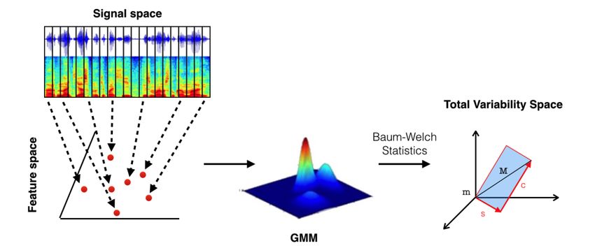
Figure 4: Diagram describing the steps for i-vector extraction
and kth modulation filterbank. The intuition behind this strategy for
finding anomaly scores is that normal samples will lie closer the one
of the cluster centroids in comparison to anomalous samples. This Figure 5: 2D t-SNE projections of i-Vectors corresponding to
method does not require any training and can be seen as a KNN machine-slider, machine-id 0
based ASD system where instead of computing distances from each
training sample, we only find the distances from the cluster centroid.
where cn is the nth mel-cepstral coefficient and Ym refers to the
2.2. System 2 - GMMs using MFCC i-Vectors log-energy of the mth filter. In this work, a set of 13 coefficients
together with log energy, delta and delta-delta coefficients form the
2.2.1. Feature Extraction feature vector from each frame.
The i-vector framework maps a list of feature vectors, O =
{ot }N F
t=1 , where ot ∈ R , and N is the frame index. Typically
2.2.2. Anomaly Detection
Mel-frequency cepstral coefficients (MFCC’s) extracted from an ut- The 100 dimensional i-vectors extracted from the normal training
terance, into a fixed-length vector, n ∈ RD . In order to achieve sounds are used to train a Gaussian Mixture Model using scikit-
that, a Gaussian mixture model (GMM), λ = ({wk }, {mk }, {σk }), learn [11]. Ten mixture components are used for all machines with
is used. The GMM, trained on multiple utterances, is referred to each component having its own general full covariance matrix. The
as the universal background model (UBM), and is used to collect ability of i-vectors to capture anomalous behaviour is depicted in
Baum-Welch statistics from each utterance [7]. Such statistics are Figure 5. Here, 2D t-SNE embeddings show that i-vectors corre-
computed for each mixture component k, resulting in the so-called sponding to anomalous sounds are well separated from the normal
supervector M ∈ RF K , where F represents the feature dimension sounds. i-vectors seem to be spread according to a Gaussian den-
and K is the number of Gaussian components. As in the Joint Fac- sity, which is the key motivation behind using GMMs for anomaly
tor Analysis (JFA) [8], the i-vector framework also considers that detection.
speaker and channel variability lies in a lower subspace of the GMM The negative log-likelihood of sample x is given by:
supervectors [9]. The main difference between the two approaches
is that the i-vector projects both speaker and channel variability into K
X
the same subspace, namely total variability space, represented as −logP (x|π, µ, σ) = −log π k N(x|µk , σ k ) , (7)
follows: k=1
where π k is the mixing coefficient for the kth component of the
M = m + T w, (5)
GMM and µk , σ k are the corresponding mean and co-variance ma-
where M is the dependent supervector (extracted from a specific trices. These values are used as the anomaly score.
utterance) and m is the independent supervector (extracted from
the UBM), T corresponds to a rectangular low-rank total variability 2.3. System 3 - Graph–i-vector Ensemble
matrix and w is a random vector with a normal distribution, the so-
called i-vector. In our experiments, a 100-dimensional i-vector was Lastly, an ensemble of the two proposed system shows performance
adopted extracted on top of MFCC features. improvement in several cases. Anomaly scores obtained from the
Mel frequency spectrum coefficients - Prior to their extraction, the two systems are first normalized using their minimum and maxi-
input signals (sampled at 16 kHz) are normalized to -26 dBOV. The mum values. The ensemble anomaly scores are then computed by
signals also undergo a pre-emphasis filter of coefficient 0.95, which taking the geometric mean of the normalized values.
is meant to balance low and high frequency magnitudes. A 30-ms
Hamming window with 50% overlap is applied before extracting
3. RESULTS
the MFCCs. The Hamming window is used to remove edge effects
[10]. The cepstral feature vector can then be extracted from each The results are shown in Table 1. When trained on develop-
frame according to: ment data[12, 13], the graph clustering system outperforms the
M
baseline[1] by an average of 6% and 32% AUC for machines slider
cn =
X
[Ym ]cos
πn
m− 1
, n = 1, 2, 3, ..., N, (6) and valve respectively. The i-vector GMM system outperforms
M 2
m=1
baseline and graph clustering system for some of the machine IDsDetection and Classification of Acoustic Scenes and Events 2020 Challenge
Table 1: AUC and pAUC scores for all machines in the development dataset. Modspec Graph, iVGmm, Ensemble correspond to Systems
1-3, respectively. The best scores for each case have been shown in bold.
Baseline Modspec iVGmm Ensemble Baseline Modspec iVGmm Ensemble
Machine Mid
AUC Graph AUC AUC AUC pAUC Graph pAUC pAUC pAUC
1 81.36% 78.24% 75.04% 81.64% 68.40% 64.69% 57.54% 66.75%
2 85.97% 89.06% 83.30% 91.72% 77.72% 76.14% 67.00% 79.78%
ToyCar 3 63.30% 67.16% 79.47% 78.21% 55.21% 52.58% 59.52% 56.37%
4 84.45% 89.40% 94.84% 96.44% 68.97% 63.54% 82.94% 84.80%
Avg 78.77% 80.96% 83.16% 87.00% 67.58% 64.24% 66.75% 71.92%
1 78.07% 62.56% 55.51% 64.62% 64.25% 51.59% 52.82% 52.24%
2 64.16% 54.03% 53.80% 56.65% 56.01% 49.99% 50.95% 50.23%
ToyConveyor
3 75.35% 59.10% 59.09% 64.06% 61.03% 50.31% 52.82% 52.25%
Avg 72.53% 58.57% 56.13% 61.78% 60.43% 50.63% 52.20% 51.58%
0 54.41% 63.37% 67.85% 67.12% 49.37% 49.73% 57.38% 52.92%
2 73.40% 79.32% 70.39% 80.48% 54.81% 57.16% 61.93% 59.21%
fan 4 61.61% 71.76% 73.52% 78.07% 53.26% 50.68% 57.53% 53.99%
6 73.92% 74.00% 81.15% 81.90% 52.35% 49.38% 56.31% 49.23%
Avg 65.83% 72.11% 73.23% 76.89% 52.45% 51.74% 58.29% 53.84%
0 67.15% 86.66% 74.99% 86.95% 56.74% 82.52% 67.10% 78.32%
2 61.53% 62.44% 74.91% 70.06% 58.10% 64.77% 60.08% 65.72%
pump 4 88.33% 84.16% 92.02% 90.73% 67.10% 59.95% 73.74% 68.00%
6 74.55% 81.64% 71.10% 82.65% 58.02% 66.20% 51.70% 66.56%
Avg 72.89% 78.72% 78.26% 82.60% 59.99% 68.36% 63.15% 69.65%
0 96.19% 99.91% 83.92% 98.72% 81.44% 99.53% 50.04% 93.44%
2 78.97% 84.36% 56.93% 77.93% 63.68% 73.86% 47.84% 52.89%
slider 4 94.30% 97.83% 87.84% 95.93% 71.98% 88.59% 62.71% 79.69%
6 69.59% 79.03% 59.04% 71.40% 49.02% 55.47% 49.91% 52.28%
Avg 84.76% 90.28% 71.93% 86.00% 66.53% 79.36% 52.63% 69.57%
0 68.76% 100.00% 79.33% 98.80% 51.70% 100.00% 52.94% 95.62%
2 68.18% 99.88% 85.35% 98.69% 51.83% 99.34% 56.27% 93.29%
valve 4 74.30% 98.26% 84.10% 95.88% 51.97% 91.32% 56.32% 80.26%
6 53.90% 89.22% 69.84% 85.01% 48.43% 72.59% 49.91% 59.65%
Avg 66.28% 96.84% 79.65% 94.59% 50.98% 90.81% 53.86% 82.21%
in pump and fan. The ensemble of graph clustering system and i- sification based on modulation spectral features and convolu-
vector GMM system outperforms the baseline by an average AUC tional neural networks,” in 2019 27th European Signal Pro-
score of 8%,11% and 10% for machines ToyCar, fan, and pump, re- cessing Conference (EUSIPCO). IEEE, 2019, pp. 1–5.
spectively. Interestingly, the performance for the ToyConveyor case [3] S. Karimian-Azari and T. H. Falk, “Modulation spectrum
was lower than that achieved by the benchmark system for all three based beamforming for speech enhancement,” in 2017 IEEE
proposed systems. This may be due to anomalies which occur for a Workshop on Applications of Signal Processing to Audio and
very small time interval and are not being captured by the proposed Acoustics (WASPAA). IEEE, 2017, pp. 91–95.
longer-term features. We provide our implementation here2 .
[4] T. H. Falk and W.-Y. Chan, “Temporal dynamics for blind
measurement of room acoustical parameters,” IEEE Transac-
4. REFERENCES tions on Instrumentation and Measurement, vol. 59, no. 4, pp.
978–989, 2010.
[1] Y. Koizumi, Y. Kawaguchi, K. Imoto, T. Nakamura,
[5] T. H. Falk and W. Chan, “Modulation spectral features for
Y. Nikaido, R. Tanabe, H. Purohit, K. Suefusa, T. Endo,
robust far-field speaker identification,” IEEE Transactions on
M. Yasuda, and N. Harada, “Description and discussion
Audio, Speech, and Language Processing, vol. 18, no. 1, pp.
on DCASE2020 challenge task2: Unsupervised anomalous
90–100, 2010.
sound detection for machine condition monitoring,” in
arXiv e-prints: 2006.05822, June 2020, pp. 1–4. [Online]. [6] M. Slaney, “An efficient implementation of the patterson-
Available: https://arxiv.org/abs/2006.05822 holdsworth auditory filter bank,” 1997.
[2] A. R. Avila, S. R. Kshirsagar, A. Tiwari, D. Lafond, [7] D. Garcia-Romero and C. Y. Espy-Wilson, “Analysis of i-
D. O’Shaughnessy, and T. H. Falk, “Speech-based stress clas- vector length normalization in speaker recognition systems,”
in Twelfth Annual Conference of the International Speech
2 https://github.com/parth2170/DCASE2020-Task2 Communication Association, 2011.Detection and Classification of Acoustic Scenes and Events 2020 Challenge
[8] P. Kenny, G. Boulianne, P. Ouellet, and P. Dumouchel, “Joint
factor analysis versus eigenchannels in speaker recognition,”
IEEE Transactions on Audio, Speech, and Language Process-
ing, vol. 15, no. 4, pp. 1435–1447, 2007.
[9] J. H. L. Hansen and T. Hasan, “Speaker recognition by ma-
chines and humans: A tutorial review,” IEEE Signal process-
ing magazine, vol. 32, no. 6, pp. 74–99, 2015.
[10] B. Logan and et al., “Mel frequency cepstral coefficients for
music modeling.” in Ismir, vol. 270, 2000, pp. 1–11.
[11] F. Pedregosa, G. Varoquaux, A. Gramfort, V. Michel,
B. Thirion, O. Grisel, M. Blondel, P. Prettenhofer, R. Weiss,
V. Dubourg, J. Vanderplas, A. Passos, D. Cournapeau,
M. Brucher, M. Perrot, and E. Duchesnay, “Scikit-learn: Ma-
chine learning in Python,” Journal of Machine Learning Re-
search, vol. 12, pp. 2825–2830, 2011.
[12] Y. Koizumi, S. Saito, H. Uematsu, N. Harada, and K. Imoto,
“ToyADMOS: A dataset of miniature-machine operating
sounds for anomalous sound detection,” in Proceedings of
IEEE Workshop on Applications of Signal Processing to Audio
and Acoustics (WASPAA), November 2019, pp. 308–312.
[Online]. Available: https://ieeexplore.ieee.org/document/
8937164
[13] H. Purohit, R. Tanabe, T. Ichige, T. Endo, Y. Nikaido, K. Sue-
fusa, and Y. Kawaguchi, “MIMII Dataset: Sound dataset for
malfunctioning industrial machine investigation and inspec-
tion,” in Proceedings of the Detection and Classification of
Acoustic Scenes and Events 2019 Workshop (DCASE2019),
November 2019, pp. 209–213. [Online]. Avail-
able: http://dcase.community/documents/workshop2019/
proceedings/DCASE2019Workshop\ Purohit\ 21.pdfYou can also read