MONODISTILL: LEARNING SPATIAL FEATURES FOR MONOCULAR 3D OBJECT DETECTION
←
→
Page content transcription
If your browser does not render page correctly, please read the page content below
Published as a conference paper at ICLR 2022

                                         M ONO D ISTILL : L EARNING S PATIAL F EATURES                                                     FOR
                                         M ONOCULAR 3D O BJECT D ETECTION
                                          Zhiyu Chong∗1 , Xinzhu Ma∗2 , Hong Zhang1 , Yuxin Yue1 , Haojie Li1 ,
                                          Zhihui Wang1 , and Wanli Ouyang2
                                          1
                                            Dalian University of Technology 2 The University of Sydney
                                          {czydlut, jingshui, 22017036}@mail.dlut.edu.cn
                                          {xinzhu.ma, wanli.ouyang}@sydney.edu.au
                                          {hjli, zhwang}@dlut.edu.cn
arXiv:2201.10830v1 [cs.CV] 26 Jan 2022

                                                                                       A BSTRACT
                                                      3D object detection is a fundamental and challenging task for 3D scene under-
                                                      standing, and the monocular-based methods can serve as an economical alterna-
                                                      tive to the stereo-based or LiDAR-based methods. However, accurately detecting
                                                      objects in the 3D space from a single image is extremely difficult due to the lack
                                                      of spatial cues. To mitigate this issue, we propose a simple and effective scheme
                                                      to introduce the spatial information from LiDAR signals to the monocular 3D de-
                                                      tectors, without introducing any extra cost in the inference phase. In particular,
                                                      we first project the LiDAR signals into the image plane and align them with the
                                                      RGB images. After that, we use the resulting data to train a 3D detector (LiDAR
                                                      Net) with the same architecture as the baseline model. Finally, this LiDAR Net
                                                      can serve as the teacher to transfer the learned knowledge to the baseline model.
                                                      Experimental results show that the proposed method can significantly boost the
                                                      performance of the baseline model and ranks the 1st place among all monocular-
                                                      based methods on the KITTI benchmark. Besides, extensive ablation studies are
                                                      conducted, which further prove the effectiveness of each part of our designs and
                                                      illustrate what the baseline model has learned from the LiDAR Net. Our code will
                                                      be released at https://github.com/monster-ghost/MonoDistill.

                                         1       I NTRODUCTION
                                         3D object detection is an indispensable component for 3D scene perception, which has wide applica-
                                         tions in the real world, such as autonomous driving and robotic navigation. Although the algorithms
                                         with stereo (Li et al., 2019b; Wang et al., 2019; Chen et al., 2020a) or LiDAR sensors (Qi et al.,
                                         2018; Shi et al., 2019; 2020) show promising performances, the heavy dependence on the expen-
                                         sive equipment restricts the application of these algorithms. Accordingly, the methods based on the
                                         cheaper and more easy-to-deploy monocular cameras (Xu & Chen, 2018; Ma et al., 2019; 2021;
                                         Brazil & Liu, 2019; Ding et al., 2020) show great potentials and have attracted lots of attention.
                                         As shown in Figure 1 (a), some prior works (Brazil & Liu, 2019; Simonelli et al., 2019; Chen et al.,
                                         2020b) directly estimate the 3D bounding boxes from monocular images. However, because of the
                                         lack of depth cues, it is extremely hard to accurately detect the objects in the 3D space, and the
                                         localization error is the major issue of these methods (Ma et al., 2021). To mitigate this problem,
                                         an intuitive idea is to estimate the depth maps from RGB images, and then use them to augment
                                         the input data (Figure 1 (b)) (Xu & Chen, 2018; Ding et al., 2020) or directly use them as the
                                         input data (Figure 1 (c)) (Wang et al., 2019; Ma et al., 2019). Although these two strategies have
                                         made significant improvement in performance, the drawbacks of them can not be ignored: (1) These
                                         methods generally use an off-the-shelf depth estimator to generate the depth maps, which introduce
                                         lots of computational cost (e.g. the most commonly used depth estimator (Fu et al., 2018) need
                                         about 400ms to process a standard KITTI image). (2) The depth estimator and detector are trained
                                         separately, which may lead to a sub-optimal optimization. Recently, Reading et al. (2021) propose
                                         an end-to-end framework (Figure 1 (d)) for monocular 3D detection, which can also leverage depth
                                             *
                                                 Equal contribution.

                                                                                              1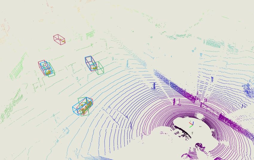
Published as a conference paper at ICLR 2022

               Training              Inference      T    Data Transformation         Outer Product     DE   Depth Estimator            D      Detector               B      Backbone

     RGB Data             RGB Data      DE       Depth Data    RGB Data        DE     Depth Data     RGB Data     DE     Depth Distribution       RGB Data               LiDAR Depth

                                                                     Pseudo-LiDAR       T               B       Image Feature                                Feature Guidance
        D                                                                                                                                                D                       D

                                        D                                      D                                   D
                                                                                                                                                             Response Guidance
      3D Box                                                                                                                                       3D Box                       3D Box
                                     3D Box                                3D Box                               3D Box

       (a)                             (b)                                     (c)                                 (d)                                              (e)

RGB-based method                                                    Depth-based method                                                                            Ours

                Figure 1: Comparison on the high-level paradigms of monocular 3D detectors.

estimator to provide depth cues. Specifically, they introduce a sub-network to estimate the depth
distribution and use it to enrich the RGB features. Although this model can be trained end-to-end
and achieves better performance, it still suffer from the low inference speed (630ms per image),
mainly caused by the depth estimator and the complicated network architecture. Note that the well-
designed monocular detectors, like Ma et al. (2021); Zhang et al. (2021b); Lu et al. (2021), only take
about 40ms per image.
In this paper, we aim to introduce the depth cues to the monocular 3D detectors without introducing
any extra cost in the inference phase. Inspired by the knowledge distillation (Hinton et al.), which
can transfer the learned knowledge from a well-trained CNN to another one without any changes
in the model design, we propose that the spatial cues may also be transferred by this way from the
LiDAR-based models. However, the main problem for this proposal is the difference of the feature
representations used in these two kinds of methods (2D images features vs. 3D voxel features). To
bridge this gap, we propose to project the LiDAR signals into the image plane and use the 2D CNN,
instead of the commonly used 3D CNN or point-wise CNN, to train a ‘image-version’ LiDAR-based
model. After this alignment, the knowledge distillation can be friendly applied to enrich the features
of our monocular detector.
Based on the above-mentioned motivation and strategy, we propose the distillation based monocular
3D detector (MonoDistill): We first train a teacher net using the projected LiDAR maps (used as the
ground truths of the depth estimator in previous works), and then train our monocular 3D detector
under the guidance of the teacher net. We argue that, compared with previous works, the proposed
method has the following two advantages: First, our method directly learn the spatial cues from
the teacher net, instead of the estimated depth maps. This design performs better by avoiding the
information loss in the proxy task. Second, our method does not change the network architecture of
the baseline model, and thus no extra computational cost is introduced.
Experimental results on the most commonly used KITTI benchmark, where we rank the 1st place
among all monocular based models by applying the proposed method on a simple baseline, demon-
strate the effectiveness of our approach. Besides, we also conduct extensive ablation studies to
present each design of our method in detail. More importantly, these experiments clearly illustrate
the improvements are achieved by the introduction of spatial cues, instead of other unaccountable
factors in CNN.

2    R ELATED W ORKS

3D detection from only monocular images. 3D detection from only monocular image data is
challenging due to the lack of reliable depth information. To alleviate this problem, lots of schol-
ars propose their solutions in different ways, including but not limited to network design (Roddick
et al., 2019; Brazil & Liu, 2019; Zhou et al., 2019; Liu et al., 2020; Luo et al., 2021), loss formu-
lation (Simonelli et al., 2019; Ma et al., 2021), 3D prior (Brazil & Liu, 2019), geometric constraint
(Mousavian et al., 2017; Qin et al., 2019; Li et al., 2019a; Chen et al., 2020b), or perspective mod-
eling (Zhang et al., 2021a; Lu et al., 2021; Shi et al., 2021).
Depth augmented monocular 3D detection. To provide the depth information to the 3D detectors,
several works choose to estimate the depth maps from RGB images. According to the usage of the

                                                                                        2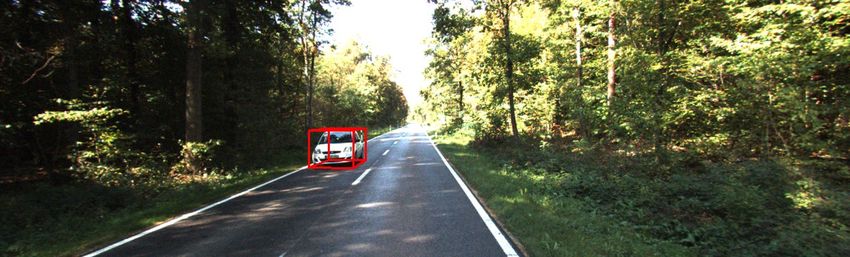
Published as a conference paper at ICLR 2022

      Figure 2: Visualization of the sparse LiDAR maps (left) and the dense LiDAR maps (right).

estimated depth maps, these methods can be briefly divided into three categories. The first class of
these methods use the estimated depth maps to augment the RGB images (Figure 1 (b)). In particular,
Xu & Chen (2018) propose three fusion strategies of the RGB images and depth maps, while Ding
et al. (2020) and Wang et al. (2021a) focus on how to enrich the RGB features with depth maps
in the latent feature space. Besides, Wang et al. (2019); Ma et al. (2019) propose another pipeline
(Figure 1 (c)): They back-project the depth maps into the 3D space, and then train a LiDAR-based
model and use the resulting data (pseudo-LiDAR signal) to predict the 3D boxes. This framework
shows promising performance, and lots of works (Weng & Kitani, 2019; Cai et al., 2020; Wang et al.,
2020a; Chu et al., 2021) are built on this solid foundation. Recently, Reading et al. (2021) propose
another way to leverage the depth cues for monocular 3D detection (Figure 1 (d)). Particularly, they
first estimate the depth distribution using a sub-network, and then use it to lift the 2D features into 3D
features, which is used to generate the final results. Compared with the previous two families, this
model can be trained in the end-to-end manner, avoiding the sub-optimal optimization. However,
a common disadvantage of these methods is that they inevitably increase the computational cost
while introducing depth information. Unlike these methods, our model chooses to learn the feature
representation under the guidance of depth maps, instead of integrating them. Accordingly, the
proposed model not only introduces rich depth cues but also maintains high efficiency.
Knowledge distillation. Knowledge distillation (KD) is initially proposed by Hinton et al. for
model compression, and the main idea of this mechanism is transferring the learned knowledge
from large CNN models to the small one. This strategy has been proved in many computer vision
tasks, such as 2D object detection (Dai et al., 2021; Chen et al., 2017; Gupta et al., 2016), semantic
semantic segmentation (Hou et al., 2020; Liu et al., 2019). However, few work explore it in monoc-
ular 3D detection. In this work, we design a KD-based paradigm to efficiently introduce depth cues
for monocular 3D detectors.
LIGA Stereo. We found a recent work LIGA Stereo (Guo et al., 2021) (submitted to arXiv on 18
Aug. 2021) discusses the application of KD for stereo 3D detection under the guidance of LiDAR
signals. Here we discuss the main differences of LIGA Stereo and our work. First, the tasks and
underlying data are different (monocular vs. stereo), which leads to different conclusions. For ex-
ample, Guo et al. (2021) concludes that using the predictions of teacher net as ‘soft label’ can not
bring benefits. However, our experimental results show the effectiveness of this design. Even more,
in our task, supervising the student net in the result space is more effective than feature space. Sec-
ond, they use an off-the-shelf LiDAR-based model to provide guidance to their model. However,
we project the LiDAR signals into image plane and use the resulting data to train the teacher net.
Except for the input data, the teacher net and student net are completely aligned, including network
architecture, hyper-parameters, and training schedule. Third, to ensure the consistent shape of fea-
tures, LIGA Stereo need to generate the cost volume from stereo images, which is time-consuming
(it need about 350ms to estimate 3D boxes from a KITTI image) and hard to achieve for monocular
images. In contrast, our method align the feature representations by adjusting the LiDAR-based
model, instead of the target model. This design makes our method more efficient (about 35ms per
image) and can generalize to all kinds of image-based models in theory.

3     M ETHOD

3.1     OVERVIEW

Figure 3 presents the framework of the proposed MonoDistill, which mainly has three components:
a monocular 3D detector, an aligned LiDAR-based detector, and several side branches which build

                                                    3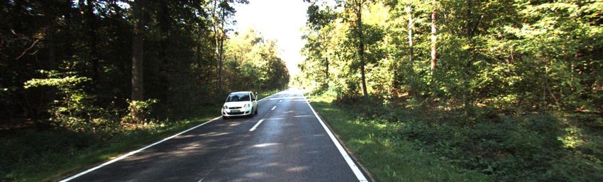
Published as a conference paper at ICLR 2022

                                                                                                                               Testing

                                                           …                       Detect head

      RGB Data                                                                                               3D detection result

                         Feature Fusion

                                                                                          Label diffusion
                 Feature Space                                                                                               Result Space

                            Scene-level Distillation   Object-level Distillation                            Object-level Distillation

                                                           …                       Detect head

   LiDAR Signal                                                                                             3D detection result

Figure 3: Illustration of the proposed MonoDistill. We first generate the ‘image-like’ LiDAR
maps from the LiDAR signals and then train a teacher model using an identical network to the
student model. Finally, we propose three distillation schemes to train the student model under the
guidance of the well-trained teacher net. In the inference phase, only the student net is used.

the bridge to provide guidance from the LiDAR-based detector to our monocular 3D detector. We
will introduce the how to build these parts one by one in the rest of this section.

3.2   BASELINE M ODEL

Student model. We use the one-stage monocular 3D detector MonoDLE (Ma et al., 2021) as our
baseline model. Particularly, this baseline model adopts DLA-34 (Yu et al., 2017) as the backbone
and uses several parallel heads to predict the required items for 3D object detection. Due to this
clean and compact design, this model achieves good performance with high efficiency. Besides, we
further normalize the confidence of each predicted object using the estimated depth uncertainty (see
Appendix A.1 for more details), which brings about 1 AP improvement * .
Teacher model. Existing LiDAR-based models are mainly based on the 3D CNN or point-wise
CNN. To align the gap between the feature representations of the monocular detector and the
LiDAR-based detector, we project the LiDAR points into the image plane to generate the sparse
depth map. Further, we also use the interpolation algorithm (Ku et al., 2018) to generate the dense
depth, and see Figure 2 for the visualization of generated data. Then, we use these ‘image-like
LiDAR maps’ to train a LiDAR-based detector using the identical network with our student model.

3.3   M ONO D ISTILL

In order to transfer the spatial cues from the well-trained teacher model to the student model, we de-
sign three complementary distillation schemes to provide additional guidance to the baseline model.
Scene-level distillation in the feature space. First, we think directly enforcing the image-based
model learns the feature representations of the LiDAR-based models is sub-optimal, caused by the
different modalities. The scene level knowledge can help the monocular 3D detectors build a high-
level understanding for the given image by encoding the relative relations of the features, keeping the
knowledge structure and alleviating the modality gap. Therefore, we train our student model under
the guidance of the high-level semantic features provided by the backbone of the teacher model. To
better model the structured cues, we choose to learn the affinity map (Hou et al., 2020) of high-level
    *
      Note that both the baseline model and the proposed method adopted the confidence normalization in the
following experiments for a fair comparison.

                                                                 4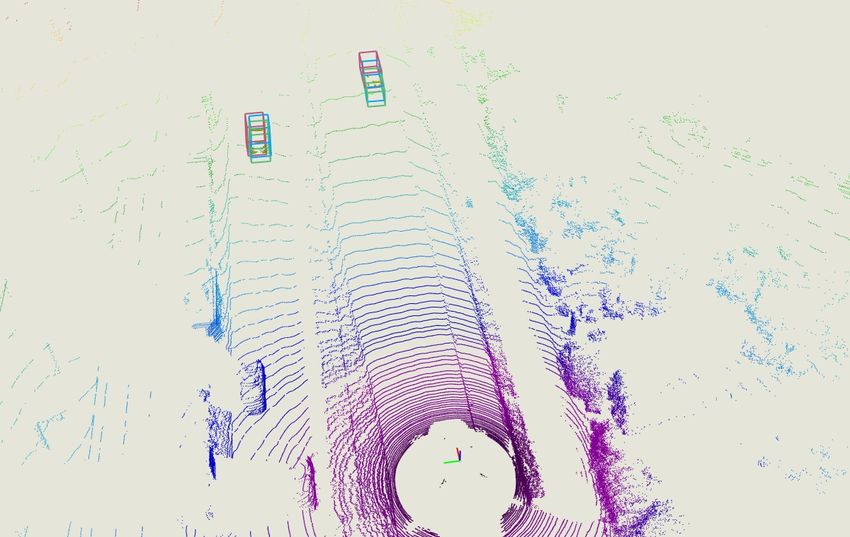
Published as a conference paper at ICLR 2022

features, instead of the features themselves. Specifically, we first generate the affinity map, which
encodes the similarity of each feature vector pair, for both the teacher and student network, and each
element Ai,j in this affinity map can be computed by:
                                                         fiT fj
                                         Ai,j =                       ,                              (1)
                                                  ||fi ||2 · ||fj ||2
where fj and fj denote the ith and jth feature vector. After that, we use the L1 norm to enforce the
student net to learn the structured information from the teacher net:
                                                K K
                                          1 XX t
                                Lsf =                  ||Ai,j − Asi,j ||1 ,                      (2)
                                        K × K i=1 j=1
where K is the number of the feature vectors. Note the computational/storage complexity is quadrat-
ically related to K. To reduce the cost, we group all features into several local regions and generate
the affinity map using the features of local regions. This makes the training of the proposed model
more efficient, and we did not observe any performance drop caused by this strategy.
Object-level distillation in the feature space. Second, except for the affinity map, directly using
the features from teacher net as guidance may also provide valuable cues to the student. However,
there is much noise in feature maps, since the background occupies most of the area and is less
informative. Distilling knowledge from these regions may make the network deviate from the right
optimization direction. To make the knowledge distillation more focused, limiting the distillation
area is necessary. Particularly, the regions in the ground-truth 2D bounding boxes are used for
knowledge transfer to mitigate the effects of noise. Specifically, given the feature maps of the
teacher model and student model {Ft , Fs }, our second distillation loss can be formulated as.
                                           1
                                  Lof =       ||Mof (Fs − Ft )||22 ,                            (3)
                                         Npos
where Mof is the mask generated from the center point and the size of 2D bounding box and Npos
is the number of valid feature vectors.
Object-level distillation in the result space. Third, similar to the traditional KD, we use the pre-
dictions from the teacher net as extra ‘soft label’ for the student net. Note that in this scheme, only
the predictions on the foreground region should be used, because the predictions on the background
region are usually false detection. As for the definition of the ‘foreground regions’, inspired by Cen-
terNet (Zhou et al., 2019), a simple baseline is regarding the center point as the foreground region.
Furtherly, we find that the quality of the predicted value of the teacher net near the center point is
good enough to guide the student net. Therefore, we generate a Gaussian-like mask (Tian et al.,
2019; Wang et al., 2021b) based on the position of the center point and the size of 2D bounding box
and the pixels whose response values surpass a predefined threshold are sampled, and then we train
these samples with equal weights (see Figure 4 for the visualization). After that, our third distillation
loss can be formulated as:
                                            XN
                                    Lor =       ||Mor (yks − ykt )||1 ,                               (4)
                                           k=1
where Mor is the mask which represents positive and negative samples, yk is the output of the k th
detection head and N is the number of detection heads.
Additional strategies. We further propose some strategies for our method. First, for the distillation
schemes in the feature space (i.e. Lsf and Lof ), we only perform them on the last three blocks of
the backbone. The main motivation of this strategy is: The first block usually is rich in the low-level
features (such as edges, textures, etc.). The expression forms of the low-level features for LiDAR
and image data may be completely different, and enforcing the student net to learn these features
in a modality-across manner may mislead it. Second, in order to better guide the student to learn
spatial-aware feature representations, we apply the attention based fusion module (FF in Table 1)
proposed by Chen et al. (2021b) in our distillation schemes in the feature space ( i.e. Lsf and Lof ).
Loss function. We train our model in an end-to-end manner using the following loss function:
                          L = Lsrc + λ1 · Lsf + λ2 · Lof + λ3 · Lor ,                        (5)
where Lsrc denotes the loss function used in the MonoDLE (Ma et al., 2021). λ1 , λ2 , λ3 are the
hyper-parameters to balance each loss. For the teacher net, only Lsrc is adopted.

                                                     5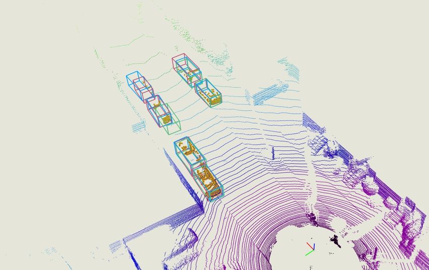
Published as a conference paper at ICLR 2022

Figure 4: Left: Regard the center point as the foreground region. Right: Generate foreground region
from the center point and the size of bounding box. Besides, the 2D bounding boxes are used as the
foreground region for Lof .

4     E XPERIMENTS
4.1   S ETUP

Dataset and metrics. We conduct our experiments on the KITTI (Geiger et al., 2012), which is
most commonly used dataset in 3D detection task. Specifically, this dataset provides 7,481 training
samples and 7,518 testing samples, and we further divide the training data into a train set (3,712
samples) and a validation set (3,769 samples), following prior works (Chen et al., 2015). Both 3D
detection and Bird’s Eye View (BEV) detection are evaluated using AP|R40 (Simonelli et al., 2019)
as metric. We report our final results on the testing set, while the ablation studies are conducted
on the validation set. Besides, we mainly focus on the Car category, while also present the perfor-
mances of Pedestrian and Cyclist in Appendix A.2 for reference.
Implementation. We provide the implementation details in Appendix A.1. Besides, our code will
be open-sourced for the reproducibility.

4.2   M AIN R ESULTS

Ablation studies. Table 1 shows the ablation studies of the proposed methods. Specifically, we
found that all three distillation schemes can improve the accuracy of the baseline model, and the
improvements of them are complementary. Besides, the feature fusion strategy can also boost the
accuracy. Compared with the baseline, our full model improves 3D detection performance by 3.34,
5.02, 2.98 and improve BEV performance by 5.16, 6.62, 3.87 on the moderate, easy and hard settings
respectively.

Table 1: Ablation studies on the KITTI validation set. SF, OF, and OR denote the scene-level dis-
tillation in feature space, the object-level distillation in feature space, and the object-level distillation
in result space, respectively. Besides, FF means the attention based feature fusion strategy.

                                               3D@IOU=0.7                 BEV@IOU=0.7
                SF     OF    OR      FF
                                           Mod. Easy Hard              Mod. Easy Hard
           a.                              15.13 19.29 12.78           20.24 26.47 18.29
           b.    X                         16.96 21.99 14.42           22.79 29.76 19.78
           c.          X                   16.85 21.76 14.36           22.30 28.93 19.31
           d.                 X            17.24 21.63 14.71           23.47 30.52 20.33
           e.    X     X                   17.33 22.34 14.63           22.90 30.02 19.84
           f.    X            X            17.70 22.59 15.17           23.59 31.07 20.46
           g.          X      X            17.98 22.58 15.26           23.76 30.98 20.52
           h.    X     X      X            18.24 23.82 15.49           25.06 32.66 21.88
           i.    X     X      X      X     18.47 24.31 15.76           25.40 33.09 22.16

Detailed design choice. We provide additional experiments in Table 2 for our method. First, as for
object-level distillation in the feature space, we investigate the different effects of applying distilla-
tion on the whole image and foreground regions. Due to the noise in the background, guiding the
foreground regions is more effective than the whole image, which improves the accuracy by 0.72 on

                                                     6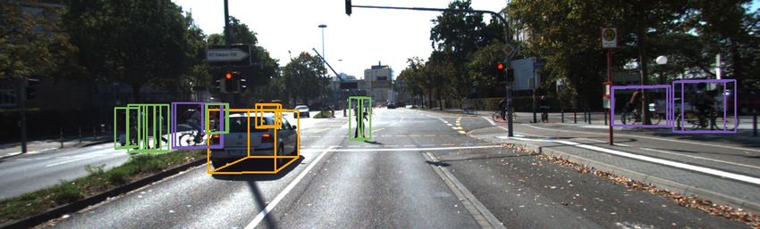
Published as a conference paper at ICLR 2022

the moderate settings in 3D detection. Second, as for object-level distillation in the result space, we
compare the different effects of point label and region label. It can be observed that the generated
region can significantly increase performance while guiding only in sparse point label brings limited
improvements. Our proposed label diffusion strategy can increase the number of positive samples
for supervision, thus improving performance.

Table 2: Evaluation on the KITTI validation set for detailed design choice. OF and OR represent
the object-level distillation in feature space and the object-level distillation in result space.

                                               3D@IOU=0.7                  BEV@IOU=0.7
           Guidance          Choice
                                           Mod. Easy Hard               Mod. Easy Hard
                              full         16.13 21.52 14.18            22.04 27.85 19.04
               OF
                          foreground       16.85 21.76 14.36            22.30 28.93 19.31
                          sparse label     15.51 20.58 13.70            21.47 27.16 18.60
              OR
                         diffused label    17.24 21.63 14.71            23.47 30.52 20.33

Comparison with state-of-the-art methods. Table 3 and Table 4 compare the proposed method
with other state-of-the-art methods on the KITTI test and validation sets. On the test set, the pro-
posed method outperforms existing methods in all metrics. We note that, compared with previous
best results, we can obtain 1.83, 0.50, 1.53 improvements on the moderate, easy and hard settings
in 3D detection. Furthermore, our method achieves more significant improvements in BEV detec-
tion, increasing upon the prior work by 2.51, 1.21, 2.46 on the moderate, easy and hard settings.
Moreover, compared with the depth-based methods, our method outperforms them in performance
by a margin and is superior to theirs in the inference speed. By contrast, our method only takes
40ms to process a KITTI image, tested on a single NVIDIA GTX 1080Ti, while the Fastest of the
depth-based methods (Ma et al., 2019; 2020; Ding et al., 2020; Wang et al., 2021a; Reading et al.,
2021) need 180ms. On the validation set, the proposed also performs best, both for the 0.7 IoU
threshold and 0.5 IoU threshold. Besides, we also present the performance of the baseline model to
better show the effectiveness of the proposed method. Note that we do not report the performances
of some depth-based methods (Ma et al., 2019; 2020; Ding et al., 2020; Wang et al., 2021a) due to
the data leakage problem * .

4.3   M ORE D ISCUSSIONS

What has the student model learned from the teacher model? To locate the source of improve-
ment, we use the items predicted from the baseline model to replace that from our full model, and
Table 5 summarizes the results of the cross-model evaluation. From these results, we can see that
the teacher model provides effective guidance to the location estimation (b→f), and improvement of
dimension part is also considerable (c→f). Relatively, the teacher model provides limited valuable
cues to the classification and orientation part. This phenomenon suggests the proposed methods
boost the performance of the baseline model mainly by introducing the spatial-related information,
which is consistent with our initial motivation. Besides, we also show the errors of depth estimation,
see Appendix A.3 for the results.
Is the effectiveness of our method related to the performance of the teacher model? An intuitive
conjecture is the student can learn more if the teacher network has better performance. To explore
this problem, we also use the sparse LiDAR maps to train a teacher net to provide guidance to the
student model (see Figure 2 for the comparison of the sparse and dense data). As shown in Table
6, the performance of the teacher model trained from the sparse LiDAR maps is largely behind by
that from dense LiDAR maps (drop to 22.05% from 42.45%, moderate setting), while both of them
provides comparable benefits to the student model. Therefore, for our task, the performance of the
teacher model is not directly related to the performance improvement, while the more critical factor
is whether the teacher network contains complementary information to the student network.
Do we need depth estimation as an intermediate task? As shown in Figure 1, most previous
methods choose to estimate the depth maps to provide depth information for monocular 3D detec-
tion (information flow: LiDAR data →estimated depth map→3D detector). Compared with this
    *
      these methods use the depth estimator pre-trained on the KITTI Depth, which overlaps with the validation
set of the KITTI 3D.

                                                      7
Published as a conference paper at ICLR 2022

Table 3: Comparison of state-of-the-art methods on the KITTI test set. Methods are ranked by
moderate setting. We highlight the best results in bold and the second place in underlined. Only
RGB images are required as input in the inference phase for all listed methods. *: need dense depth
maps or LiDAR signals for training. † : our baseline model without confidence normalization.

                                                  3D@IOU=0.7            BEV@IOU=0.7
  Method                                                                                    Runtime
                                             Mod. Easy     Hard     Mod. Easy    Hard
  M3D-RPN (Brazil & Liu, 2019)                9.71   14.76  7.42    13.67 21.02 10.23       160 ms
  SMOKE (Liu et al., 2020)                    9.76   14.03  7.84    14.49 20.83 12.75        30 ms
  MonoPair (Chen et al., 2020b)               9.99   13.04  8.65    14.83 19.28 12.89        60 ms
  RTM3D (Li et al., 2020)                    10.34 14.41    8.77    14.20 19.17 11.99        50 ms
  AM3D* (Ma et al., 2019)                    10.74 16.50    9.52    17.32 25.03 14.91       400 ms
  PatchNet* (Ma et al., 2020)                11.12 15.68 10.17      16.86 22.97 14.97       400 ms
  D4LCN* (Ding et al., 2020)                 11.72 16.65    9.51    16.02 22.51 12.55       200 ms
  MonoDLE† (Ma et al., 2021)                 12.26 17.23 10.29      18.89 24.79 16.00        40 ms
  MonoRUn* (Chen et al., 2021a)              12.30 19.65 10.58      17.34 27.94 15.24        70 ms
  GrooMeD-NMS (Kumar et al., 2021)           12.32 18.10    9.65    18.27 16.19 14.05       120 ms
  DDMP-3D* (Wang et al., 2021a)              12.78 19.71    9.80    17.89 28.08 13.44       180 ms
  CaDDN* (Reading et al., 2021)              13.41 19.17 11.46      18.91 27.94 17.19       630 ms
  MonoEF (Zhou et al., 2021)                 13.87 21.29 11.71      19.70 29.03 17.26        30 ms
  MonoFlex (Zhang et al., 2021b)             13.89 19.94 12.07      19.75 28.23 16.89        30 ms
  Autoshape (Liu et al., 2021)               14.17 22.47 11.36      20.08 30.66 15.59        50 ms
  GUPNet (Lu et al., 2021)                   14.20 20.11 11.77        -      -      -        35 ms
  Ours*                                      16.03 22.97 13.60      22.59 31.87 19.72        40 ms
  Improvements                               +1.83 +0.50 +1.53      +2.51 +1.21 +2.46          -

Table 4: Performance of the Car category on the KITTI validation set. We highlight the best
results in bold and the second place in underlined. † : our baseline model without confidence nor-
malization.

                          3D@IOU=0.7           BEV@IOU=0.7         3D@IOU=0.5          BEV@IOU=0.5
 Method
                      Mod. Easy Hard       Mod. Easy Hard      Mod. Easy Hard      Mod. Easy Hard
 M3D-RPN              11.07 14.53 8.65     15.62 20.85 11.88   35.94 48.53 28.59   39.60 53.35 31.76
 MonoPair             12.30 16.28 10.42    18.17 24.12 15.76   42.39 55.38 37.99   47.63 61.06 41.92
 MonoDLE†             13.66 17.45 11.68    19.33 24.97 17.01   43.42 55.41 37.81   46.87 60.73 41.89
 GrooMeD-NMS          14.32 19.67 11.27    19.75 27.38 15.92   41.07 55.62 32.89   44.98 61.83 36.29
 MonoRUn              14.65 20.02 12.61      -      -      -   43.39 59.71 38.44     -      -      -
 GUPNet               16.46 22.76 13.72    22.94 31.07 19.75   42.33 57.62 37.59   47.06 61.78 40.88
 MonoFlex             17.51 23.64 14.83      -      -      -     -     -      -      -      -      -
 Baseline             15.13 19.29 12.78    20.24 26.47 18.29   43.54 57.43 39.22   48.49 63.56 42.81
 Ours                 18.47 24.31 15.76    25.40 33.09 22.16   49.35 65.69 43.49   53.11 71.45 46.94

Table 5: Cross-model evaluation on the KITTI validation set. We extract each required item
(location, dimension, orientation, and confidence) from the baseline model (B) and the full model
(O), and evaluate them in a cross-model manner.

                                                  3D@IOU=0.7              BEV@IOU=0.7
               loc.     dim.   ori.   con.
                                              Mod. Easy Hard           Mod. Easy Hard
          a.    B        B      B      B      15.13 19.29 12.78        20.24 26.47 18.29
          b.    B        O      O      O      16.05 20.07 13.47        21.31 27.77 19.14
          c.    O        B      O      O      17.91 22.87 15.29        25.09 32.78 21.93
          d.    O        O      B      O      18.12 24.02 15.34        25.02 32.85 21.84
          e.    O        O      O      B      18.41 24.27 15.55        24.98 32.78 21.81
          f.    O        O      O      O      18.47 24.31 15.76        25.40 33.09 22.16

scheme, our method directly learns the depth cues from LiDAR-based methods (information flow:
LiDAR data→3D detector), avoiding the information loss in the depth estimation step. Here we
quantitatively show the information loss in depth estimation using a simple experiment. Specifi-
cally, we use DORN (Fu et al., 2018) (same as most previous depth augmented methods) to generate
the depth maps, and then use them to train the teacher net. Table 7 shows the results of this experi-

                                                     8
Published as a conference paper at ICLR 2022
Table 6: Performance of the student model under the guidance of different teacher models.
Metric is the AP|40 for the 3D detection task on the KITTI validation set. We also show the perfor-
mance improvements of the student model to the baseline model for better comparison.
Teacher Model Student Model Improvement
Mod. Easy Hard Mod. Easy Hard Mod. Easy Hard
sparse maps 22.05 31.67 18.72 18.07 23.61 15.36 +2.94 +4.32 +2.58
dense maps 42.57 58.06 37.07 18.47 24.31 15.76 +3.34 +5.02 +2.98
ment. Note that, compared with setting c, setting b’s teacher net is trained from a larger training set
(23,488 vs. 3,712) with ground-truth depth maps (ground truth depth maps vs. noisy depth maps).
Nevertheless, this scheme still lags behind our original method, which means that there is serious
information loss in monocular depth estimation (stereo image performs better, which is discussed in
Appendix A.4).
Table 7: Comparison of using depth estimation as intermediate task or not. Setting a. and c.
denote the baseline model and our full model. Setting b. uses the depth maps generated from DORN
(Fu et al., 2018) to train the teacher model. Experiments are conducted on the KITTI validation set.
3D@IOU=0.7 BEV@IOU=0.7 AOS@IOU=0.7 2D@IOU=0.7
Mod. Easy Hard Mod. Easy Hard Mod. Easy Hard Mod. Easy Hard
a. 15.13 19.29 12.78 20.24 26.47 18.29 90.95 97.46 83.02 92.18 98.37 85.05
b. 17.70 23.21 15.02 23.34 31.20 20.40 91.50 97.77 83.49 92.51 98.54 85.38
c. 18.47 24.31 15.76 25.40 33.09 22.16 91.67 97.88 83.59 92.71 98.58 85.56
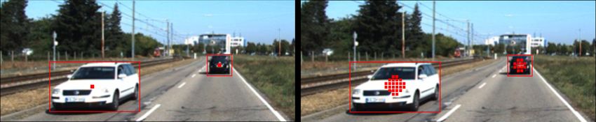
4.4 Q UALITATIVE R ESULTS
In Figure 5, we show the qualitative comparison of detection results. We can see that the proposed
method shows better localization accuracy than the baseline model. See Appendix A.7 for more
detailed qualitative results.
Figure 5: Qualitative results. We use green, blue and red boxes to denote the results from baseline,
our method, and ground truth. Besides, we use red circle to highlight the main differences.
5 C ONCLUSION
In this work, we propose the MonoDistill, which introduces spatial cues to the monocular 3D detec-
tor based on the knowledge distillation mechanism. Compared with previous schemes, which share
the same motivation, our method avoids any modifications on the target model and directly learns
the spatial features from the model rich in these features. This design makes the proposed method
perform well in both performance and efficiency. To show an all-around display of our model, ex-
tensive experiments are conducted on the KITTI dataset, where the proposed method ranks 1st at 25
FPS among all monocular 3D detectors.
9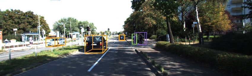
Published as a conference paper at ICLR 2022

ACKNOWLEDGEMENTS
This work was supported in part by the National Natual Science Foundation of China (NSFC) under
Grants No.61932020, 61976038, U1908210 and 61772108. Wanli Ouyang was supported by the
Australian Research Council Grant DP200103223, FT210100228, and Australian Medical Research
Future Fund MRFAI000085.

R EFERENCES
Garrick Brazil and Xiaoming Liu. M3d-rpn: Monocular 3d region proposal network for object
  detection. In ICCV, 2019.
Yingjie Cai, Buyu Li, Zeyu Jiao, Hongsheng Li, Xingyu Zeng, and Xiaogang Wang. Monocular 3d
  object detection with decoupled structured polygon estimation and height-guided depth estima-
  tion. In AAAI, 2020.
Jia-Ren Chang and Yong-Sheng Chen. Pyramid stereo matching network. In CVPR, 2018.
Guobin Chen, Wongun Choi, Xiang Yu, Tony X. Han, and Manmohan Chandraker. Learning effi-
  cient object detection models with knowledge distillation. In NeurIPS, 2017.
Hansheng Chen, Yuyao Huang, Wei Tian, Zhong Gao, and Lu Xiong. Monorun: Monocular 3d
  object detection by reconstruction and uncertainty propagation. In CVPR, 2021a.
Pengguang Chen, Shu Liu, Hengshuang Zhao, and Jiaya Jia. Distilling knowledge via knowledge
  review. In CVPR, 2021b.
Xiaozhi Chen, Kaustav Kundu, Yukun Zhu, Andrew G. Berneshawi, Huimin Ma, Sanja Fidler, and
  Raquel Urtasun. 3d object proposals for accurate object class detection. In NeurIPS, 2015.
Yilun Chen, Shu Liu, Xiaoyong Shen, and Jiaya Jia. DSGN: deep stereo geometry network for 3d
  object detection. In CVPR, 2020a.
Yongjian Chen, Lei Tai, Kai Sun, and Mingyang Li. Monopair: Monocular 3d object detection using
  pairwise spatial relationships. In CVPR, 2020b.
Xiaomeng Chu, Jiajun Deng, Yao Li, Zhenxun Yuan, Yanyong Zhang, Jianmin Ji, and Yu Zhang.
  Neighbor-vote: Improving monocular 3d object detection through neighbor distance voting. In
  ACM MM, 2021.
Xing Dai, Zeren Jiang, Zhao Wu, Yiping Bao, Zhicheng Wang, Si Liu, and Erjin Zhou. General
  instance distillation for object detection. In CVPR, 2021.
Mingyu Ding, Yuqi Huo, Hongwei Yi, Zhe Wang, Jianping Shi, Zhiwu Lu, and Ping Luo. Learning
 depth-guided convolutions for monocular 3d object detection. In CVPR, 2020.
Huan Fu, Mingming Gong, Chaohui Wang, Kayhan Batmanghelich, and Dacheng Tao. Deep ordinal
  regression network for monocular depth estimation. In CVPR, 2018.
Andreas Geiger, Philip Lenz, and Raquel Urtasun. Are we ready for autonomous driving? the KITTI
  vision benchmark suite. In CVPR, 2012.
Xiaoyang Guo, Shaoshuai Shi, Xiaogang Wang, and Hongsheng Li. Liga-stereo: Learning lidar
  geometry aware representations for stereo-based 3d detector. arXiv preprint arXiv:2108.08258,
  2021.
Saurabh Gupta, Judy Hoffman, and Jitendra Malik. Cross modal distillation for supervision transfer.
  In CVPR, 2016.
Geoffrey E. Hinton, Oriol Vinyals, and Jeffrey Dean. Distilling the knowledge in a neural network.
  CoRR, abs/1503.02531.
Yuenan Hou, Zheng Ma, Chunxiao Liu, Tak-Wai Hui, and Chen Change Loy. Inter-region affinity
  distillation for road marking segmentation. In CVPR, 2020.

                                                10
Published as a conference paper at ICLR 2022
Jason Ku, Ali Harakeh, and Steven L Waslander. In defense of classical image processing: Fast
depth completion on the cpu. In CRV, 2018.
Abhinav Kumar, Garrick Brazil, and Xiaoming Liu. Groomed-nms: Grouped mathematically dif-
ferentiable nms for monocular 3d object detection. In CVPR, 2021.
Buyu Li, Wanli Ouyang, Lu Sheng, Xingyu Zeng, and Xiaogang Wang. Gs3d: An efficient 3d object
detection framework for autonomous driving. In CVPR, 2019a.
Peiliang Li, Xiaozhi Chen, and Shaojie Shen. Stereo r-cnn based 3d object detection for autonomous
driving. In CVPR, 2019b.
Peixuan Li, Huaici Zhao, Pengfei Liu, and Feidao Cao. RTM3D: real-time monocular 3d detection
from object keypoints for autonomous driving. In ECCV, 2020.
Yifan Liu, Ke Chen, Chris Liu, Zengchang Qin, Zhenbo Luo, and Jingdong Wang. Structured
knowledge distillation for semantic segmentation. In CVPR, 2019.
Zechen Liu, Zizhang Wu, and Roland Tóth. SMOKE: single-stage monocular 3d object detection
via keypoint estimation. In CVPRW, 2020.
Zongdai Liu, Dingfu Zhou, Feixiang Lu, Jin Fang, and Liangjun Zhang. Autoshape: Real-time
shape-aware monocular 3d object detection. In ICCV, 2021.
Yan Lu, Xinzhu Ma, Lei Yang, Tianzhu Zhang, Yating Liu, Qi Chu, Junjie Yan, and Wanli Ouyang.
Geometry uncertainty projection network for monocular 3d object detection. In ICCV, 2021.
Shujie Luo, Hang Dai, Ling Shao, and Yong Ding. M3dssd: Monocular 3d single stage object
detector. In CVPR, 2021.
Xinzhu Ma, Zhihui Wang, Haojie Li, Pengbo Zhang, Wanli Ouyang, and Xin Fan. Accurate monoc-
ular 3d object detection via color-embedded 3d reconstruction for autonomous driving. In ICCV,
2019.
Xinzhu Ma, Shinan Liu, Zhiyi Xia, Hongwen Zhang, Xingyu Zeng, and Wanli Ouyang. Rethinking
pseudo-lidar representation. In ECCV, 2020.
Xinzhu Ma, Yinmin Zhang, Dan Xu, Dongzhan Zhou, Shuai Yi, Haojie Li, and Wanli Ouyang.
Delving into localization errors for monocular 3d object detection. In CVPR, 2021.
Arsalan Mousavian, Dragomir Anguelov, John Flynn, and Jana Kosecka. 3d bounding box estima-
tion using deep learning and geometry. In CVPR, 2017.
Charles R Qi, Wei Liu, Chenxia Wu, Hao Su, and Leonidas J Guibas. Frustum pointnets for 3d
object detection from rgb-d data. In CVPR, 2018.
Zengyi Qin, Jinglu Wang, and Yan Lu. Monogrnet: A geometric reasoning network for monocular
3d object localization. In AAAI, 2019.
Cody Reading, Ali Harakeh, Julia Chae, and Steven L. Waslander. Categorical depth distribution
network for monocular 3d object detection. In CVPR, 2021.
Thomas Roddick, Alex Kendall, and Roberto Cipolla. Orthographic feature transform for monocular
3d object detection. In BMVC, 2019.
Shaoshuai Shi, Xiaogang Wang, and Hongsheng Li. Pointrcnn: 3d object proposal generation and
detection from point cloud. In CVPR, 2019.
Shaoshuai Shi, Chaoxu Guo, Li Jiang, Zhe Wang, Jianping Shi, Xiaogang Wang, and Hongsheng
Li. PV-RCNN: point-voxel feature set abstraction for 3d object detection. In CVPR, 2020.
Xuepeng Shi, Qi Ye, Xiaozhi Chen, Chuangrong Chen, Zhixiang Chen, and Tae-Kyun Kim.
Geometry-based distance decomposition for monocular 3d object detection. In ICCV, 2021.
11Published as a conference paper at ICLR 2022
Andrea Simonelli, Samuel Rota Bulò, Lorenzo Porzi, Manuel Lopez-Antequera, and Peter
Kontschieder. Disentangling monocular 3d object detection. In CVPR, 2019.
Zhi Tian, Chunhua Shen, Hao Chen, and Tong He. FCOS: fully convolutional one-stage object
detection. In ICCV, 2019.
Li Wang, Liang Du, Xiaoqing Ye, Yanwei Fu, Guodong Guo, Xiangyang Xue, Jianfeng Feng, and
Li Zhang. Depth-conditioned dynamic message propagation for monocular 3d object detection.
In CVPR, 2021a.
Tai Wang, Xinge Zhu, Jiangmiao Pang, and Dahua Lin. FCOS3D: fully convolutional one-stage
monocular 3d object detection. CoRR, abs/2104.10956, 2021b.
Xinlong Wang, Wei Yin, Tao Kong, Yuning Jiang, Lei Li, and Chunhua Shen. Task-aware monocular
depth estimation for 3d object detection. In AAAI, 2020a.
Yan Wang, Wei-Lun Chao, Divyansh Garg, Bharath Hariharan, Mark E. Campbell, and Kilian Q.
Weinberger. Pseudo-lidar from visual depth estimation: Bridging the gap in 3d object detection
for autonomous driving. In CVPR, 2019.
Yan Wang, Xiangyu Chen, Yurong You, Li Erran Li, Bharath Hariharan, Mark Campbell, Kilian Q.
Weinberger, and Wei-Lun Chao. Train in germany, test in the usa: Making 3d object detectors
generalize. In CVPR, 2020b.
Xinshuo Weng and Kris Kitani. Monocular 3d object detection with pseudo-lidar point cloud. In
ICCVW, 2019.
Bin Xu and Zhenzhong Chen. Multi-level fusion based 3d object detection from monocular images.
In CVPR, 2018.
Jihan Yang, Shaoshuai Shi, Zhe Wang, Hongsheng Li, and Xiaojuan Qi. St3d: Self-training for
unsupervised domain adaptation on 3d object detection. In CVPR, June .
Yurong You, Yan Wang, Wei-Lun Chao, Divyansh Garg, Geoff Pleiss, Bharath Hariharan, Mark E.
Campbell, and Kilian Q. Weinberger. Pseudo-lidar++: Accurate depth for 3d object detection in
autonomous driving. In ICLR, 2020.
Fisher Yu, Dequan Wang, and Trevor Darrell. Deep layer aggregation. CoRR, abs/1707.06484,
2017.
Yinmin Zhang, Xinzhu Ma, Shuai Yi, Jun Hou, Zhihui Wang, Wanli Ouyang, and Dan Xu. Learning
geometry-guided depth via projective modeling for monocular 3d object detection. arXiv preprint
arXiv:2107.13931, 2021a.
Yunpeng Zhang, Jiwen Lu, and Jie Zhou. Objects are different: Flexible monocular 3d object
detection. In CVPR, 2021b.
Xingyi Zhou, Dequan Wang, and Philipp Krähenbühl. Objects as points. CoRR, abs/1904.07850,
2019.
Yunsong Zhou, Yuan He, Hongzi Zhu, Cheng Wang, Hongyang Li, and Qinhong Jiang. Monocular
3d object detection: An extrinsic parameter free approach. In CVPR, 2021.
12Published as a conference paper at ICLR 2022
A A PPENDIX
A.1 M ORE DETAILS OF THE BASELINE MODEL
Network architecture. The baseline network is extended from the anchor-free 2D object detection
framework, which consists of a feature extraction network and seven detection subheads. We employ
DLA-34 (Yu et al., 2017) without deformable convolutions as our backbone. The feature maps are
downsampled by 4 times and then we take the image features as input and use 3x3 convolution,
ReLU, and 1x1 convolution to output predictions for each detection head. Detection head branches
include three for 2D components and four for 3D components. Specifically, 2D detection heads
include heatmap, offset between the 2D key-point and the 2D box center, and size of 2D box. 3D
components include offset between the 2D key-point and the projected 3D object center, depth,
dimensions, and orientations. As for objective functions, we train the heatmap with focal loss. The
other loss items adopt L1 losses except for depth and orientation. The depth branch employs a
modified L1 loss with the assist of heteroscedastic aleatoric uncertainty. Common MultiBin loss is
used for the orientation branch. Besides, we propose a strategy to improve the accuracy of baseline.
Inspire by (Lu et al., 2021), estimated depth uncertainty can provide confidence for each projection
depth. Therefore, we normalize the confidence of each predicted box using depth uncertainty. In
this way, the score has capability of indicating the uncertainty of depth.
Training details. Our model is trained on 2 NVIDIA 1080Ti GPUs in an end-to-end manner for
150 epochs. We employ the common Adam optimizer with initial learning rate 1.25e−4 , and decay
it by ten times at 90 and 120 epochs. To stabilize the training process, we also applied the warm-up
strategy (5 epochs). As for data augmentations, only random random flip and center crop are applied.
Same as the common knowledge distillation scheme, we first train teacher network in advance, and
then fix the teacher network. As for student network, we simply train the detection model to give a
suitable initialization. We implemented our method using PyTorch. And our code is based on Ma
et al. (2021).
A.2 P EDESTRIAN /C YCLIST DETECTION .
Due to the small sizes, non-rigid structures, and limited training samples, the pedestrians and cyclists
are much more challenging to detect than cars. We first report the detection results on test set in Table
8. It can be seen that our proposed method is also competitive with current state-of-the-art methods
on the KITTI test set, which increases 0.69 AP on hard difficulty level of pedestrian category. Note
that, the accuracy of these difficult categories fluctuates greatly compared with Car detection due to
insufficient training samples (see Table 10 for the details). Due the access to the test server is limited,
we conduct more experiments for pedestrian/cyclist on the validation set for general conclusions
(we run the proposed method three times with different random seeds), and the experimental results
are summarized in Table 9. According to these results, we can find that the proposed method can
effectively boost the accuracy of the baseline model for pedestrian/cyclist detection.
Table 8: Performance of Pedestrian/Cyclist detection on the KITTI test set. We highlight the
best results in bold and the second place in underlined.
Pedestrian Cyclist
Method
Easy Mod. Hard Easy Mod. Hard
M3D-RPN 4.92 3.48 2.94 0.94 0.65 0.47
D4LCN 4.55 3.42 2.83 2.45 1.67 1.36
MonoPair 10.02 6.68 5.53 3.79 2.21 1.83
MonoFlex 9.43 6.31 5.26 4.17 2.35 2.04
MonoDLE 9.64 6.55 5.44 4.59 2.66 2.45
CaDDN 12.87 8.14 6.76 7.00 3.14 3.30
DDMP-3D 4.93 3.55 3.01 4.18 2.50 2.32
AutoShape 5.46 3.74 3.03 5.99 3.06 2.70
Ours 12.79 8.17 7.45 5.53 2.81 2.40
13Published as a conference paper at ICLR 2022
Table 9: Performance of Pedestrian/Cyclist detection on the KITTI validation set. Both 0.25
and 0.5 IoU thresholds are considered. We report the mean of several experiments for the proposed
methods. ± captures the standard deviation over random seeds.
3D@IoU=0.25 3D@IoU=0.5
Method
Easy Mod. Hard Easy Mod. Hard
Baseline 29.07±0.21 23.77±0.15 19.85±0.14 6.8±0.28 5.17±0.08 4.37±0.15
Pedestrian
Ours 32.09±0.71 25.53±0.55 21.15±0.79 8.95±1.26 6.84±0.81 5.32±0.75
Baseline 21.06±0.46 11.87±0.19 10.77±0.02 3.71±0.49 1.88±0.23 1.64±0.04
Cyclist
Ours 24.26±1.29 13.04±0.44 12.08±0.68 5.38±0.91 2.67±0.40 2.53±0.38
Table 10: Training samples of each category on the KITTI training set.
cars pedestrians cyclists
# instances 14,357 2,207 734
A.3 D EPTH E RROR A NALYSIS
As shown in Figure 6, we compare the depth error between baseline and our method. Specifically, we
project all valid samples of the Car category into the image plane to get the corresponding predicted
depth values. Then we fit the depth errors between ground truths and predictions as a linear function
by least square method. According to the experimental results, we can find that our proposed method
can boost the accuracy of depth estimation at different distances.
Figure 6: Errors of depth estimation. We show the errors of depth estimation as a function of the
depth (x-axis) for the baseline model (left) and our full model (right).
A.4 T HE E FFECTS OF S TEREO D EPTH
We also explored the changes in performance under the guidance of estimated stereo depth (Chang &
Chen, 2018), and show the results in Table 11. Stereo depth estimation exploits geometric constraints
in stereo images to obtain the absolute depth value through pixel-wise matching, which is more
accurate compared with monocular depth estimation. Therefore, under the guidance of stereo depth,
the model achieves almost the same accuracy as LiDAR signals guidance at 0.5 IoU threshold, and
there is only a small performance drop at 0.7 IoU threshold.
A.5 G ENERALIZATION OF THE PROPOSED METHOD
In the main paper, we introduced the proposed method based on MonoDLE (Ma et al., 2021). Here
we discuss the generalization ability of the proposed method.
Generalizing to other baseline models. To show the generalization ability of the proposed method,
we apply our method on another monocular detector GUPNet (Lu et al., 2021), which is a two-stage
detection method. Experimental results are shown in the Table 12. We can find that the proposed
14Published as a conference paper at ICLR 2022
Table 11: Effects of stereo depth estimation. Baseline denotes the baseline model without guid-
ance of teacher network. Stereo Depth and LiDAR Depth denote under the guidance of stereo depth
maps and LiDAR signals. Experiments are conducted on the KITTI validation set.
3D@IOU=0.7 BEV@IOU=0.7 3D@IOU=0.5 BEV@IOU=0.5
Mod. Easy Hard Mod. Easy Hard Mod. Easy Hard Mod. Easy Hard
Baseline 15.13 19.29 12.78 20.24 26.47 18.29 43.54 57.43 39.22 48.49 63.56 42.81
Stereo Depth 18.18 23.54 15.42 24.89 32.26 21.64 49.13 65.18 43.29 52.88 69.47 46.72
LiDAR Depth 18.47 24.31 15.76 25.40 33.09 22.16 49.35 65.69 43.49 53.11 71.45 46.94
method can also boosts the performances of GUPNet, which confirms the generalization of our
method.
Table 12: MonoDistill on GUPNet. Experiments are conducted on the KITTI validation set.
3D@IOU=0.7 3D@IOU=0.5
Easy Mod. Hard Easy Mod. Hard
GUPNet-Baseline 22.76 16.46 13.72 57.62 42.33 37.59
GUPNet-Ours 24.43 16.69 14.66 61.72 44.49 40.07
Generalizing to sparse LiDAR signals. We also explore the changes in performance under different
resolution of LiDAR signals. In particular, following Pseudo-LiDAR++ (You et al., 2020), we
generate the simulated 32-beam/16-beam LiDAR signals and use them to train our teacher model
(in the ‘sparse’ setting). We show the experimental results, based on MonoDLE, in the Table 13. We
can see that, although the improvement is slightly reduced due to the decrease of the resolution of
LiDAR signals, the proposed method significantly boost the performances of baseline model under
all setting.
Table 13: Effects of the resolution of LiDAR signals. Experiments are conducted on the KITTI
validation set.
3D@IOU=0.7 3D@IOU=0.5
Mod. Easy Hard Mod. Easy Hard
Baseline 19.29 15.13 12.78 43.54 57.43 39.22
Ours - 16-beam 22.49 17.66 15.08 49.39 65.45 43.60
Ours - 32-beam 23.24 17.71 15.19 49.41 65.61 43.46
Ours - 64-beam 23.61 18.07 15.36 49.67 65.97 43.74
More discussion. Besides, note that the camera parameters of the images on the KITTI test set are
different from these of the training/validation set, and the good performance on the test set suggests
the proposed method can also generalize to different camera parameters. However, generalizing
to the new scenes with different statistical characteristics is a hard task for existing 3D detectors
(Yang et al.; Wang et al., 2020b), including the image-based models and LiDAR-based models,
and deserves further investigation by future works. We also argue that the proposed method can
generalize to the new scenes better than other monocular models because ours model learns the
stronger features from the teacher net. These results and analysis will be included in the revised
version.
A.6 C OMPARISON WITH D IRECT D ENSE D EPTH S UPERVISION .
According to the ablation studies in the main paper, we can find that depth cues are the key factor
to affect the performance of the monocular 3D models. However, dense depth supervision in the
student model without KD may also introduce depth cues to the monocular 3D detectors. Here
we conduct the control experiment by adding a new depth estimation branch, which is supervised
by the dense LiDAR maps. Note that, this model is trained without KD. Table 14 compares the
performances of the baseline model, the new control experiment, and the proposed method. From
these results, we can get the following conclusions: (i) additional depth supervision can introduce
15Published as a conference paper at ICLR 2022
the spatial cues to the models, thereby improving the overall performance; (ii) the proposed KD-
based method significantly performs better than the baseline model and the new control experiment,
which demonstrates the effectiveness of our method.
Table 14: Comparison with direct dense depth supervision. Experiments are conducted on the
KITTI validation set.
3D@IOU=0.7 3D@IOU=0.5
Mod. Easy Hard Mod. Easy Hard
Baseline 15.13 19.29 12.78 43.54 57.43 39.22
Baseline + depth supv. 17.05 21.85 14.54 46.19 60.42 41.88
Ours 18.47 24.31 15.76 49.35 65.69 43.49
A.7 M ORE Q UALITATIVE R ESULTS
In Figure 7, we show more qualitative results on the KITTI dataset. We use orange box, green, and
purple boxes for cars, pedestrians, and cyclists, respectively. In Figure 8, we show comparison of
detection results in the 3D space. It can be found that our method can significantly improve the
accuracy of depth estimation compared with the baseline.
Figure 7: Qualitative results for multi-class 3D object detection. The boxes’ color of cars, pedestrian,
and cyclist are in orange, green, and purple, respectively.
16Published as a conference paper at ICLR 2022
Ground-truth
Baseline Depth: 36.28m
Ours
Depth: 45.95m
Depth: 37.96m
Figure 8: Qualitative results of our method for 3D space. The boxes’ color of ground truth, baseline,
and ours are in red, green, and blue, respectively.
17You can also read