Multi-Source Interactive Stair Attention for Remote Sensing Image Captioning
←
→
Page content transcription
If your browser does not render page correctly, please read the page content below
remote sensing
Article
Multi-Source Interactive Stair Attention for Remote Sensing
Image Captioning
Xiangrong Zhang                 , Yunpeng Li, Xin Wang, Feixiang Liu, Zhaoji Wu, Xina Cheng *                     and Licheng Jiao

                                         Key Laboratory of Intelligent Perception and Image Understanding of Ministry of Education, School of Artificial
                                         Intelligence, Xidian University, Xi’an 710071, China
                                         * Correspondence: xncheng@xidian.edu.cn

                                         Abstract: The aim of remote sensing image captioning (RSIC) is to describe a given remote sensing
                                         image (RSI) using coherent sentences. Most existing attention-based methods model the coherence
                                         through an LSTM-based decoder, which dynamically infers a word vector from preceding sentences.
                                         However, these methods are indirectly guided through the confusion of attentive regions, as (1) the
                                         weighted average in the attention mechanism distracts the word vector from capturing pertinent
                                         visual regions and (2) there are few constraints or rewards for learning long-range transitions. In
                                         this paper, we propose a multi-source interactive stair attention mechanism that separately models
                                         the semantics of preceding sentences and visual regions of interest. Specifically, the multi-source
                                         interaction takes previous semantic vectors as queries and applies an attention mechanism on
                                         regional features to acquire the next word vector, which reduces immediate hesitation by considering
                                         linguistics. The stair attention divides the attentive weights into three levels—that is, the core region,
                                         the surrounding region, and other regions—and all regions in the search scope are focused on
                                         differently. Then, a CIDEr-based reward reinforcement learning is devised, in order to enhance the
                                         quality of the generated sentences. Comprehensive experiments on widely used benchmarks (i.e., the
                                         Sydney-Captions, UCM-Captions, and RSICD data sets) demonstrate the superiority of the proposed
                                         model over state-of-the-art models, in terms of its coherence, while maintaining high accuracy.

                                         Keywords: remote sensing image captioning; cross-modal interaction; attention mechanism; semantic
Citation: Zhang, X.; Li, Y.; Wang, X.;
                                         information; encoder–decoder
Liu, F.; Wu, Z.; Cheng, X.; Jiao, L.
Multi-Source Interactive Stair
Attention for Remote Sensing Image
Captioning. Remote Sens. 2023, 15,
                                         1. Introduction
579. https://doi.org/10.3390/
rs15030579                                     Transforming vision into language has become a hot topic in the field of artificial
                                         intelligence in recent years. As a joint task of image understanding and language generation,
Academic Editor: Amin
                                         image captioning [1–4] has attracted the attention of more and more researchers. Specifically,
Beiranvand Pour
                                         the task of image captioning generates comprehensive and appropriate natural language,
Received: 12 November 2022               according to the content of the image. It is necessary to deeply study and understand
Revised: 5 January 2023                  the object, scene, and their relationship in the image for appropriate sentence generation.
Accepted: 11 January 2023                Due to the novelty and creativity of this task, image captioning has various application
Published: 18 January 2023               prospects, including human–computer interaction, blind assistant, battlefield environment
                                         analysis, and so on.
                                               With the rapid development of remote sensing technologies, the quantity and quality
                                         of remote sensing images (RSIs) have achieved great progress. Through these RSIs, we can
Copyright: © 2023 by the authors.
                                         observe the earth from an unprecedented perspective. Indeed, there are many differences
Licensee MDPI, Basel, Switzerland.
                                         between RSIs and natural images. First, RSIs usually contain large scale differences, causing
This article is an open access article
                                         the scene range and object size of RSIs to differ from that of natural images. Furthermore, the
distributed under the terms and
                                         modality of objects in RSIs is also very different from that in a natural image with overhead
conditions of the Creative Commons
                                         imaging. The rich information contained in an RSI can be further mined by introducing
Attribution (CC BY) license (https://
creativecommons.org/licenses/by/
                                         the task of image captioning into the RSI field, and the applications of the RSI can be
4.0/).
                                         further broadened. Many tasks, such as scene classification [5–7], object detection [8,9],

Remote Sens. 2023, 15, 579. https://doi.org/10.3390/rs15030579                                         https://www.mdpi.com/journal/remotesensing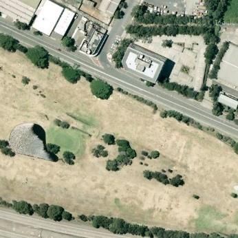
Remote Sens. 2023, 15, 579                                                                                             2 of 22

                             and semantic segmentation [10,11], focus on obtaining image category labels or object
                             locations and recognition. Remote sensing image captioning (RSIC) can extract more
                             ground feature information, attributes, and relationships in RSIs, in the form of natural
                             language to facilitate human understanding.

                             1.1. Motivation and Overview
                                    In order to determine the corresponding relationship between the generated words
                             and the image region, spatial attention mechanisms have been proposed and widely used
                             in previous studies [12,13]. Through the use of spatial attention mechanisms, such as hard
                             attention or soft attention [2], different regions of the image feature map can be given
                             different weights, such that the decoder can focus on the image regions related to the words
                             being generated. However, this correspondence leads to more attention being paid to the
                             location of the object, without full utilization of the semantic information of the object and
                             the text information of the generated sentence. In a convolutional neural network (CNN),
                             each convolution kernel encodes a pattern: a shallow convolution kernel encodes low-level
                             visual information, such as colors, edges, and corners, while a high-level convolution
                             kernel encodes high-level semantic information, such as the category of an object [14]. Each
                             channel of the high-level feature map represents a semantic attribute [4]. These semantic
                             attributes are not only important visual information in the image, but also important com-
                             ponents in the language description, which can help the model to understand the object
                             and its attributes more accurately. In addition, part of the generated sentence also contains
                             an understanding of the image. According to the generated words, some prepositions and
                             function words can be generated. On the other hand, most existing methods lack direct
                             supervision to guide the long-range sentence transition. The widely used maximum likeli-
                             hood estimation (i.e., cross-entropy) promotes accuracy in word prediction, but provides
                             little feedback for sentence generation in a given context. Reinforcement Learning (RL) has
                             achieved great success in natural image captioning (NIC) by addressing the gap between
                             training loss and evaluation metrics. Vaswani et al. [15] have presented an RL-based
                             self-critical sequence training (SCST) method, which improves the performance of image
                             captioning considerably. Through the effective combination of the above approaches, we
                             can enhance the understanding of the image content, thus obtaining more accurate sen-
                             tences. Inspired by the physiological structure of human retinal imaging [16], we re-think
                             the construction of spatial attention weighting. Being able to distinguish the color and
                             detail of objects better, the cone cells are mainly distributed near the fovea, and less around
                             the retina. This distribution pattern of the cone cells has an important impact on human
                             vision. In this line, a new spatial attention mechanism is constructed in this paper.
                                    Motivated by the above-mentioned reasons, we propose a multi-source interactive
                             stair attention (MSISAM) network. The proposed method mainly includes two serial
                             attention networks. One is a multi-source interactive attention (MSIAM) network. Different
                             from the spatial attention mechanism, focusing on the corresponding relationships between
                             words and image regions, it introduces the rich semantic information contained in the
                             channel dimension and the context information in the generated caption fragments. By
                             using a variety of information, the MSIAM network can selectively pay attention to the
                             feature maps output by CNNs. The other is the stair attention network, which is followed
                             by the MSIAM network, and in which the attentive weights are stair-like, according to the
                             degree of attention. Specifically, the calculated weights are shifted to the area of interest in
                             order to reduce the weight of the non-attention area. In addition, we devise a CIDEr-based
                             reward for RL-based training. This enhances the quality of long-range transitions and
                             trains the model more stably, improving the diversity of the generated sentences.

                             1.2. Contributions
                                  The core contributions of this paper can be summarized as follows:
                                  (1) A novel multi-source interactive attention network is proposed, in order to explore
                             the effect of semantic attribute information of RSIs and the context information of generated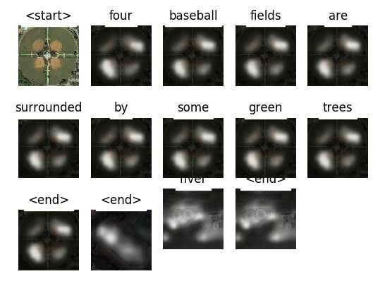
Remote Sens. 2023, 15, 579                                                                                             3 of 22

                             words to obtain complete sentences. This attention network not only focuses on the
                             relationship between the image region and the generated words, but also improves the
                             utilization of image semantics and sentence fragments. A variety of information works
                             together to allocate attention weights, in terms of space and channel, to build a semantic
                             communication bridge between image and text.
                                   (2) A cone cell heuristic stair attention network is designed to redistribute the existing
                             attention weights. The stair attention network highlights the most concerned image area,
                             further weakens the weights far away from the concerned area, and constructs a closer
                             mapping relationship between the image and text.
                                   (3) We further adopt a CIDEr-based reward to alleviate long-range transitions in the
                             process of sentence generation, which takes effect during RL training. The experimental
                             results show that our model is effective for the RSIC task.

                             1.3. Organization
                                  The remainder of this paper is organized as follows. In Section 2, some previous works
                             are briefly introduced. Section 3 presents our approach to the RSIC task. To validate the
                             proposed method, the experimental results are provided in Section 4. Finally, Section 5
                             briefly concludes the paper.

                             2. Related Work
                             2.1. Natural Image Captioning
                                   Many ideas and methods of the RSIC task come from the NIC task; therefore, it is
                             necessary to consider the research progress and research status in the NIC field. With the
                             publication of high-quality data sets, such as COCO, flickr8k, and flickr30k, the NIC task
                             also uses deep neural networks to achieve end-to-end sentence generation. Such end-to-end
                             implementations are commonly based on the encoder–decoder framework, which is the
                             most widely used frameworks in this field. These methods follow the same paradigm:
                             a CNN is used as an encoder to extract image features, and a recurrent neural network
                             (RNN) or long short-term memory (LSTM) network [17] is used as a decoder to generate a
                             description statement.
                                   Mao et al. [18] have proposed a multi-modal recurrent neural network (M-RNN)
                             which uses the encoder–decoder architecture, where the interaction of the CNN and RNN
                             occurs in the multi-modal layer to describe RSIs. Compared with RNN, LSTM solves the
                             problem of gradient vanishing while preserving the correlation of long-term sequences.
                             Vinyals et al. [1] have proposed a natural image description generator (NIC) model in
                             which the RNN was replaced by an LSTM, making the model more convenient for long
                             sentence processing. As the NIC model uses the image features generated by the encoder
                             at the initial time when the decoder generates words, the performance of the model is
                             restricted. To solve this problem, Xu et al. [2] have first introduced the attention mechanism
                             in the encoder–decoder framework, including hard and soft attention mechanisms, which
                             can help the model pay attention to different image regions at different times, then generate
                             different image feature vectors to guide the generation of words. Since then, many methods
                             based on attention mechanisms have been proposed.
                                   Lu et al. [19] have used an adaptive attention mechanism—the “visual sentinel”—which
                             helped the model to adaptively determine whether to focus on image features or text fea-
                             tures. When the research on spatial attention mechanisms was in full swing, Chen et al. [20]
                             proposed the SCA-CNN model, using both a spatial attention mechanism and a channel
                             attention mechanism in order to make full use of image channel information, which im-
                             proved the model’s perception and selection ability of semantic information in the channel
                             dimension. Anderson et al. [21] have defined the attention on image features extracted
                             from CNNs as top-down attention. Concretely, Faster R-CNN [22] was used to obtain
                             bottom-up attention features, which were combined with top-down attention features for
                             better performance. Research has shown that bottom-up attention also has an important
                             impact on human vision.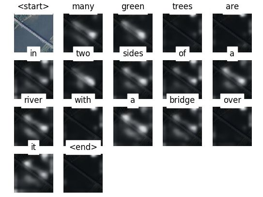
Remote Sens. 2023, 15, 579                                                                                             4 of 22

                                  In addition, the use of an attention mechanism on advanced semantic information can
                             also improve the ability of NIC models to describe key visual content. Wu et al. [23] have
                             studied the role of explicit high-level semantic concepts in the image content description.
                             First, the visual attributes in the image are extracted using a multi-label classification
                             network, following which they are introduced into the decoder to obtain better results.
                             As advanced image features, the importance of semantics or attributes in images has also
                             been discussed in [24–26]. The high-level attributes [27] have been directly employed for
                             NIC. The central spirit of this scheme aimed to strengthen the vision–language interaction
                             using a soft-switch pointer. Tian et al. [28] have proposed a controllable framework that
                             can generate captions grounded on related semantics and re-ranking sentences, which are
                             sorted by a sorting network. Zhang et al. [29] have proposed a transformer-based NIC
                             model based on the knowledge graph. The transformer applied multi-head attention to
                             explore the relation between the object features and corresponding semantic information.
                             Rennie et al. [30] have considered the problem that the evaluation metrics could not
                             correspond to the loss function in this task. Thus, an SCST RL-based method [15] has been
                             proposed to deal with the above problem.

                             2.2. Remote Sensing Image Captioning
                                   Research on RSIC started later than that of NIC. However, some achievements have
                             emerged by combining the characteristics of RSIs with the development of NIC. Shi et al. [31]
                             have proposed a template-based RSIC model. The full convolution network (FCN) first
                             obtains the object labels, and then a sentence template matches semantic information to
                             generate corresponding descriptions. Wang et al. [32] have proposed a retrieval-based
                             RSIC method, which selects the sentence closest to the input image in the representation
                             space as its description. The encoder–decoder structure is also popular in the field of RSIC.
                             Qu et al. [33] have explored the performance of a CNN + LSTM structure to generate
                             corresponding captions for RSIs, and disclosed results on two RSIC data sets (i.e., UCM-
                             captions and Sydney-captions). Many studies on attention-based RSIC models have recently
                             been performed; for example, Lu et al. [3] have explored the performance of an attention-
                             based encoder–decoder model, and disclosed results on the RSICD data set. The RSICD
                             further promotes the development of the RSIC task. The scene-level attention can produce
                             scene information for predicting the probability of each word vector. Li et al. [34] have
                             proposed a multi-level attention (MLA) including attention on image spatial domain,
                             attention on different texts, and attention for the interaction between vision and text,
                             which further enriched the connotation of attention mechanisms in RSIC task. Some
                             proposed RSIC models have aimed to achieve better representations of the input RSI, and
                             can alleviate the scale diversity problem, to some extent. For example, Ahmed et al. [35]
                             have introduced a multi-scale multi-interaction network for interacting multi-scale features
                             with a self-attention mechanism. The recurrent attention and semantic gate (RASG) [36]
                             utilizes dilated convolution filters with different dilation rates to learn multi-scale features
                             for numerous objects in RSIs. In the decoding phase, the multi-scale features are decoded
                             by the RASG, focusing on relevant semantic information. Zhao et al. [37] have produced
                             segmentation vectors in advance, such as hierarchical regions, in which the region vectors
                             are combined with the spatial attention to construct the sentence-level decoder. Unlike
                             multi-scale feature fusion, meta learning has been introduced by Yang et al. [38], where the
                             encoder inherited excellent performance by averaging several discrete task embeddings
                             clustered from other image libraries (i.e., natural images and RSIs for classification). Most
                             previous approaches have ignored the gap between linguistic consistency and image
                             content transition. Zhang et al. [4] have further generated a word-vector using an attribute-
                             based attention to guide the captioning process. The attribute features were trained to
                             highlight words that occurred in RSI content. Following this work, the label-attention
                             mechanism (LAM) [39] controlled the attention mechanism with scene labels obtained
                             by a pre-trained image classification network. Lu et al. [40] have followed the branch of
                             sound topic transition for the input RSI; but, differently, the semantics were separated from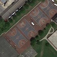
Remote Sens. 2023, 15, 579                                                                                         5 of 22

                             sound information to guide the attention mechanism. For the problem of over-fitting in
                             RS caption generation caused by CE loss, Li et al. [41] have improved the optimization
                             strategy using a designed truncated cross-entropy loss. Similarly, Chavhan et al. [42] have
                             used an actor dual-critic training strategy, which dynamically assesses the contribution of
                             the currently generated sentence or word. An RL-based training strategy was first explored
                             by Shen et al. [43], in the Variational Autoencoder and Reinforcement Learning-based Two-
                             stage Multi-task Learning Model (VRTMM). RL-based training uses evaluation metrics
                             (e.g., BLEU and CIDEr) as the reward, and VRTMM presented a higher accuracy.
                                   The usage of a learned attention is closely related to our formulation. In our case,
                             multi-source interaction is applied to high-level semantic understanding, rather than
                             internal activations. Furthermore, we employ a stair attention, instead of a common spatial
                             attention, thus imitating the human visual physiological structure.

                             3. Materials and Methods
                             3.1. Local Image Feature Processing
                                  The proposed model adopts the classical encoder–decoder architecture. The encoder
                             uses the classic CNN model, including VGG [44] and ResNet networks [45], and the output
                             of the last convolutional layer contains rich image information. Ideally, in the channel
                             dimension, each channel corresponds to the semantic information of a specific object, which
                             can help the model to identify the object. In terms of the spatial dimension, each position
                             corresponds to an area in the input RSI, which can help the model to determine where the
                             object is.
                                  We use a CNN as an encoder to extract image features, which can be written as follows:

                                                                        V = CNN ( I ),                                (1)
                             where I is the input RSI and CNN (·) denotes the convolutional neural network. In this
                             paper, four different CNNs (i.e., VGG16, VGG19, ResNet50, and ResNet101) are used as
                             encoders. Furthermore, V is the feature map of the output of the last convolutional layer of
                             the CNN, which can be expressed as:

                                                                   V = { v1 , v2 , . . . , v K },                     (2)

                             where K = W × H, vi ∈ RC represents the eigenvector of the ith (i = 1 ∼ K ) position of the
                             feature map, and W, H, and C represent the length, width, and channel of the feature map,
                             respectively. The mean value for V can be obtained as:

                                                                                    K
                                                                               1
                                                                         v=
                                                                               K   ∑ vi .                             (3)
                                                                                    i

                             3.2. Multi-Source Interactive Attention
                                  In the task of image captioning, the training samples provided are actually multi-
                             source, including information from both image and text. In addition, through processing
                             of the original training sample information, new features with clear meaning can be
                             constructed as auxiliary information, in order to improve the performance of the model.
                             Regarding the use of the training sample information, many current models are insufficient,
                             resulting in unsatisfactory performance. Therefore, it is meaningful to focus on how to
                             improve the utilization of sample information by using an attention mechanism.
                                  The above-mentioned feature map V can also be expressed in another form:

                                                                   U = { u1 , u2 , . . . , u C },                     (4)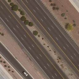
Remote Sens. 2023, 15, 579                                                                                             6 of 22

                             where ui ∈ R H ×W is the feature map of the ith channel. By calculating the mean value of
                             the feature map of each channel respectively, U can be represented as:

                                                                 U = { u1 , u2 , . . . , u C },                           (5)

                             where
                                                                                H W
                                                                      1
                                                              uk =
                                                                     H×W        ∑ ∑ uk (i, j),                            (6)
                                                                               i =1 j =1

                             where uk (i, j) is the value at position (i, j) of the kth channel feature uk of the feature map.
                                  As each channel is sensitive to a certain semantic object, the mean value of the channel
                             can also reflect the semantic feature of the corresponding object, to a certain extent. If the
                             mean value of each channel is collected, the semantic feature of an RSI can be represented
                             partly. Differing from the attribute attention [4], where the output of a fully connected layer
                             or softmax layer from a CNN was used to express the semantic features of an RSI, our model
                             uses the average of each channel to express the semantic features, thus greatly reducing
                             the amount of parameters, which can further improve the training speed of the model.
                             Meanwhile, in order to further utilize the channel dimension aggregation information, we
                             use an ordinary channel attention mechanism to weight different channels, improving the
                             response of clear and specific semantic objects in the image. In order to achieve the above
                             objectives and to learn the non-linear interactions among channels, the channel attention
                             weight β calculation formula is used, as follows:

                                                                    β=σ conv1×1 U ,                                        (7)

                             where β ∈ RC ; conv1×1 (·) denotes the 1 × 1 convolution operation; and σ (·) is the sigmoid
                             function, which can enhance the non-linear expression of network model. Slightly different
                             from SENet, we use 1 × 1 convolution, instead of the FC layer in SENet.
                                  The channel-level features F weighted by channel attention mechanism can be written
                             as follows:
                                                                 F = { f 1 , f 2 , . . . , f C },
                                                                                                                      (8)
                                                                 f i = β i ui .
                                 The Up-Down [21] has shown that the generated words can guide further word
                             generation. The word information at time t is given by the following formula:

                                                                        Tt = We Πt ,                                      (9)

                             where We denotes the word embedding matrix, and Πt is the one-hot coding of input words
                             at time t. Then, the multi-source attention weight, α1, can be constructed as:
                                                                             h                     i
                                                   α1tc = softmax(wαT ReLU( W f f c , unsq(WT Tt )
                                                                                                                (10)
                                                               +unsq( Wv v, Wh h1t ))),


                             where α1tc represents the multi-source attention weight weighted for the feature of channel
                                                             A             A             A                 A
                             c at time t; wα ∈ R A , W f ∈ R 2 ×C , WT ∈ R 2 ×E , Wv ∈ R 2 ×C , and Wh ∈ R 2 × M are trainable
                             parameters; A is the hidden layer dimension of the multi-source attention mechanism; M
                             is the output state h1t dimension of the multi-source LSTM; [, ] denotes the concatenation
                             operation on the corresponding dimension; and unsq(·) denotes expanding on the corre-
                             sponding dimension, in order to make the dimension of the concatenated object consistent.
                             The structure of multi-source interactive attention mechanism is depicted in Figure 1.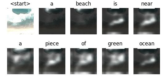
Remote Sens. 2023, 15, 579                                                                                             7 of 22

                                {u1 , u2 ,..., uC }                We Π t                   ht1                   v

                                   Global                          L&N                    L&N                    L&N
                                   pooling

                                                                  concate                             concate
                                 1×1 conv.

                                  Sigmoid
                                    β                                                                             L&N
                              Channel          Scale                add          ReLU             Dropout
                              Attention                                                                          Softmax
                                                      F
                                               L&N
                                                                                                            α1
                             Figure 1. The structure of MSIAM. The L&N layer performs the functions of Linearization and
                             Normalization. The Scale layer weights the input features.

                             3.3. Stair Attention
                                   The soft attention mechanism [2] processes information by treating the weighted
                             average of N input information as the output of the attention mechanism, while the
                             hard attention mechanism [2] randomly selects one of the N input information (i.e., the
                             information output is the one with the highest probability). The soft attention mechanism
                             may give more weight to multiple regions, resulting in more regions of interest and attention
                             confusion, while the hard attention mechanism only selects one information output, which
                             may cause great information loss and reduce the performance of the model. The above two
                             attention mechanisms are both extreme in information selection, so we design a transitional
                             attention mechanism to balance them.
                                   Inspired by the physiological structure of human retinal imaging, we re-framed the
                             approach to spatial attention weighting. There are two kinds of photoreceptors—cone
                             cells and rod cells—in the human retina. The cone cells are mainly distributed near the
                             central concave (fovea), but are less distributed around the retina. These cells are sensitive
                             to the color and details of objects. Retinal ganglion neurons are the main factors of image
                             resolution in human vision, and each cone cell can activate multiple retinal ganglion
                             neurons. Therefore, the concentrated distribution of cone cells plays an important role in
                             high-resolution visual observation. Some previous spatial attention mechanisms, such as
                             soft attention mechanisms, have imitated this distribution, but the weight distribution was
                             not very accurate. Based on the attention weights, these weights are regarded as reflecting
                             the distribution of cone cells; therefore, the area with the largest weight can be regarded
                             as the fovea, the cone cells around the fovea are reduced, and the cone cells far away
                             from the fovea are more sparser. In this way, the physiological structure of human vision
                             is imitated. As the distribution of attention weights is stair-like after classification, the
                             attention mechanism proposed in this section is named stair attention mechanism.
                                   After obtaining the multi-source interactive attention weights, we designed a stair
                             attention mechanism to redistribute the weights, as shown in Figure 2, which consists of
                             two modules: A data statistics module and a weight redistribution module.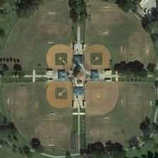
Remote Sens. 2023, 15, 579 8 of 22
α1max
Data Weight α2
α1 Statistics α1min Redistribution α
Module Module
( xi , yi )
Figure 2. The structure of MSISAM, which consists of two modules: A data statistics module and a
L
weight redistribution module. The symbol is the plus sign.
In the data statistics module, for multi-source attention weights α1i ∈ RW × H (i = 1 ∼ C),
the maximum weight value α1i max , the minimum weight value α1i min , and the coordinates
( xi , yi ) of the maximum weight value are determined as follows:
α1i max = MAX (α1i ),
α1i min = MI N (α1i ), (11)
( xi , yi ) = arg max(α1i ),
where MAX (·), MI N (·), and arg max(·) represent the maximum, minimum, and maxi-
mum position functions, respectively. The weight redistribution module is used to allocate
the weights of the output of the data statistics module. Taking α1i as an example, as a
two-dimensional matrix, the value ranges in the wide and high dimensions are 1 ∼ W and
1 ∼ H, respectively. The following three cases are based on the possible location of ( xi , yi ):
(1) ( xi , yi ) is located at the four corners of the feature map
∆1 = (1 − α1i max − (W × H − 1) × α1i min )/4,
α1i max + ∆1 w = xi , h = yi
(12)
α1i min + ∆1 w ∈ U ( xi , 3) [1, W ], h ∈ U (yi , 3) [1, H ],
T T
α2i (w, h) =
others
α1i min
In the above formula, α2i (w, h) represents the weight corresponding to the position
(w, h) of the ith channel of the stair attention weight α2, U (k, δ) represents the weight of the
T
δ-neighborhood of k, and is the union symbol (similarly below). The reason for dividing
∆1 by 4 is that there are only four elements in the α1i matrix in the 3-neighborhood of
( x i , y i ).
(2) ( xi , yi ) is on the edge of the feature map
∆2 = (1 − α1i max − (W × H − 1) × α1i min )/6,
α1i max + ∆2 w = xi , h = yi
(13)
α1i min + ∆2 w ∈ U ( xi , 3) [1, W ], h ∈ U (yi , 3) [1, H ],
T T
α2i (w, h) =
others
α1i min
There are six elements in the α1i matrix in the 3-neighborhood of ( xi , yi ).
(3) Other cases
∆3 = (1 − α1i max − (W × H − 1) × α1i min )/9,
α1i max + ∆3 w = xi , h = yi
(14)
α2i (w, h) = α1i min + ∆3 w ∈ U ( x i , 3) h ∈ U ( y i , 3),
others
α1i min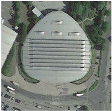
Remote Sens. 2023, 15, 579                                                                                                     9 of 22

                                    There are nine elements in the α1i matrix in the 3-neighborhood of ( xi , yi ). The reason
                             why 1 is subtracted in the above three cases is to ensure that the weight of all elements in
                             the feature map is 1.
                                    The stair attention weights for the above three cases are shown in Figure 3. The blue
                             region is the region with the lowest weight (i.e., the first stair). The pink area is the area
                             with the second lowest weight (i.e., the second stair). The red area is the highest weight area
                             (i.e., the third stair). The third stair is the area of the most concern, which can be compared
                             to the distribution of cone cells in the fovea of the human retina. The second stair is used
                             to simulate the distribution of cone cells around the fovea, where the attention is weaker,
                             but can assist the third stair. As the first stair is far away from the third stair, the attention
                             weight of the first stair is set to the lowest, and less resources are spent here.

                                       (1)                                    (2)                                    (3)
                             Figure 3. The weight distribution of stair attention in three cases. Different colors represent different
                             weight distributions.

                                 After the stair attention weight α2 is obtained, the final feature output after attention
                             weighting is obtained using the following formula:

                                                                                K
                                                                         vbt = ∑ αti vi ,
                                                                               i =1                                              (15)
                                                                         α = α1 + α2.

                             3.4. Captioning Model
                                  The decoder adopts the same strategy as the Up-Down [21], using a two-layer LSTM
                             architecture. The first LSTM, called multi-source LSTM, receives multi-source information.
                             The second LSTM is called language LSTM, and is responsible for generating descriptions.
                             In the following equation, superscript 1 is used to represent multi-source LSTM, while
                             superscript 2 represents language LSTM. The following formula is used to describe the
                             operation of the LSTM at time t:

                                                                     ht = LSTM( xt , ht−1 ),                                     (16)

                             where xt is the LSTM input vector and ht is the output vector. For convenience, the transfer
                             process of memory cells in LSTM is omitted here. The overall model framework is shown
                             in Figure 4.
                                  (1) Multi-source LSTM: As the first LSTM, the multi-source LSTM receives information
                             from the encoder, including the state information h2t−1 of the last step of the language LSTM,
                             the mean value v of the image feature representation, and the word information We Πt at
                             the current time step. The input vector can be expressed as:
                                                                       h               i
                                                                 xt1 = h2t−1 , v, We Πt .                               (17)

                                  (2) Language LSTM: The input of language LSTM includes the output of the stair
                             attention module and the output of the multi-source LSTM. It can be expressed by the
                             following formula:                      h      i
                                                                         xt2 = vbt , h1t ,                                       (18)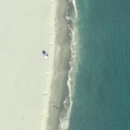
Remote Sens. 2023, 15, 579                                                                                                                 10 of 22

                             where y1:L represents the word sequence (y1 , . . . , y L ). At each time t, the conditional
                             probability of possible output words is as follows:

                                                        p(yt |y1:t−1 ) = softmax Wp h2t + b p ,                       (19)

                             where Wp ∈ R|Σ|× M and b p ∈ R|Σ| are learnable weights and biases. The probability
                             distribution on the complete output sequence is calculated through multiplication of the
                             conditional probability distribution:

                                                                                       L
                                                                   p(y1:L ) =        ∏ p(yt |y1:t−1 ).                                        (20)
                                                                                     t =1

                                                                                                                                      yt

                                                                         Reshape                                            Softmax
                                    CNN            {v1 , v2 ,..., vK }              {u1 , u2 ,..., uC }
                                                                                                                 ht2−1           ht2
                                                                Average
                                                                                                           vˆt             Language
                                                                                            ATT
                                                                                                                            LSTM
                                                                                                                                             ht2
                                                            v
                                                                                                                 ht1−1           ht1
                                                                                                                          Multi-source
                                                         We Π t                                                             LSTM             ht1

                                                                                                                              ht2−1

                             Figure 4. Overall framework of the proposed method. The CNN features of RSIs are first extracted. In
                             the decoder module, CNN features are modeled by the ATT block, which can be the designed MSIAM
                             or MSISAM. The multi-source LSTM and Language LSTM are used to preliminarily transform visual
                             information into semantic information.

                             3.5. Training Strategy
                                  During captioning training, the prediction of words at time t is conditioned on the
                             preceding words (y1:t−1 ). Given the annotated caption, the confidence of the prediction yt
                             is optimized by minimizing the negative log-likelihood over the generated words:

                                                                              T
                                                                         1
                                                             θ
                                                         lossCE =
                                                                         T   ∑ − log            pθt (yt |y1:t−1 , V ) ,                       (21)
                                                                             t =1

                             where θ denotes all learned parameters in the captioning model. Following previous
                             works [15], after a pre-training step using CE, we further optimize the sequence generation
                             through RL-based training. Specifically, we use the SCST [43] to estimate the linguistic
                             position of each semantic word, which is optimized for the CIDEr-D metric, with the reward
                             obtained under the inference model at training time:

                                                                  lossθRL = − Eω1:T ∼θ [r (ω1:T )],                                           (22)

                             where r is the CIDEr-D score of the sampled sentence   ω1:T . The gradient of lossθRL can be
                                                                       s

                             approximated by Equation (23), where r ω1:T    and r (ω̂1:T ) are the CIDEr rewards for the
                             random sampled sentence and the max sampled sentence, respectively.
                                                                     s                                s
                                                  ∇θ lossω
                                                         RL = −(r ( ω1:T ) − r ( ω̂1:T ))∇θ log( p ( ω1:T )).
                                                                                                  ω
                                                                                                                                              (23)
Remote Sens. 2023, 15, 579 11 of 22
4. Experiments and Analysis
4.1. Data Set and Setting
4.1.1. Data Set
In this paper, three public data sets are used to generate the descriptions for RSIs. The
details of the three data sets are provided in the following.
(1) RSICD [3]: All the images in RSICD data set are from Google Earth, and the size of
each image is 224 × 224 pixels. This data set contains 10,921 images, each of which is
manually labeled with five description statements. The RSICD data set is the largest
data set in the field of RSIC. There are 30 kinds of scenes in RSICD.
(2) UCM-Captions [33]: The UCM-Captions data set is based on the UC Merced (UCM)
land-use data set [46], which provides five description statements for each image.
This data set contains 2100 images of 21 types of features, including runways, farms,
and dense residential areas. There are 100 pictures in each class, and the size of each
picture is 256 × 256 pixels. All the images in this data set were captured from the large
image of the city area image from the national map of the U.S. Geological Survey.
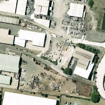
(3) Sydney-Captions [33]: The Sydney captions data set is based on the Sydney data
set [47], providing five description statements for each picture. This data set contains
613 images with 7 types of ground objects. The size of each image is 500 × 500 pixels.
4.1.2. Evaluation Metrics
Researchers have proposed several evaluation metrics to judge whether a description
generated by a machine is good or not. The most commonly used metrics for the RSIC
task include BLEU-n [48], METEOR [49], ROUGE_L [50], and CIDEr [51], which are used
as evaluation metrics to verify the effectiveness of a model. BLEU-n scores (n = 1, 2, 3,
or 4) represents the precision ratio by comparing the generated sentence with reference
sentences. Based on the harmonic mean of uniform precision and recall, the METEOR
score reflects the precision and recall ratio of the generated sentence. ROUGE_L captures
semantic quality by comparing scene graphs. The scene graph turns each component of
each tuple (i.e., object, object–attribute, subject–relationship–object) into a node. CIDEr
measures consistency between n-gram occurrences in generated and reference sentences,
where the consistency is weighted by n-gram saliency and rarity.
4.1.3. Training Details and Experimental Setup
In our experiments, VGG16 was used to extract appearance features, which is pre-
trained on the ImageNet data set [52]. Note that the size of the output feature maps from
the last layer of VGG16 is 14 × 14 × 512.
For three public data sets, the proportion of training, validation, and test sets in the
three data sets were 80%, 10%, and 10%, respectively. All RSIs were cropped to a size of
224 × 224 before being input to the model. In practice, all the experiments, including the
fine-tuning encoder process and the decoder training process, were carried out on a server
with an NVIDIA GeForce GTX 1080Ti. The hidden state size of the two LSTMs was 512.
Every word in the sentence was also represented as a 512-dimensional vector. Each selected
region was described with such a 512-dimensional feature vector. The initial learning rates
of the encoder and decoder were set to 1 × 10⁻⁵ and 5 × 10⁻⁴ , respectively. The mini-batch
size was 64. We set the maximum number of training iterations as 35 epochs. In order to
obtain better captions, the beam search algorithm was applied during the inference period,
with the number of beams equal to 3.
4.1.4. Compared Models
In order to evaluate our model, we compared it with several other state-of-the-art
approaches, which exploit either spatial or multi-task driven attention structures. We first
briefly review these methods in the following.Remote Sens. 2023, 15, 579 12 of 22
(1) SAT [3]: A architecture that adopts spatial attention to encode an RSI by capturing
reliable regional features.
(2) FC-Att/SM-Att [4]: In order to utilize the semantic information in the RSIs, this method
updates the attentive regions directly, as related to attribute features.
(3) Up-Down [21]: A captioning method that considers both visual perception and linguis-
tic knowledge learning to generate accurate descriptions.
(4) LAM [39]: A RSIC algorithm based on the scene classification task, which can generate
scene labels to better guide sentence generation.
(5) MLA [34]: This method utilizes a multi-level attention-based RSIC network, which
can capture the correspondence between each candidate word and image.
(6) Sound-a-a [40]: A novel attention mechanism, which uses the interaction of the knowl-
edge distillation from sound information to better understand the RSI scene.
(7) Struc-Att [37]: In order to better integrate irregular region information, a novel frame-
work with structured attention was proposed.
(8) Meta-ML [38]: This model is a multi-stage model for the RSIC task. The representation
for a given image is obtained using a pre-trained autoencoder module.
4.2. Evaluation Results and Analysis
We compared our proposed MSISAM with a series of state-of-the-art RSIC approaches
on three different data sets: Sydney-Captions, UCM-Captions, and RSICD. Specifically, for
the MSISAM model, we utilized the VGG16-based encoder for visual features and followed
reinforcement learning techniques in the training step. Tables 1–3 detail the performance
of our model and other attention-based models on the Sydney-Captions, UCM-Captions,
and RSICD data sets, respectively. It can be clearly seen that our model presented superior
performance over the compared models in almost all of the metrics. The best results of all
algorithms, using the same encoder, are marked in bold.
Table 1. Comparison of scores for our method and other state-of-the-art methods on the Sydney-
Captions data set [33].
Methods Bleu1 Bleu2 Bleu3 Bleu4 Meteor Rouge Cider
SAT[3] 0.7905 0.7020 0.6232 0.5477 0.3925 0.7206 2.2013
FC-Att [4] 0.8076 0.7160 0.6276 0.5544 0.4099 0.7114 2.2033
SM-Att [4] 0.8143 0.7351 0.6586 0.5806 0.4111 0.7195 2.3021
Up-Down [21] 0.8180 0.7484 0.6879 0.6305 0.3972 0.7270 2.6766
LAM [39] 0.7405 0.6550 0.5904 0.5304 0.3689 0.6814 2.3519
MLA [34] 0.8152 0.7444 0.6755 0.6139 0.4560 0.7062 1.9924
sound-a-a [40] 0.7484 0.6837 0.6310 0.5896 0.3623 0.6579 2.7281
Struc-Att [37] 0.7795 0.7019 0.6392 0.5861 0.3954 0.7299 2.3791
Meta-ML [38] 0.7958 0.7274 0.6638 0.6068 0.4247 0.7300 2.3987
Ours(SCST) 0.7643 0.6919 0.6283 0.5725 0.3946 0.7172 2.8122
Table 2. Comparison of scores for our method and other state-of-the-art methods on the UCM-
Captions data set [33].
Methods Bleu1 Bleu2 Bleu3 Bleu4 Meteor Rouge Cider
SAT [3] 0.7993 0.7355 0.6790 0.6244 0.4174 0.7441 3.0038
FC-Att [4] 0.8135 0.7502 0.6849 0.6352 0.4173 0.7504 2.9958
SM-Att [4] 0.8154 0.7575 0.6936 0.6458 0.4240 0.7632 3.1864
Up-Down [21] 0.8356 0.7748 0.7264 0.6833 0.4447 0.7967 3.3626
LAM [39] 0.8195 0.7764 0.7485 0.7161 0.4837 0.7908 3.6171
MLA [34] 0.8406 0.7803 0.7333 0.6916 0.5330 0.8196 3.1193
sound-a-a [40] 0.7093 0.6228 0.5393 0.4602 0.3121 0.5974 1.7477
Struc-Att [37] 0.8538 0.8035 0.7572 0.7149 0.4632 0.8141 3.3489
Meta-ML [38] 0.8714 0.8199 0.7769 0.7390 0.4956 0.8344 3.7823
Ours(SCST) 0.8727 0.8096 0.7551 0.7039 0.4652 0.8258 3.7129Remote Sens. 2023, 15, 579 13 of 22
Table 3. Comparison of scores for our method and other state-of-the-art methods on the RSICD data
set [3].
Methods Bleu1 Bleu2 Bleu3 Bleu4 Meteor Rouge Cider
SAT [3] 0.7336 0.6129 0.5190 0.4402 0.3549 0.6419 2.2486
FC-Att [4] 0.7459 0.6250 0.5338 0.4574 0.3395 0.6333 2.3664
SM-Att [4] 0.7571 0.6336 0.5385 0.4612 0.3513 0.6458 2.3563
Up-Down [21] 0.7679 0.6579 0.5699 0.4962 0.3534 0.6590 2.6022
LAM [39] 0.6753 0.5537 0.4686 0.4026 0.3254 0.5823 2.5850
MLA [34] 0.7725 0.6290 0.5328 0.4608 0.4471 0.6910 2.3637
sound-a-a [40] 0.6196 0.4819 0.3902 0.3195 0.2733 0.5143 1.6386
Struc-Att [37] 0.7016 0.5614 0.4648 0.3934 0.3291 0.5706 1.7031
Meta-ML [38] 0.6866 0.5679 0.4839 0.4196 0.3249 0.5882 2.5244
Ours(SCST) 0.7836 0.6679 0.5774 0.5042 0.3672 0.6730 2.8436
Quantitative Comparison: First, can be seen, the SAT obtained the lowest scores in
Tables 1–3, which was expected, as it only uses CNN–RNN without any modifications or
additions. It is worth mentioning that attribute-based attention mechanisms are utilized
in FC-Att, SM-Att, and LAM. Compared with SAT, adopting attribute-based attention in
the RSIC task improved the performance in all evaluation metrics (i.e., BLEU-n, METEOR,
ROUGE-L, and CIDEr). The LAM obtained a high CIDEr score on UCM-Captions and a low
BLEU-4 score on Sydney-Captions. This reveals that the UCM-Captions provides a larger
vocabulary than Sydney-Captions. However, for the RSICD data set, whose larger-scale
data and vocabulary may bring more difficulties in training the models, the improvement
was quite limited. The results of all models on the UCM-Captions data set are shown in
Table 2. The MLA model performed slightly better than our models in the METEOR and
ROUGE metrics; however, the performance of MLA on the Sydney-Captions and RSICD
data sets was not competitive.
To some extent, RSIC models with multi-task assistance have gradually been put
forward (i.e., Sound-a-a, Struc-Att, Meta-ML). Extra sound information is provided in
Sound-a-a, which led to performance improvements. On Sydney-Captions, the semantic
information was the most scarce. As shown in Table 1, Sound-a-a consistently outperformed
most methods in the CIDEr metric. In particular, the CIDEr score of Sound-a-a reached an
absolute improvement of 5.15% against the best competitor (Up-Down). Struc-Att takes
segmented irregular areas as visual inputs. The results of Struct-attention in Tables 1–3
also demonstrate that obtaining object structure features is useful. However, in some cases,
it presented worse performance (i.e., on RSICD). This is because the complex objects and
30 land categories in RSICD weakened the effectiveness of the segmentation block. To
extract image features considering the characteristics in RSIs, meta learning is applied
in Meta-ML, which could capture the strong grid features. In this way, as shown in
Tables 1–3, a significant improvement was obtained in all other metrics on the three data
sets. Thus, we consider that high-quality visual features provide convenient visual semantic
transformation.
In addition, we observed that the Up-Down model served as a strong baseline for
attention-based models. Up-Down utilizes double LSTM-based structures to trigger bottom-
up and top-down attention, leading to clear performance boosts. The results of the Up-
Down obtained showed better BLEU-n scores on the Sydney-Captions data set. Upon
adding the MSISAM in our model, the performance was further improved, compared to
using only CNN features and spatial attention. When we added the refinement module
(Ours*), we observed a slight degradation in the other evaluation metrics (BLUE-n, ME-
TEOR, and ROUGE-L). However, the CIDEr evaluation metric showed an improvement.
As can be seen from the results, the effectiveness of Ours* was confirmed, with improve-
ments of 13.56% (Sydney-Captions), 9.58% (UCM-Captions), and 24.14% (RSICD) in CIDEr,
when compared to the Up-Down model. Additionally, we note that our model obtainedRemote Sens. 2023, 15, 579 14 of 22
competitive performance, compared to other state-of-the-art approaches, surpassing them
in all evaluation metrics.
Qualitative Comparison: In Figure 5, examples of RSI content descriptions are shown,
from which it can be seen that the MSISAM captured more image details than the Up-
Down model. This phenomenon demonstrates that the attentive features extracted by
multi-source interaction with the stair attention mechanism can effectively enhance the
content description. The introduction of multi-source information made the generated
sentences more detailed. It is worth mentioning that the stair attention has the ability to
reallocate weights on the visual features dynamically at each time step.
GT: It is a peaceful beach with clear blue
waters.
Up-Down: It is a piece of farmland.
Ours*: This is a beach with blue sea and
white sands.
(a)
GT: There are two straight freeways in the
desert.
Up-Down: There are two straight freeways
with some plants besides them.
Ours*: There are two straight freeways
closed to each other with cars on the roads.
(b)
GT: There is a lawn with a industrial area
beside.
Up-Down: An industrial area with many
white buildings and a lawn beside.
Ours*: An industrial area with many white
buildings and some roads go through this
(c) area.
GT: Some marking lines on the runways
while some lawns beside.
Up-Down: There are some marking lines in
the runways while some lawns beside.
Ours*: There are some marking lines on the
runways while some lawns beside.
(d)
GT: Several large buildings and some green
trees are around a playground.
Up-Down: Some buildings and green trees
are in two sides of a railway station.
Ours*: A playground is surrounded by many
green trees and buildings.
(e)
GT: Four baseball fields are surrounded by
many green trees.
Up-Down: Two baseball fields are
surrounded by some green trees.
Ours*: Four baseball fields are surrounded
by some green trees.
(f)
Figure 5. Examples from: (a,b) UCM-Captions; (c,d) Sydney-Captions; and (e,f) RSICD. The output
sentences were generated by (1) one selected ground truth (GT) sentence; the (2) Up-Down model;
and (3) our proposed model without SCST (Ours*). The red words indicate mismatches with the
generated images, and the blue ones are precise words obtained with our model.
As shown in Figure 5a, the Up-Down model ignored the scenario information of “blue
sea” and “white sands”, while our proposed model identified the scene correctly in the
image, describing the color attributes of the sea and sand. For the scene “playground”, asRemote Sens. 2023, 15, 579 15 of 22
the main element of the image in Figure 5e, the “playground” was incorrectly described as
a “railway station” by the Up-Down model. MSISAM also improved the coherence of the
paragraph by explicitly modeling topic transition. As seen from Figure 5d, it organized
the relationship between “marking lines” and “runways” with “on”. At the same time,
Figure 5b shows that the MSISAM can describe small objects (i.e., “cars”) in the figure.
In addition, we found, from Figure 5f, that the sentences generated by Up-Down make
it difficult to obtain accurate quantitative information. Although the sentence reference
provides accurate quantitative knowledge, our model can tackle this problem and generated
an accurate caption (“four baseball fields”). It is worth noting that the proposed model
sometimes generated more appropriate sentences than the manually marked references: as
shown in Figure 5c, some “roads” in the “industrial area” are also described. The above
examples prove that the proposed model can further improve the ability to describe RSIs.
In addition, Figure 6 shows the image regions highlighted by the stair attention. For each
generated word, we visualized the attention weights for individual pixels, outlining the
region with the maximum attention weight in orange. From Figure 6, we can see that the
stair attention was able to locate the right objects, which enables it to accurately describe
objects in the input RSI. On the other hand, the visual weights were obviously higher when
our model predicted words related to objects (e.g., “baseball field” and “bridge”).
(a)
(b)
(c)
Figure 6. (a–c) Visualization of the stair attention map.
4.3. Ablation Experiments
Next, we conducted ablation analyses regarding the coupling of the proposed MSIAM,
MSISAM, and the combination of the latter with SCST. For convenience, we denote theseRemote Sens. 2023, 15, 579 16 of 22
models as A2, A3, and A4, respectively. Please note that all the ablation studies were
conducted based on the VGG16 encoder.
(1) Baseline (A1): The baseline [21] was formed by VGG16 combined with two LSTMs.
(2) MSIAM (A2): A2 denotes the enhanced model based on the Baseline, which utilizes
the RSI semantics from sentence fragments and visual features.
(3) MSISAM (A3): Integrating multi-source interaction with stair attention, A3 can high-
light the most concerned image areas.
(4) With SCST (A4): We trained the A3 model using the SCST and compared it with the
performance obtained by the CE.
Quantitative Comparison: For the A1, A2, and A3 models, the scores shown in
Tables 4–6 are under CE training, while those for the A4 model are with SCST train-
ing. Interestingly, ignoring the semantic information undermined the performance of
the Baseline, verifying our hypothesis that the interaction between linguistic and visual
information benefits cross-modal transition. A2 could function effectively, regarding the
integration of semantics from generated linguistics. However, the improvement was not
obvious for our A2 model combined with the designed channel attention, which learns
semantic vectors from visual features. From the results of A3, we utilized the stair attention
to construct a closer mapping relationship between images and texts, where A3 reduces
the difference among the distributions of semantic vector and attentive vector at different
time steps. As for diversity, the replacement-based reward enhanced the sentence-level
coherence. As can be seen in Tables 4–6, the use of the CIDEr metric led to great success, as
the increment-based reward promoted sentence-level accuracy. Thus, higher scores were
achieved when A3 was trained with SCST.
Table 4. Ablation performance of our designed model on the Sydney-Captions data set [33].
Methods Bleu1 Bleu2 Bleu3 Bleu4 Meteor Rouge Cider
A1 0.8180 0.7484 0.6879 0.6305 0.3972 0.7270 2.6766
A2 0.7995 0.7309 0.6697 0.6108 0.3983 0.7303 2.7167
A3 0.7918 0.7314 0.6838 0.6412 0.4079 0.7281 2.7485
A4 0.7643 0.6919 0.6283 0.5725 0.3946 0.7172 2.8122
Table 5. Ablation performance of our designed model on the UCM-Captions data set [33].
Methods Bleu1 Bleu2 Bleu3 Bleu4 Meteor Rouge Cider
A1 0.8356 0.7748 0.7264 0.6833 0.4447 0.7967 3.3626
A2 0.8347 0.7773 0.7337 0.6937 0.4495 0.7918 3.4341
A3 0.8500 0.7923 0.7438 0.6993 0.4573 0.8126 3.4698
A4 0.8727 0.8096 0.7551 0.7039 0.4652 0.8258 3.7129
Table 6. Ablation performance of our designed model on the RSICD data set [3].
Methods Bleu1 Bleu2 Bleu3 Bleu4 Meteor Rouge Cider
A1 0.7679 0.6579 0.5699 0.4962 0.3534 0.6590 2.6022
A2 0.7711 0.6645 0.5777 0.5048 0.3574 0.6674 2.7288
A3 0.7712 0.6636 0.5762 0.5020 0.3577 0.6664 2.6860
A4 0.7836 0.6679 0.5774 0.5042 0.3672 0.6730 2.8436
Qualitative Comparison : We show the descriptions generated by GT, the Baseline (A1),
MSIAM (A2), MSISAM (A3), and our full model (A4) in Figure 7. In Figure 7a, the word is
incorrectly included in captions (i.e., “stadium”) from Baseline, likely due to a stereotype.
Regarding such cases, A3 and A4, using the specific semantic heuristic, may determine the
correlation between a word’s most related regions. The “large white building” and “roads”
could be described in the scene by A3 and A4. Figure 7e is similar to Figure 7a, where
the “residential area” in the description is not correlated with the image topic. AnotherRemote Sens. 2023, 15, 579 17 of 22
noteworthy point is that the logical relationship between “buildings” and “park” was
disordered by A2. We extended the A2 with SCST to mine the sentence-level coherence for
boosting sentence generation (i.e., a “Some buildings are near a park with many green trees
and a pond”). As shown in Figure 7d, the caption generated by A4 was accurate, as well as
containing clear and coherent grammatical structure. The stair attention in A3 acts more
smoothly and allows for better control of the generated descriptions. In Figure 7c, where
the caption should include “two bridges”, this information was not captured by A1 or A2,
as inferring such content requires the amount of contextual and historical knowledge that
can be learned by A3 and A4.
GT: A playground is surrounded by white
buildings.
A1:Some buildings and green trees are
around a stadium.
A2:A playground is surrounded by a large
building.
A3:A large white building is near a
playground.
(a) A4:A playground is surrounded by a large
building and roads.
GT:Many buildings are in a dense
residential area.
A1:Many buildings and green trees are in
a school.
A2:Many buildings and green trees are in
a school.
A3:Many buildings and green trees are in
a school.
(b) A4:Many buildings and green trees are in
a school.
GT: Two bridges set up on the green rivers.
A1:A bridge is over a river with some
green trees in two sides.
A2:A bridge is over a river with some
green trees in two sides.
A3:There are some cars on the bridge.
A4:There are two roads across the river
with many green trees in two sides of it.
(c)
GT: Several buildings and green trees are
around a church.
A1:Some green trees are around a church.
A2:Some buildings and green trees are
around a church.
A3:Some buildings and green trees are
around a church.
A4:Several buildings and green trees are
(d) around a church.
GT: A lot of cars are parked in the park.
A1:Some buildings and green trees are in a
residential area.
A2:Some buildings and green trees are in a
park.
A3:Some buildings and green trees are
around a park.
A4:Some buildings are near a park with
(e)
many green trees and a pond.
GT: A large building is surrounded by some
green trees.
A1:Many buildings and green trees are in a
resort.
A2:Many buildings and green trees are in a
resort.
A3:Some storage tanks are near a river and
some green trees.
A4: Some storage tanks are near a river and
(f)
some green trees.
Figure 7. (a–f) Some typical examples on the RSICD test set. The GT sentences are human-annotated
sentences, while the other sentences are generated by the ablation models. The wrong words
generated by all models are indicated with red font; the green font words were generated by the
ablation models.Remote Sens. 2023, 15, 579 18 of 22
Despite the high quality of the captions for most of the RSIs, there were also some
examples of failures illustrated in Figure 7. Some objects in the generated caption were not
in the image. There were no schools in Figure 7b, but the word “school” was included in
all of the final descriptions. This may be due to the high frequency of some words in the
training data. Figure 7f shows another example of misrecognition. Many factors contribute
to this problem, such as the color or appearance of objects. The “resort” generated by A1
and A2 shared the same color with the roof of the “building”. In A3 and A4, the “storage
tanks” and “river” share the similar appearance with the roof of “building”. This is still an
open challenge in the RSIC field. Enabling models to predict the appropriate words through
the aid of external knowledge and common sense may help to alleviate this problem.
4.4. Parameter Analysis
In order to evaluate the influence of adopting different CNN features for the genera-
tion of sentences, experiments based on different CNN architectures were conducted. In
particular, VGG16, VGG19, ResNet50, and ResNet101 were adopted as encoders. Note that,
with the different CNN structures, the size of the output feature maps of the last layer of
the CNN network also differs. The size of the extracted features from the VGG networks
is 14 × 14 × 512, while the feature size was 7 × 7 × 2048 with the ResNet networks. In
Tables 7–9, we report the performance of Up-Down and our proposed models on the three
public data sets, respectively. The best results of the three different algorithms with the
same encoder are marked in bold.
Table 7. Comparison experiments on Sydney-Captions data set [33] based on different CNNs.
Methods Encoder Bleu1 Bleu2 Bleu3 Bleu4 Meteor Rouge Cider
Up-Down 0.8180 0.7484 0.6879 0.6305 0.3972 0.7270 2.6766
VGG16
MSISAM 0.7918 0.7314 0.6838 0.6412 0.4079 0.7281 2.7485
Up-Down 0.7945 0.7231 0.6673 0.6188 0.4109 0.7360 2.7449
VGG19
MSISAM 0.8251 0.7629 0.7078 0.6569 0.4185 0.7567 2.8334
Up-Down 0.7568 0.6745 0.6130 0.5602 0.3763 0.6929 2.4212
ResNet50
MSISAM 0.7921 0.7236 0.6647 0.6111 0.3914 0.7113 2.4501
Up-Down 0.7712 0.6990 0.6479 0.6043 0.4078 0.6950 2.4777
ResNet101
MSISAM 0.7821 0.7078 0.6528 0.6059 0.4078 0.7215 2.5882
Table 8. Comparison experiments on the UCM-Captions data set [33] based on different CNNs.
Methods Encoder Bleu1 Bleu2 Bleu3 Bleu4 Meteor Rouge Cider
Up-Down 0.8356 0.7748 0.7264 0.6833 0.4447 0.7967 3.3626
VGG16
MSISAM 0.8500 0.7923 0.7438 0.6993 0.4573 0.8126 3.4698
Up-Down 0.8317 0.7683 0.7205 0.6779 0.4457 0.7837 3.3408
VGG19
MSISAM 0.8469 0.7873 0.7373 0.6908 0.4530 0.8006 3.4375
Up-Down 0.8536 0.7968 0.7518 0.7122 0.4643 0.8111 3.5591
ResNet50
MSISAM 0.8621 0.8088 0.7640 0.7231 0.4684 0.8126 3.5774
Up-Down 0.8545 0.8001 0.7516 0.7067 0.4635 0.8147 3.4683
ResNet101
MSISAM 0.8562 0.8011 0.7531 0.7086 0.4652 0.8134 3.4686
Table 9. Comparison experiments on the RSICD data set [3] based on different CNNs.
Methods Encoder Bleu1 Bleu2 Bleu3 Bleu4 Meteor Rouge Cider
Up-Down 0.7679 0.6579 0.5699 0.4962 0.3534 0.6590 2.6022
VGG16
MSISAM 0.7712 0.6636 0.5762 0.5020 0.3577 0.6664 2.6860
Up-Down 0.7550 0.6383 0.5466 0.4697 0.3556 0.6533 2.5350
VGG19
MSISAM 0.7694 0.6587 0.5715 0.4986 0.3613 0.6629 2.6631
Up-Down 0.7687 0.6505 0.5577 0.4818 0.3565 0.6607 2.5924
ResNet50
MSISAM 0.7785 0.6631 0.5704 0.4929 0.3648 0.6665 2.6422
Up-Down 0.7685 0.6555 0.5667 0.4920 0.3561 0.6574 2.5601
ResNet101
MSISAM 0.7785 0.6694 0.5809 0.5072 0.3603 0.6692 2.7027You can also read