Multivariate Business Process Representation Learning utilizing Gramian Angular Fields and Convolutional Neural Networks
←
→
Page content transcription
If your browser does not render page correctly, please read the page content below
Multivariate Business Process Representation
                                          Learning utilizing Gramian Angular Fields and
                                                 Convolutional Neural Networks

                                                        Peter Pfeiffer, Johannes Lahann, and Peter Fettke

                                         German Research Center for Artificial Intelligence (DFKI) and Saarland University,
arXiv:2106.08027v1 [cs.LG] 15 Jun 2021

                                                                     Saarbrücken, Germany
                                                 {peter.pfeiffer, johannes.lahann, peter.fettke}@dfki.de

                                               Abstract. Learning meaningful representations of data is an important
                                               aspect of machine learning and has recently been successfully applied to
                                               many domains like language understanding or computer vision. Instead
                                               of training a model for one specific task, representation learning is about
                                               training a model to capture all useful information in the underlying data
                                               and make it accessible for a predictor. For predictive process analytics,
                                               it is essential to have all explanatory characteristics of a process instance
                                               available when making predictions about the future, as well as for clus-
                                               tering and anomaly detection. Due to the large variety of perspectives
                                               and types within business process data, generating a good representa-
                                               tion is a challenging task. In this paper, we propose a novel approach
                                               for representation learning of business process instances which can pro-
                                               cess and combine most perspectives in an event log. In conjunction with
                                               a self-supervised pre-training method, we show the capabilities of the
                                               approach through a visualization of the representation space and case
                                               retrieval. Furthermore, the pre-trained model is fine-tuned to multiple
                                               process prediction tasks and demonstrates its effectiveness in compari-
                                               son with existing approaches.

                                               Keywords: Predictive Process Analytics · Representation Learning ·
                                               Multi-view Learning

                                         1   Introduction
                                         Current machine-learning-based methods for predictive problems on business
                                         process data, e.g., neural-network-based methods like LSTMs or CNNs, achieve
                                         high accuracies in many tasks such as next activity prediction or remaining
                                         time prediction on many publicly available datasets [15]. In recent time, a large
                                         variety of new architectures for next step and outcome prediction have been
                                         proposed and evaluated [19,17,24]. These machine-learning-based methods are
                                         mostly task-specific and not generic, i.e., they are designed and tested on pre-
                                         dictive process analytics tasks like next step prediction, outcome prediction,
                                         anomaly detection, or clustering. Moreover, most of the proposed approaches
                                         process only one or a limited set of attributes including activity, resource [6] or
2 Pfeiffer et. al.
timestamp [23]. On one hand, predicting the next activity in an ongoing case
using the control-flow information is very similar to predicting the next word in a
sentence. On the other hand, data in an event log recorded from business process
executions is very rich in information. Usually, there are various attributes with
different types, scales, and granularity, which makes generating good representa-
tions containing all characteristics a difficult tasks. Characteristics of a process
instance that are embedded in the data attributes, can improve the performance
of predictive models [13]. For example, the next activity in a business process
can depend on multiple attributes in previous events and complex dependencies
between these attributes [2].
Inspired by recent research in the language modeling domain [5], we propose
and evaluate a novel and generic network architecture and training method –
the Multi-Perspective Process Network (MPPN) – which learns a meaningful,
multi-variate representation of a case in a general-purpose feature vector that
can be used for a variety of tasks. The research contributions of this paper is
threefold:
1. We introduce a novel neural-network-based architecture to process a flexible
number of process perspectives of a process instance that examines all of its
characteristics using gramian angular fields.
2. For this architecture, we propose an self-supervised pre-training method to
generate a feature-vector representation of a process instance that can be
fine-tuned to various tasks, thus making a contribution to representation
learning for predictive process analytics.
3. We show the effectiveness of this approach by analyzing the representation
space and performing an unsupervised case-retrieval task. Furthermore, we
fine-tune and compare the model on a variety of predictive process analytic
tasks such as next step and outcome prediction against existing approaches.
The structure of the remaining chapters unfolds as follows: Section 2 introduces
the reader to preliminary concepts. Section 3 discusses related work on the use
of machine learning in predictive process analytics and representation learning
for business process data. Section 4 and 5 present the proposed approach and
the evaluation on a variety of predictive process analytic tasks. Section 6 closes
the paper with a summary of the main contributions and findings as well as an
outline of future work.
2 Foundations
2.1 Business Process Event Log and Perspectives
Event logs contain records from process-aware information systems in a struc-
tured format. These recordings contain information about what activities have
been conducted by whom at what time as well as additional contextual data.
The following definitions will be used in later sections of the paper.MPPN 3 Definition 1 Event Log An event log is a tupel L = (E,
4      Pfeiffer et. al.

influence the prediction [2]. Usually, there are several attributes with different
types of data – categorical, numerical, and temporal ones. Within each type,
the dimensions, scales, and variabilities can be different. For instance, there can
be a numerical attribute cost ranging from [0, 1,000,000] and another one, e.g.,
discount that is in range [0, 30]. Temporal attributes also have different scales
(daily, weekly, monthly, etc.) and high variability. Categorical attributes often
vary in their dimensionality. While the activity has few different values, the re-
source, e.g., persons involved in a process, often has much more distinct values.
Some perspectives are very spare while others are rich. Furthermore, different
from event-related attributes, there are also case-related attributes. Some at-
tributes change their values only in certain events of a case, while others have
a different value for each event. This, in turn, means that perspectives have
different levels of granularity. When learning representations of cases, the multi-
variate, multi-scalar, and multi-granular nature of the data must be considered
and depicted.

3   Related Work

In [4], the authors introduced methods to learn representations of activities,
cases, and process models. They trained a model on the next step prediction task
to learn representations similar to obtaining embeddings for words, sentences,
and documents. Although they explained that other attributes besides activ-
ity are important, they only consider the control-flow perspective. Furthermore,
they did not include an extensive evaluation to elaborate on the effectiveness
of the proposed representations. Apart from that, representation learning is not
explicitly tackled in existing predictive analytic approaches. However, these ap-
proaches learn a representation alongside a specific prediction task. [6] was the
first to introduce neural networks to the field of process prediction. They applied
recurrent neural networks to next activity and remaining time prediction. They
trained separate neural networks considering the control-flow, resource, and time
perspectives. [23] examined the next step and remaining time prediction task.
They used an LSTM-based approach that optimized both tasks simultaneously
and elaborated on the effect of separated or shared LSTM network layers. [3]
elaborated three different LSTM architectures for predicting the next activity,
resource, and timestamp. In their first architecture, they used specialized layers
for each attribute to predict. The second version combines the categorical at-
tributes in a shares layer, while the third version shares categorical attributes
and the timestamp. In [17], the authors proposed an LSTM-based method that
can combine multiple attributes. In their model, the authors use embeddings for
each categorical attribute while non-categorical attributes are concatenated with
the categorical ones’ embedded representation. Other approaches for next step
prediction used different techniques such as decision trees (DT ) [9], autoencoder
(AE ) with n-grams [10], attention networks [12], CNNs [18] or generative adver-
sarial networks (GAN ) [24]. Similarly, CNNs [19], LSTMs [14] or autoencoder
[11] are used for outcome prediction. In order to detect anomalies in business
MPPN 5
Table 1: Overview of encoding techniques used in literature. duration: times-
tamps to duration after a certain timestamp, IMG: one or multiple perspectives
Π to a single or multiple matrices M h×w×c of size height × width × #channels.
Encoding Techniques for event attributes
Task Approach ML Method
Most common perspectives Other event log attributes
Πcontrol−f low Πresource Πtimestamp Categorical Numerical Temporal
[6] LSTM embedding - - - -
[23] LSTM one-hot - custom - - -
[10] AE + FF N-gram one-hot - one-hot as-is -
Next [9] DT integer integer
Step [18] CNN IMG - - -
Prediction [12] Attention one-hot one-hot - one-hot as-is -
[17] LSTM embedding embedding duration integer as-is duration
[3] LSTM embedding embedding duration - - -
[24] GAN one-hot - duration - - -
Outcome [19] CNN IMG - - -
Prediction [11] FF custom custom custom custom custom custom
[14] LSTM one-hot one-hot custom one-hot - -
Anomaly [16] LSTM integer integer - integer - -
Detection [20] Bayesian NN probability probability probability probability probability probability
All MPPN CNN IMG IMG IMG IMG IMG IMG
process data, LSTMs [16] or Bayesian neural networks [20] were applied. Ta-
ble 1 gives an overview of existing predictive approaches and categorizes them
by prediction task, examined perspective, encoding technique per perspective,
as well as used machine learning method. Also, it clarifies what information
is available to which model in what form. While all predictive approaches use
at least information from two perspectives, only a few approaches are able to
encode and process all types of attributes. We differentiated between the most
commonly used perspectives and other attribute types to delimit generic and
non-generic approaches. Only [17] used a generic encoding approach that can
process and represent all types of attributes. However, the approach is tailored
towards next step prediction and does not focus on the learned representation
within the model. Thus, we propose a generic multi-attribute representation
learning approach that is not tailored to a specific prediction task.
4 Multi-Perspective Process Network (MPPN)
The MPPN approach for representation learning is mainly built on two concepts
– graphical event log encoding and neural-network-based processing. The first
part is to encode the perspectives of interest Π̂ in the event log L uniformly
as 2D images by transforming them to distinct gramian angular fields (GAF)
– no matter if the perspective contains categorical, numerical or temporal in-
formation. The second part is a convolutional neural network architecture and
training method that learns representations of cases using the GAF-encoded per-
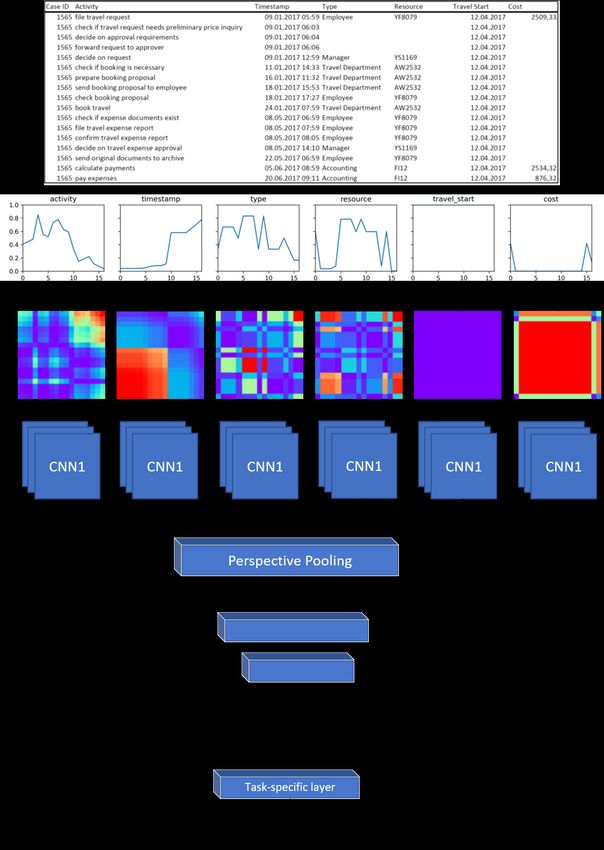
spectives. Figure 1 shows the architecture and processing pipeline of the MPPN
approach. In this example, the six perspectives of interest Π̂ = {Πcontrol−f low ,
Πtimestamp , Πtype , Πresource , Πtravel start Πcost of the case with case-id 1565 are
first encoded as six individual GAFs, which can then be processed by the MPPN.6 Pfeiffer et. al. Fig. 1: Architecture and processing pipeline of MPPN using a case from the MobIS event log [7]. CNN1 extracts the features of each perspective Π̂ which are combined in the perspective pooling layer. The combined features capture all characteristics of interest of a particular case. The forwards pass in MPPN of a single case c is as follows: For each GAF-encoded perspective, CNN1 extracts a feature vector that is pooled before being passed to NN2. NN2 then takes the pooled features from all perspectives, processes them, and produces a single feature vector F V . This two-stage architecture allows CNN1 to focus on the features within each per- spective while NN2 captures and models the dependencies between perspectives. By transforming all perspectives uniformly to GAFs, all attributes lie within the same range, no matter what scale or variability they had before. At the same time, NN2 can learn what features from what perspectives are important. Unlike RNN-based models, MPPN consumes the whole case at once instead of being
MPPN          7

fed with cases event by event.
Inspired by multi-view learning, e.g., Multi-View Convolutional Neural Net-
works (MVCNN) for 3D object detection using 2D renderings [22], the Multi-
Perspective Process Network creates a feature vector F V for a case using the
GAF-encoded perspectives. Analogous to using multiple renders from different
views to represent 3D structures, we use different perspectives of a process to
represent a case. Another important aspect of MPPN is its ability to be used for
several tasks instead of being task-specific. This is achieved by an self-supervised
pre-training phase, as also done in[10], that learns a representation in the form
of a feature vector F V . Afterwards, a task-specific layer can be added to the pre-
trained model allowing to fine-tune the model on different tasks. The learned
representation F V thus serves as the basis for any downstream task.

4.1   Graphical Representation of Event Log Data

In order to encode all types of attributes into a single representation in a generic
way, we decided to choose a graphical encoding instead of the methods used in
related work shown in table 1. We see a strong similarity in the characteristics
of time-series and a single perspective of a process case. Furthermore, all types
of attributes in a case can easily be transformed to time-series. For this reason,
we treat the perspectives Π̂ as multivariate time series. A naive way to get
a both machine-readable and visualizable representations of perspectives Π is
to represent and plot them as time series. Thus, each value of a perspective is
encoded as a real number and visualized in a 2D representation. The y-coordinate
corresponds to the value v, and the x-coordinate to t. In figure 1, one can see
the 6 perspectives Π̂ of case 1565 encoded and plotted as 6 distinct time series.
Although this representation is a nice visualization for humans, presenting the
perspectives Π as a time series plot is a very naive way. Such a plot is very
sparse, i.e., most of the plot is empty with just a fine line drawn, containing only
little information for convolutional neural networks.
     Gramian angular fields (GAF), originally proposed for time-series classifica-
tion, transform sequential data to 2D images, which contain more information
for machine learning methods as time-series plots [26]. For a sequence hv1 , ..., vn i,
a gramian angular field is a matrix of size n × n where each entry is the cosine
of the sum of two polar coordinates in time – the polar coordinate of vi plus
vj . This projection is bijective and preserves temporal relations. To transform
event log data, i.e., all perspectives Π̂ of categorical, numerical, and temporal
event log attributes and case attributes into gramian angular fields, they must
be treated and transformed to distinct sequences of numerical values. In order
to get numerical sequences from each type, the following transformations and
encodings are performed. Other types of attributes can also be used (e.g., textual
data) if they are encoded as numerical sequences.

 1. For categorical attributes ai , we applied an integer encoding integer : Vi →
    int where int ∈ [0, 1, 2, .., |Vi | − 1].
8 Pfeiffer et. al.
2. Timestamps are transformed into the duration in seconds from the earliest
timestamp.
3. Numerical attributes are used unchanged.
Case attributes are first duplicated to the case length before being encoded in
the same way as event attributes. Once encoded as numerical sequences, each
perspective can easily be encoded as a gramian angular field after scaling them
to a [-1, 1] range. To ensure equal size images where characteristics are equally
represented, the sequences are adjusted to equal length, either by padding or
truncating. This results in distinct GAF-representations for each perspective Π̂
of a case as shown in figure 1.
By using graphical encodings we can transform attributes of different types to
images and use state-of-the-art image processing neural networks. This way we
avoid building networks that process cases with customized architectures for
specific attribute types as well as the complexity of training embeddings.
4.2 Architecture
The MPPN architecture consists of three parts as shown in figure 1: CNN1 for
feature extraction, NN2 for modeling dependencies and relations between per-
spectives, and one or multiple task-specific layers called HEAD. Between CNN1
and NN2, a pooling layer combines the features produced by CNN1 for each
GAF-encoded perspective to a single vector. The weights in CNN1 are shared
between all perspectives, i.e. the same CNN1 is applied on all perspectives.
For CNN1, we use Alexnet [8]. However, as gramian angular fields are different
from natural images, pre-training CNN1 on GAFs significantly reduces the later
training time. NN2 is a fully-connected neural network. Together, CNN1 and
NN2 form the model used for representation learning that produces F V . F V can
either be used directly or by any other task-specific layer; e.g., a fully-connected
HEAD with softmax for next step prediction or a HEAD for remaining time
prediction.
4.3 Training Method
One integral part of MPPN is its ability to learn representations of all perspec-
tives Π̂ of cases in an event log. In order to obtain good feature vectors F V , one
must ensure that all relevant characteristics are fully captured in the model. We
distinguish three stages of training that should be performed successively.
Pre-Training CNN1 on GAFs As GAFs are very different from natural
images, pre-trained CNNs like Alexnet need to be fine-tuned. While lower-level
features like edges and corners are present in GAFs too, higher-level features
differ. In order to make the MPPN sensitive to GAF-specific feature, we fine-
tuned the CNN1 once by classifying cases according to their variant. This task
has been chosen as the process variant is always directly derivable from theMPPN 9 sequence of events and the model can focus on learning features from the single GAF-encoded perspective. All relevant information for this task is entailed in the GAF image which is what we want the model to focus on. However, many other tasks are also possible. In detail, we build a MPPN with a pre-trained Alexnet consuming only Πcontrol−f low and predicting the variant on the MobIS dataset. For each case c the whole sequence of activity was used as input and the variant used as the target. Afterwards, the weights of CNN1 are saved on disk and can be used on any dataset, any perspective, and any task for MPPN in the future. Representation Learning To obtain meaningful feature vectors F V of busi- ness process cases, MPPN must be trained to hold all characteristics of a case in it. One can train MPPN on next step prediction tasks, e.g., to predict the next activity in an ongoing case given Π̂. This works fine, but the model will learn the relation in the data, which are important for the next activity. This leads to a feature vector F V that by design holds features that are important to predict the next activity. Attributes that do not have relevance for the next activity will be less present in F V . To obtain more generic feature vectors of cases, a self-supervised multi-task next event prediction training method is applied that trains the network to predict ai (et+1 ) for each attribute in Π̂. For this task, the MPPN architecture is ex- tended by small networks HEADai – one for each attribute ai to predict. Each HEAD is a task-specific layer that consumes F V and predicts ai (et+1 ). During representation learning, the task’s criterion is to minimize the sum of all losses of all predictions, measured as mean absolute error (for numerical and tempo- ral attributes) and cross-entropy (for categorical attributes). During training, all HEADs are trained in parallel and in conjunction with the rest of MPPN. Thereby, the MPPN and especially NN2 learns to focus on important features in all perspectives Π̂ and produces a F V that holds information relevant for the attributes in the next event. Using this method, a representation can be learned without the need for manual labeled data. However, depending on the final task to be solved, other training methods are also possible. As long as all relevant characteristics of the case are enclosed in F V , any training method is appropriate. We chose the multi-task next event prediction task as it allows the model to incorporate all attributes for each prediction. While making predictions for each attribute the model is forced to not drop relevant characteristics of a case. Afterwards, the weights of MPPN (without the heads) are saved on disk. The F V produced in this state can directly be used for tasks where additional labels are hard to obtain or unavailable, such as clustering, retrieval or anomaly detection using the same dataset. Fine-tuning on Specific Tasks After being trained to learn good representa- tions, MPPN can also be fine-tuned on other tasks using the same event log and given appropriate labels. Therefore, one or multiple HEADs are added that consume F V . With each HEAD, the model and especially the HEAD can be
10        Pfeiffer et. al.

trained on a large variety of tasks, e.g., outcome prediction, next step predic-
tion or (supervised) anomaly detection. Thereby, the model makes use of the
representation in F V to solve a certain problem.

4.4     Implementation Details

We implemented MPPN with the following hyperparameter choices: We padded
or truncated all cases c to length 64 which results in GAF images of size 64 × 64
pixel. CNN1 consists of four CNN layers with max-pooling and dropout. NN2
is a two-layer fully-connected network with dropout. We pooled the perspectives
behind CNN1 by concatenation. The HEADs consist of shallow fully-connected
networks with a softmax or regression layer. More details can be found in the
implementation.

5      Evaluation

This section elaborates on two experiments. The first experiment visualizes the
learned representations during the self-supervised pre-training phase and demon-
strates a contextual retrieval task. In the second experiment, we compare the
MPPN model to existing approaches on next event and outcome prediction tasks
by fine-tuning the pre-trained model.

5.1     Representation Visualization and Retrieval

In the following, we demonstrate how MPPN’s internal representations F V can
be used for case-based case retrieval. Figure 2 visualizes F V s of each cases
after they were reduced to a two-dimensional representation space using PCA.
The training of the MPPN was performed analog to section 4.3 using the same
input attributes as described in table 31 but complete cases c instead of prefixes.
Note that the feature vectors hold information of all perspectives. Therefore, the
clusters do not solely depend on the control-flow.
    Figure 2 shows that some clusters consist of cases with the same process
variant. Other clusters are formed based on specific attribute combinations. For
example, the biggest bulk shows all finished cases, i.e., complete cases from start
to end containing the most common variant, represented by case 3006. One can
make use of this representation for case-based case retrieval. Given L and a query
case cquery , the task is to generate an ordered set of cases Cˆ such that all cases in
Cˆ have similar characteristics as cquery . Instead of applying different filters on an
event log to retrieve cases with particular characteristics, one can also retrieve
cases starting with a specific case of interest. For this, the same feature vectors
F V s can now be used for retrieving such cases that share similar characteristics
as a query case. First, the feature vector of the query case F Vquery is computed
and compared to all other F V of cases in L using the cosine similarity. Next,
1
     We added travel start as another attribute
MPPN 11
MAE
cquery Cˆ ID F V distance DLD
timestamp cost travel start
5511 0.00411 0 101.66 240 0.53
5613 0.00479 0 154.82 154 6.47
5036 0.01665 5 1307.83 244 28.53
5523
5911 0.01755 8 1004.02 203 24.47
6034 0.01937 8 917.40 253 31.93
5980 0.02088 8 933.96 237 28.55
5868 0.02115 8 1045.91 69 21.55
4819 0.01388 0 2066.35 49 174.00
4960 0.02068 5 3587.52 218 181.33
4765 0.02295 5 729.69 253 169.15
2056
4497 0.02340 5 632.51 217 153.00
4715 0.02428 5 717.51 263 167.00
5044 0.02453 5 847.96 375 188.00
4657 0.02465 5 689.45 233 162.39
7109 0.00006 0 14.71 97 7.35
7092 0.00006 0 16.86 94 8.42
7073 0.00012 0 18.01 77 9.00
7222
7090 0.00015 0 17.10 24 8.54
7133 0.00016 0 11.72 32 5.86
7231 0.00017 0 0.54 100 0.27
7052 0.00021 0 18.01 41 9.00
3227 0.00048 0 55.97 392 153.00
2403 0.00105 0 164.74 1123 0.00
2624 0.00118 0 54.72 501 30.00
3006
3748 0.0012 0 206.65 662 153.00
2859 0.00123 0 103.17 629 38.00
2861 0.0014 0 89.77 474 52.00
2116 0.00153 0 287.39 250 40.00
Table 2: Similarities in the per-
Fig. 2: Visualization of the representation
spectives of the retrieved cases
space learned by the MPPN on all Mo-
bIS cases. Different colors indicate different
control-flow variants.
the cases are sorted by their similarity, and those with the highest similarity
are returned. We picked four cases as shown in table 2 for retrieval and marked
the retrieved cases with bold symbols in figure 2. We see that the control-flow
still is the deciding feature for the model as most of the retrieved cases have the
same sequence of activities. Additionally, the retrieved cases have similar other
characteristics as the query case:
– 5523: Different process variants starting and ending with the same activities
performed around the same date with cost below 1000.
– 2056: Cases that looped through the same activities with various number of
this loop.
– 7222: Cases consisting of the first two events in the process performed around
the same date with costs around 200.
– 3006: Complete cases from start to end of the most common variant.
From table 2 one can see that the retrieved cases Cˆ are similar in all perspectives
to the query cases. We calculate the cosine distance of the F V , the Damerau-
Levenshtein distance (DLD) and the mean absolute error for the three perspec-
tives Πcost , Πtravel start and Πtimestamp (the MAE is computed after transform-
ing the timestamps to durations).12 Pfeiffer et. al. 5.2 Next Step and Outcome Prediction This experiment evaluates the performance of the fine-tuned MPPN model in comparison to four baselines on the tasks next activity, last activity, next re- source, last resource, event duration, and remaining time prediction. Datasets In this experiment, we consider seven event logs from different ap- plication domains. The Helpdesk2 event log contains events from a ticketing management process of the help desk of an Italian software company. Five event logs from the BPI Challenge 20123 . The original event log is taken from a Dutch Financial Institute and represents the application process for a personal loan or overdraft within a global financing organization. We included the original log as well as each sub-process individually. The event log within BPI Chal- lenge 20134 is an export from Volvo IT Belgium and contains events from an incident and problem management system called VINST. The event log within BPI Challenge 20175 is an updated, richer version of BPI Challenge 2012. The event log from BPI Challenge 20206 was collected data from the reimbursement process at TU/e. We only included the request-for-payment log. The MobIS event log7 was elaborated in the MobIS Challenge [7]. It describes the exe- cution of a business travel management process in a medium-sized consulting company. We chose Helpdesk, BPIC 2012, and BPIC 2013 to achieve high com- parability with existing approaches. BPIC 2017 and BPIC 2020 are selected as significantly more complex event logs that pose new challenges to prediction approaches while also revealing weaknesses of current approaches. MobIS con- tains several attributes and relationships, making it well-suited to demonstrate MPPN’s multi-perspective approach’s benefits. Table 3 lists characteristics of each log and presents the attributes used as inputs for the process prediction tasks. Experimental Setup We compare MPPN with four different approaches [6,23,3,17]. For each task, the models receive as input case prefixes of increasing length, starting with the prefix that contains only the first event of a case up to the prefix that omits just the last event; i.e., for each case he1 , ..., en i we create n prefixes he1 , . . . , et i with 0
MPPN            13

                    Table 3: Event logs, statistics and attributes used
                              Avg. trace   Avg. trace                        Input Attributes
            #Traces #Events
                               length       duration categorical                         numerical            temporal
Helpdesk    4580    21348       4.66       62.9 days    activity, resource                                    timestamp
BPIC12      13087   262200      20.04      150.2 days   activity, resource               AMOUNT REQ           timestamp
BPIC12 Wc   9658    72413       7.50       95.6 days    activity, resource               AMOUNT REQ           timestamp
BPIC13 CP   1487    6660        4.48       426.5 days   activity, resource, resource                          timestamp
                                                        country, organization country,
                                                        organization involved, impact,
                                                        product, org:role
BPIC17 O    42995   193849       4.51       23.9 days   activity, Action,                FirstWithdrawalAm-   timestamp
                                                        NumberOfTerms, resource          ount, MonthlyCost,
                                                                                         OfferedAmount,
                                                                                         CreditScore
BPIC20 RFP 6886     36796        5.34       31.6 days  org:role, activity, resource,     RequestedAmount      timestamp
                                                       Project, Task,
                                                       OrganizationalEntity
MobIS       6555    166512      25.40      1194.4 days activity, resource, type          cost                 timestamp

the same sets in each run. Each model was trained in the same fashion with a
batch size of 512 while utilizing cyclical learning rates and early stopping [21].
The learning rate was picked with the learning rate finder algorithm as defined
in [21]. Other than that, we picked the hyper-parameters of the baselines as men-
tioned in the corresponding papers. While [6,23,3] only considered control flow,
resource and timestamp perspectives, the MiDA and the MPPN model is fed
with all attributes listed in table 3. We only removed attributes that contained
duplicated information. Last, we decided to remove all cases that are longer than
64 events since these are mostly outliers that falsify the prediction results and
significantly increase training time. Each model was trained and tested ten times
on all datasets and tasks.

Prediction Tasks and Evaluation Metrics For this experiment, we formalize
the prediction tasks and evaluation metrics as follows:
Given a prefix pt = he1 , ..., et i of a case c = he1 , ..., en i with 0
14 Pfeiffer et. al.
Table 4: Process prediction results
Dataset Model N SPactivity N SPresource OU Tactivity OU Tresource N SPtimestamp OU Ttimestamp
Helpdesk Evermann[6] 0.651+-0.128 0.222+-0.005 0.994+-0.000 0.811+-0.000 — —
Ca Spez.[3] 0.693+-0.168 0.289+-0.071 0.994+-0.000 0.811+-0.000 7.95+-0.576 6.654+-0.101
Ca concat[3] 0.696+-0.116 0.421+-0.035 0.994+-0.000 0.811+-0.000 7.63+-0.052 6.739+-0.253
Ca full[3] 0.774+-0.077 0.432+-0.000 0.994+-0.000 0.811+-0.000 5.308+-0.288 7.018+-0.225
Tax Spez.[23] 0.763+-0.082 — 0.994+-0.000 — 7.777+-0.526 6.895+-0.253
Tax Mixed[23] 0.3+-0.003 — 0.994+-0.000 — 14.849+-0.034 7.197+-0.101
Tax Shared[23] 0.793+-0.004 — 0.994+-0.000 — 5.088+-0.129 6.67+-0.100
MiDA[17] 0.693+-0.120 0.263+-0.089 0.994+-0.000 0.811+-0.000 4.898+-0.043 6.629+-0.166
MPPN 0.805+-0.003 0.691+-0.006 0.994+-0.000 0.847+-0.008 5.197+-0.126 6.691+-0.089
BPIC12 Evermann[6] 0.595+-0.107 0.149+-0.000 0.417+-0.000 0.172+-0.000 — —
Ca Spez.[3] 0.795+-0.030 0.333+-0.282 0.417+-0.000 0.177+-0.015 0.693+-0.208 7.82+-0.033
Ca concat[3] 0.74+-0.071 0.426+-0.164 0.417+-0.000 0.172+-0.000 0.722+-0.206 7.849+-0.076
Ca full[3] 0.756+-0.064 0.283+-0.197 0.417+-0.000 0.184+-0.025 0.687+-0.226 6.649+-0.084
Tax Spez.[23] 0.585+-0.194 — 0.417+-0.000 — 0.734+-0.155 7.477+-0.127
Tax Mixed[23] 0.615+-0.182 — 0.417+-0.000 — 0.544+-0.205 6.678+-0.101
Tax Shared[23] 0.824+-0.008 — 0.487+-0.019 — 0.542+-0.167 6.693+-0.080
MiDA[17] 0.565+-0.123 0.149+-0.000 0.417+-0.000 0.172+-0.000 0.625+-0.041 6.587+-0.047
MPPN 0.846+-0.006 0.775+-0.002 0.53+-0.005 0.316+-0.004 0.82+-0.079 6.694+-0.066
BPIC12 Wc Evermann[6] 0.774+-0.000 0.104+-0.000 0.435+-0.000 0.11+-0.000 — —
Ca Spez.[3] 0.775+-0.002 0.104+-0.000 0.435+-0.000 0.113+-0.005 1.799+-0.088 8.31+-0.058
Ca concat[3] 0.794+-0.027 0.104+-0.000 0.435+-0.000 0.115+-0.013 1.843+-0.169 8.333+-0.041
Ca full[3] 0.792+-0.026 0.104+-0.000 0.443+-0.026 0.112+-0.005 1.81+-0.125 7.455+-0.063
Tax Spez.[23] 0.713+-0.081 — 0.435+-0.000 — 1.765+-0.098 7.932+-0.086
Tax Mixed[23] 0.774+-0.000 — 0.435+-0.000 — 1.595+-0.064 7.51+-0.106
Tax Shared[23] 0.773+-0.001 — 0.537+-0.057 — 1.645+-0.070 7.409+-0.110
MiDA[17] 0.805+-0.022 0.104+-0.000 0.435+-0.000 0.155+-0.028 1.767+-0.115 7.424+-0.103
MPPN 0.815+-0.006 0.237+-0.011 0.558+-0.01 0.147+-0.009 1.761+-0.061 7.528+-0.072
BPIC13 CP Evermann[6] 0.417+-0.113 0.082+-0.005 1.0+-0.000 0.211+-0.000 — —
Ca Spez.[3] 0.481+-0.090 0.086+-0.000 1.0+-0.000 0.211+-0.000 50.927+-2.339 137.718+-3.125
Ca concat[3] 0.524+-0.004 0.086+-0.000 1.0+-0.000 0.211+-0.000 51.672+-3.62 139.412+-5.032
Ca full[3] 0.493+-0.065 0.106+-0.035 1.0+-0.000 0.211+-0.000 67.168+-7.233 137.193+-6.280
Tax Spez.[23] 0.502+-0.067 — 1.0+-0.000 — 50.785+-4.395 140.481+-4.913
Tax Mixed[23] 0.309+-0.003 — 1.0+-0.000 — 112.867+-0.279 176.167+-0.930
Tax Shared[23] 0.51+-0.011 — 1.0+-0.000 — 47.741+-1.217 144.528+-21.964
MiDA[17] 0.434+-0.110 0.083+-0.005 1.0+-0.000 0.211+-0.000 54.949+-4.044 128.185+-10.555
MPPN 0.562+-0.009 0.178+-0.024 1.0+-0.000 0.216+-0.008 54.922+-3.948 127.824+-3.806
BPIC17 O Evermann[6] 0.818+-0.000 0.067+-0.005 0.509+-0.032 0.186+-0.041 — —
Ca Spez.[3] 0.818+-0.000 0.064+-0.000 0.513+-0.018 0.192+-0.000 3.628+-0.057 9.604+-0.017
Ca concat[3] 0.818+-0.000 0.226+-0.261 0.501+-0.027 0.192+-0.000 3.611+-0.082 9.606+-0.014
Ca full[3] 0.818+-0.000 0.081+-0.048 0.52+-0.001 0.192+-0.000 3.627+-0.105 9.519+-0.025
Tax Spez.[23] 0.67+-0.065 — 0.454+-0.019 — 3.529+-0.019 9.688+-0.145
Tax Mixed[23] 0.726+-0.178 — 0.458+-0.014 — 3.999+-0.503 9.768+-0.184
Tax Shared[23] 0.818+-0.000 — 0.519+-0.000 — 3.531+-0.037 9.47+-0.021
MiDA[17] 0.836+-0.030 0.064+-0.000 0.828+-0.002 0.192+-0.000 3.297+-0.037 8.946+-0.059
MPPN 0.818+-0.000 0.553+-0.061 0.518+-0.001 0.208+-0.001 3.567+-0.068 9.534+-0.016
BPIC20 RFP Evermann[6] 0.699+-0.099 0.817+-0.084 0.957+-0.000 0.958+-0.000 — —
Ca Spez.[3] 0.756+-0.087 0.841+-0.020 0.957+-0.000 0.958+-0.000 2.556+-0.142 6.068+-0.185
Ca concat[3] 0.704+-0.09 0.997+-0.000 0.957+-0.000 0.958+-0.000 2.631+-0.199 6.062+-0.079
Ca full[3] 0.804+-0.025 0.997+-0.001 0.957+-0.000 0.958+-0.000 2.634+-0.252 5.931+-0.117
Tax Spez.[23] 0.791+-0.085 — 0.957+-0.000 — 2.269+-0.085 5.933+-0.087
Tax Mixed[23] 0.431+-0.252 — 0.957+-0.000 — 3.827+-2.194 8.55+-0.058
Tax Shared[23] 0.849+-0.001 — 0.957+-0.000 — 2.12+-0.095 5.468+-0.181
MiDA[17] 0.55+-0.109 0.997+-0.001 0.957+-0.000 0.958+-0.000 2.673+-0.173 5.842+-0.086
MPPN 0.849+-0.001 0.997+-0.000 0.957+-0.000 0.958+-0.000 3.018+-0.849 6.495+-0.909
MobIS Evermann[6] 0.767+-0.140 0.163+-0.000 0.798+-0.000 0.075+-0.000 — —
Ca Spez.[3] 0.87+-0.040 0.163+-0.000 0.798+-0.000 0.075+-0.000 4.648+-0.560 30.106+-0.814
Ca concat[3] 0.836+-0.034 0.163+-0.000 0.798+-0.000 0.075+-0.000 4.801+-0.525 30.133+-0.526
Ca full[3] 0.838+-0.038 0.163+-0.000 0.798+-0.000 0.075+-0.000 3.966+-0.922 24.449+-0.354
Tax Spez.[23] 0.85+-0.079 — 0.798+-0.000 — 3.919+-0.968 28.236+-1.569
Tax Mixed[23] 0.545+-0.188 — 0.798+-0.000 — 2.333+-0.602 21.384+-0.977
Tax Shared[23] 0.926+-0.008 — 0.805+-0.009 — 2.323+-0.638 20.963+-0.420
MiDA[17] 0.7+-0.154 0.163+-0.000 0.798+-0.000 0.075+-0.003 2.992+-0.372 24.498+-0.405
MPPN 0.934+-0.003 0.536+-0.026 0.812+-0.002 0.121+-0.023 4.827+-0.420 22.454+-1.011
Thus, we deviate from the original work in some aspects regarding train-test
splitting, sequence generation, and pre-processing, which also leads to different
prediction results. Unfortunately, we cannot guarantee that we have correctlyMPPN 15
reproduced all the details of the specifications of the models, due to missing
source code, documentation or test data.
Interpretation of Results For the final comparison, we averaged the predic-
tion scores over ten runs. Table 4 presents the final results. There is no superior
model that performs best in all tasks on all datasets. However, the results suggest
the effectiveness of the MPPN. This yields in particular for the N SPactivity and
the N SPresource tasks, where it achieves the highest scores on nearly all datasets.
The MPPN also performs well on the OU Tactivity and the OU Tresource tasks.
However, there is not such a wide performance variety between the models. Most
of the examined processes only have a few outcome classes. Therefore, the tasks
are supposed to be simpler and lead to similar results. At the same time, the
available information in the prefixes may not always allow for a adequate predic-
tion. For the two regression tasks, the MPPN achieves solid but no outstanding
results. Overall, the results suggest that the MPPN model is more robust than
the other models and does not require extensive hyperparameter tuning. One
explanation might be that the MPPN utilizes gramian angular fields in combi-
nation with CNNs instead of embeddings and recurrent layers. Also, the CNN
in MPPN is based on the Alexnet architecture, which has been carefully opti-
mized for image recognition tasks. [23,3,17] utilize multi-task learning without
fine-tuning, which seem to fail occasionally to optimize one particular task fully.
In contrast, through the fine-tuning step of the MPPN, it can focus on one
task at a time. Additionally, the MPPN performs reasonable overall tasks and
datasets which is a strong indicator that it can learn effective, general represen-
tations of the underlying process. Another interesting aspect is the influence of
the different perspectives on the process predictions. The MPPN and the MiDA
model utilized almost all available perspectives, while the other models only ex-
amined activity, resource, and timestamp. In the datasets containing contextual
attributes, the MPPN can often outperform other methods indicating that the
model can make use of the additional information and embed them into the
representation. In the future, we plan to further investigate the influence of dif-
ferent datasets and subsets of perspectives. For example, in the case of BPI17,
we expect that contextual information such as application type and event origin
can positively affect the prediction quality.
Reproducibility All code used for this paper, including the implementation
of MPPN as well as the case retrieval and the prediction experiments, can be
found in our git repository8 .
6 Conclusion
In this work, we have proposed a novel approach for multivariate business process
representation learning utilizing gramian angular fields and convolutional neural
8
http://bit.do/fQRbF16 Pfeiffer et. al.
networks. MPPN is a generic method that generates multi-purpose vector rep-
resentations by exposing important characteristics of process instances without
the need for manually labeled data. We showed how these representations can be
exploited for analytics tasks such as clustering and case retrieval. Furthermore,
our work demonstrated the advantages of meaningful, general representations
for later downstream tasks such as next step and outcome prediction. In the
performed experiments, we were able to outperform existing approaches and
generate robust results over several datasets and tasks. This demonstrates that
representation learning can successfully be applied on business process data.
Furthermore, the self-supervised pre-training makes the model robust and helps
in cases where contextual information is given. Additionally, in spite of recent
advances in NLP, our result indicate that a non-recurrent neural network out-
performs other architectures that use recurrent layers.
One limitation of this paper is a missing systematic hyper-parameter tuning.
In this paper, we investigated the robustness of the models on multiple datasets
and tasks making it a generic approach. In the future, we want to elaborate on
how hyper-parameter tuning can improve the performance of a specific model
on a given dataset. Furthermore, we plan to investigate how the approach can
explain the impact of certain attributes on other events in a process. The ”black
box” nature of deep learning models is still a major issue in the context of
predictive process analysis. Last, we want to elaborate more approaches and
ideas from other domains such as natural language processing and computer
vision to learn richer representations capturing more and finer characteristics.
References
1. Bengio, Y., Courville, A., Vincent, P.: Representation learning: A review and new
perspectives. IEEE transactions on pattern analysis and machine intelligence pp.
1798–1828 (2013)
2. Brunk, J., Stottmeister, J., Weinzierl, S., Matzner, M., Becker, J.: Exploring the
effect of context information on deep learning business process predictions. Journal
of Decision Systems (2020)
3. Camargo, M., Dumas, M., Gonzá, lez-Rojas, O.: Learning accurate lstm models
of business processes. In: Business Process Management. pp. 286–302. Springer
International Publishing (2019)
4. De Koninck, P., vanden Broucke, S., De Weerdt, J.: act2vec, trace2vec, log2vec,
and model2vec: Representation learning for business processes. In: Business Process
Management. pp. 305–321. Springer International Publishing (2018)
5. Devlin, J., Chang, M.W., Lee, K., Toutanova, K.: Bert: Pre-training of deep bidirec-
tional transformers for language understanding. arXiv preprint arXiv:1810.04805
(2018)
6. Evermann, J., Rehse, J.R., Fettke, P.: Predicting process behaviour using deep
learning. Decision Support Systems 100, 129–140 (2017)
7. Houy, C., Rehse, J.R., Scheid, M., Fettke, P.: Model-based compliance in informa-
tion systems - foundations, case description and data set of the mobis-challenge
for students and doctoral candidates. In: Tagungsband der Internationalen Tagung
Wirtschaftsinformatik 2019. February 24-27, Siegen, Germany. pp. 2026–2039. Uni-
versität SiegenMPPN 17
8. Krizhevsky, A., Sutskever, I., Hinton, G.E.: Imagenet classification with deep con-
volutional neural networks. NIPS 25, 1097–1105 (2012)
9. Maggi, F.M., Di Francescomarino, C., Dumas, M., Ghidini, C.: Predictive moni-
toring of business processes. In: CAiSE. pp. 457–472. Springer (2014)
10. Mehdiyev, N., Evermann, J., Fettke, P.: A novel business process prediction model
using a deep learning method. Business and Information Systems Engineering
62(2), 143–157 (2020)
11. Mehdiyev, N., Fettke, P.: Local post-hoc explanations for predictive process mon-
itoring in manufacturing. arXiv preprint arXiv:2009.10513 (2020)
12. Moon, J., Park, G., Jeong, J.: Pop-on: Prediction of process using one-way language
model based on nlp approach. Applied Sciences 11(2) (2021)
13. Márquez-Chamorro, A.E., Resinas, M., Ruiz-Cortés, A.: Predictive monitoring of
business processes: A survey. IEEE Transactions on Services Computing pp. 962–
977 (2018)
14. Navarin, N., Vincenzi, B., Polato, M., Sperduti, A.: Lstm networks for data-aware
remaining time prediction of business process instances. In: 2017 IEEE Symposium
Series on Computational Intelligence (SSCI). pp. 1–7. IEEE (2017)
15. Neu, D.A., Lahann, J., Fettke, P.: A systematic literature review on state-of-the-art
deep learning methods for process prediction. Artificial Intelligence Review (2021)
16. Nolle, T., Seeliger, A., Mühlhäuser, M.: Binet: Multivariate business process
anomaly detection using deep learning. In: Business Process Management. pp.
271–287 (2018)
17. Pasquadibisceglie, V., Appice, A., Castellano, G., Malerba, D.: A multi-view deep
learning approach for predictive business process monitoring. IEEE Transactions
on Services Computing (2021)
18. Pasquadibisceglie, V., Appice, A., Castellano, G., Malerba, D.: Predictive process
mining meets computer vision. In: International Conference on Business Process
Management. pp. 176–192. Springer (2020)
19. Pasquadibisceglie, V., Appice, A., Castellano, G., Malerba, D., Modugno, G.: Or-
ange: Outcome-oriented predictive process monitoring based on image encoding
and cnns. IEEE Access 8, 184073–184086 (2020)
20. Pauwels, S., Calders, T.: Detecting anomalies in hybrid business process logs. ACM
SIGAPP Applied Computing Review 19, 18–30 (2019)
21. Smith, L.N.: A disciplined approach to neural network hyper-parameters: Part
1–learning rate, batch size, momentum, and weight decay. arXiv preprint
arXiv:1803.09820 (2018)
22. Su, H., Maji, S., Kalogerakis, E., Learned-Miller, E.: Multi-view convolutional
neural networks for 3d shape recognition. In: 2015 IEEE International Conference
on Computer Vision (ICCV). pp. 945–953 (2015)
23. Tax, N., Verenich, I., La Rosa, M., Dumas, M.: Predictive business process mon-
itoring with lstm neural networks. In: International Conference on Advanced In-
formation Systems Engineering. pp. 477–492. Springer (2017)
24. Taymouri, F., La Rosa, M., Erfani, S., Bozorgi, Z.D., Verenich, I.: Predictive busi-
ness process monitoring via generative adversarial nets: The case of next event
prediction. In: International Conference on Business Process Management. pp.
237–256. Springer (2020)
25. Vaswani, A., Shazeer, N., Parmar, N., Uszkoreit, J., Jones, L., Gomez, A.N., Kaiser,
L., Polosukhin, I.: Attention is all you need. arXiv preprint arXiv:1706.03762 (2017)
26. Wang, Z., Oates, T.: Encoding time series as images for visual inspection and clas-
sification using tiled convolutional neural networks. In: Workshop at the Twenty-
Ninth AAAI conference on Artificial Intelligence (2014)You can also read