Near Earth Asteroid (NEA) Scout Solar Sail Contingency Trajectory Design and Analysis - Astrodynamics and Space Research ...
←
→
Page content transcription
If your browser does not render page correctly, please read the page content below
Near Earth Asteroid (NEA) Scout Solar Sail
Contingency Trajectory Design and Analysis
James Pezent∗ and Rohan Sood†
The University of Alabama, Tuscaloosa, AL, 35487, United States
Andrew Heaton‡
NASA Marshall Space Flight Center, Huntsville, AL, 35812, United States
Exploratory missions to investigate accessible Near Earth Asteroids (NEAs) can benefit
from leveraging dynamics associated with a solar sail-based spacecraft. As a part of this
effort, NEA Scout is a solar sail mission designed to propel a 6U CubeSat by harnessing
solar radiation pressure from the Sun. The spacecraft will be launched as a secondary
payload on NASA’s Space Launch Vehicle (SLS) Exploration Mission One (EM-1). As
the launch of EM-1 has recently been rescheduled for December 2019, alternative target
NEAs are identified. Additionally, solar sail-based trajectories for NEA Scout mission also
need to be reevaluated. In this paper, high-fidelity trajectories for the NEA Scout mission
are investigated for varying launch dates. Furthermore, feasible trajectory solutions are
presented for multiple candidate asteroids.
I. Introduction
Recent developments in solar sail technology as an in-space propulsion system have expanded mission
scenarios for scientific exploration. Solar sailing provides a unique opportunity to harness the solar radiation
pressure (SRP) and leverage the dynamics to maneuver a sail-based spacecraft. The Near Earth Asteroid
(NEA) Scout mission is a joint effort between NASA’s Marshall Space Flight Center (MSFC) and Jet
Propulsion Laboratory (JPL) to perform a close flyby and investigate a small Near Earth Asteroid (NEA).
The NEA Scout spacecraft is equipped with an 86 m2 solar sail as the primary means of propulsion to
maneuver and reach the target destination. As a precursor to human missions to asteroids, NEA Scout
delivers a cost-effective opportunity to study the asteroid and address NASA’s Strategic Knowledge Gaps
(SKGs) as identified by the Human Exploration and Operations Mission Directorate (HEOMD).1, 2
Spacecraft Specifications
A 6U CubeSat, provided by JPL, forms the main bus of the 12 kg spacecraft and houses all propulsion,
avionics, and survey equipment. A schematic illustrating the location of relevant components within the
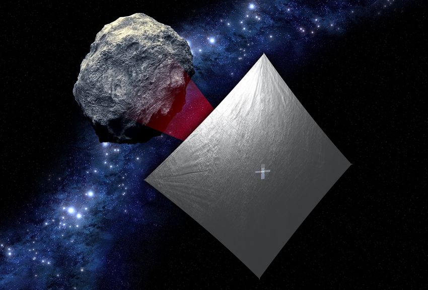
craft can be seen in Figure 1(a). The 86 m2 solar sail is constructed from aluminized colorless polymer
(CP-1) and is shown in Figure 1(b).3, 4 Four flexible, 6.8 m long booms are responsible for deploying the sail
from the initial stowed position in the central 2U of the spacecraft bus.4 Both the sail and the deployment
mechanisim are designed by MSFC and based on the technology developed for NASA’s NANOSail-D and the
Planetary Society’s Lightsail-A.1, 4 Additional propulsion for detumbling and course correction capabilities
is delivered by a cold gas thruster system capable of 38 m/s of total ∆V.5 Attitude control is maintained via
a combination of reaction wheels, active mass translator (AMT), and cold gas thrusters. The four reaction
wheels, each providing 0.004 N-m of torque, are arranged in a pyrimidal formation for redundancy, and
perform the majority of roll, pitch, and yaw maneuvers.6 The active mass translator adjusts the spacecraft’s
∗ Student, Aerospace Engineering and Mechanics, 401 7th Avenue Tuscaloosa, AL 35487, jbpezent@crimson.ua.edu
† Assistant Professor, Aerospace Engineering and Mechanics, 401 7th Avenue Tuscaloosa, AL 35487, rsood@eng.ua.edu
‡ Senior Aerospace Engineer, EV42/Guidance Navigation and Mission Analysis, NASA Marshall Space Flight Center,
Huntsville, AL 35812
1 of 20
American Institute of Aeronautics and Astronautics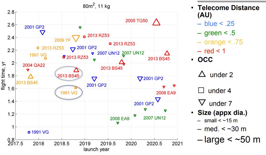
center of mass to center of pressure offset, aiding in maneuvering and momentum desaturation about the
pitch and yaw axis. A ∆V of 5 m/s is also held in reserve to offload the excess momentum accumulated in
NEA Scout’s roll axis.5 The combined system is capable of angular rates of 0.04 deg/s about the pitch and
yaw axis and 0.02 deg/s about the roll axis. NEA Scout’s primary scientific instrument is an ECAM M-50
narrow field-of-view camera provided by JPL. It is capable of high resolution imaging of the target NEA’s
surface. The camera, along with an on-board star tracker, will be used to optically navigate the spacecraft
throughout the planned trajectory.

         (a) The NEA Scout 6U CubeSat bus.6
                                                         (b) An artist’s rendition of NEA Scout surveying a target
                                                         asteroid (1991 VG).1

                                    Figure 1: The NEA Scout spacecraft.

Mission Plan
The current mission plan calls for NEA Scout to be launched as a secondary payload on SLS’s inaugural
flight, Exploration Mission One (EM-1), which will deliver NASA’s Orion capsule on its maiden voyage to the
Moon. Following EM-1’s translunar injection burn and the Orion spacecraft’s separation, NEA Scout will be
ejected from the upper stage of the SLS. The cold gas thrusters will then expend 10 m/s of ∆V to detumble
the rapidly spinning spacecraft and target a planned lunar flyby.7 It will then spend roughly two weeks in
the vicinity of the Moon awaiting for the precise opportunity to depart towards the target asteroid. The
intervening time will be used to deploy the sail and calibrate communications equipment. At the conclusion
of this phase, the cold gas thrusters will perform another small propulsive maneuver, placing the spacecraft
on a trajectory towards its primary target. Thereafter, the spacecraft will be propelled primarily by solar
sail, with 28 m/s of ∆V being held in reserve for any desirable corrective maneuvers. Upon arrival in the
vicinity of the target, NEA Scout will perform a flyby at a velocity of less than 100 m/s relative to the
asteroid from a distance of less than 2 km, and use its on-board camera to characterize the asteroid’s shape,
spectral type, and rotational properties.1, 2, 5 However, there is a considerable interest in how the failure of
the initial outbound trim maneuver and the subsequent lunar flyby will affect the mission’s success.

                                             II.    Objectives
    The goal of this investigation is to explore NEA Scout trajectory options in the event of initial trim
maneuver failure following separation from EM-1. The time-critical nature of the maneuver and limited
available ∆V budget would result in the spacecraft being unable to perform a series of lunar flybys stipu-
lated by the nominal mission plan, and therefore, render the spacecraft incapable of precisely targeting the
necessary departure trajectory. In the intervening time, NEA Scout will fly past the Moon and continue on
an uncontrolled Earth-escape trajectory. The first major corrective actions can only be performed once the
sail and communications equipment have been correctly deployed and calibrated. Thus, this study aims to
design alternative trajectories that start at the J2000 state vector corresponding to the first opportunity for
initial corrective action (ICA-state), and still fulfill NEA Scout’s mission goals.

                                                      2 of 20

                                American Institute of Aeronautics and Astronautics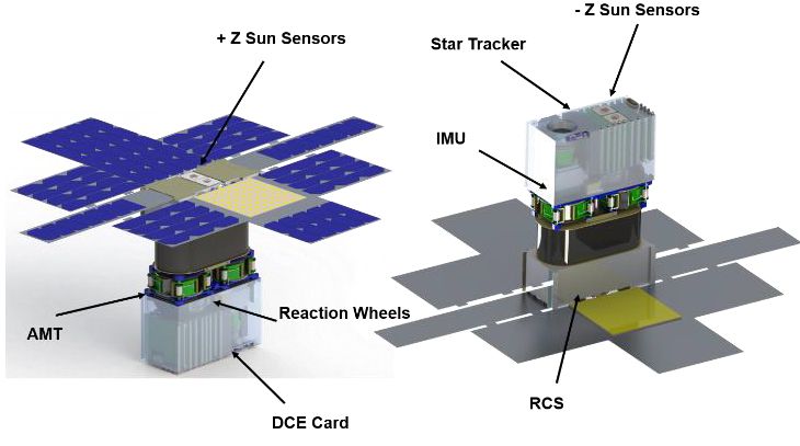
To achieve mission success, the contingency trajectories will need to satisfy the following criteria:
  1. Perform a flyby of the target NEA from a distance of less than 2 km.
  2. At the time of the flyby, the relative velocity should be less than 100 m/s.
  3. The solar sail remains pointed within ± 50◦ of the Sun-sail line.
  4. The spacecraft remains within 1 AU of the Earth.
    Items 1 and 2 represent the low-speed flyby requirement and allow for thorough characterization of the
target asteroid upon arrival. The pointing angle restriction will prevent damage to the spacecraft’s mission-
critical star tracker. The final requirement is a result of NEA Scout’s limited communications range with
Earth-based ground stations.
    The high priority contingency scenario will first be analyzed for the now defunct October 7, 2018 launch
date. The ICA-state was supplied by Marshall Space Flight Center and occurs 17 days after separation
from EM-1 on October 24, 2018. The location of NEA Scout relative to the Earth and Moon in the Sun-
Earth rotating frame can be seen below in Figure 2. Emphasis will be placed on computing and optimizing
trajectories towards this launch date’s primary target, asteroid 1991 VG.

        Figure 2: Sun-Earth rotating frame view of NEA Scout’s ICA-state propagated for 50 days.

    Low-speed flyby trajectories to alternate targets will then be computed and compared to the baseline con-
tingency trajectory to 1991 VG. In addition, a search and assessment of possible high speed flyby trajectories
to both 1991 VG and alternate targets will also be performed.
    During the course of this study, EM-1 was delayed from October 7, 2018 to December of 2019, motivating
a renewed assessment of contingency options. Information from the October 24, 2018 ICA-state will first
be generalized to allow for preliminary analysis of an arbitrary EM-1 launch date. These assumptions will
be used to construct new ICA-states for EM-1 launches in December of 2019. Based on the characteristics
of the resulting initial states, a set of possible rendezvous targets will be selected. Contingency trajectories
to the set of candidate asteroids will then be computed and analyzed in a similar manner to the October 7,
2018 launch date.

                                       III.     Dynamical Model
    To accurately predict the behavior of NEA Scout under multiple gravitational and non-gravitational
forces, a high fidelity dynamical model is developed. The system model is formulated in the international
celestial reference frame (ICRF) and employs ephemeris data for the inertial time-dependent position history
for all bodies under mutual gravitational influence. In addition, an ephemeris formulation for position-
dependent solar radiation pressure is incorporated to model solar sail thrust.

                                                      3 of 20

                                American Institute of Aeronautics and Astronautics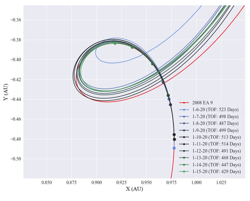
A.    n-body Gravity Model
While Kelplerian and 3 -body gravity models offer excellent tools for preliminary analysis, a higher fidelity
model is necessary to formulate a mission-operable trajectory. To this end, an n-body gravitational model
leveraging NAAIF’s C-Spice system and JPL’s DE 431 planetary and lunar ephemeris is employed. The
gravitational attractions of all relevant celestial bodies acting on the spacecraft may be succinctly stated by
Equation 1.
                                           n
                                          X      µi
                             ~r¨gravity =            2 r̂ic  where      ~ric = ~ri − ~rc                    (1)
                                          i=1 | ~
                                                ric |
Where n represents the number of gravitationally attractive bodies under consideration, µi is the gravi-
tational parameter of the ith body, and ~ric represents the position vector directed towards the ith body
originating at the spacecraft. Since NEA Scout will spend its entire relevant mission profile outside the
sphere of influence of any planetary bodies under the contingency scenario, oblate gravitational effects are
ignored and bodies are assumed to be point masses. The time-dependent position vectors of each body
relative to the solar system’s barycenter ~ri are supplied by JPL’s DE 431 ephemeris.

B.   Solar Radiation Pressure Model
Accurate modeling of the effects of solar radiation pressure (SRP) on NEA Scout’s sail is critical to the
construction of feasible trajectories. Without resorting to finite element analysis, an optical reflection model
offers an excellent approximation of the solar sail’s thrusting capability. The derivation of the model begins
with that of a perfectly flat and reflecting surface of arbitrary shape at a distance of 1 AU from the Sun. In
this form, all incident photons originating from the Sun are assumed to undergo perfectly elastic collisions
with the sail’s surface. Under these assumptions, the acceleration of the sail can be stated in Equation 2.
                                                        2P0 ∗ Asail
                                         ~asail−1AU =               cos2 α n̂                                        (2)
                                                          msail
Where P0 is the SRP at a distance of 1 AU, Asail and msail are the area and mass of the sail-craft, n̂ is the
orientation of the sail in the inertial frame, α is the angle between the sail normal vector and Sun-sail line,
and coefficient 2 arises from the perfect reflection assumption. Direction vector n̂ itself is a function of cone
angle α, clock angle γ, and the position of the sail craft relative to the Sun. A new term βideal can now be
introduced in Equation 3 as the ratio of the local acceleration due to the SRP, and the solar gravity at 1
AU.
                                                                     2
                                                     2P0 Asail | AU |
                                           βideal =                                                           (3)
                                                        msail µsun
βideal , known as the lightness parameter, is the main performance metric of the sail and is constant with
distance from the Sun, owing to the fact that both the SRP and the solar gravity are inverse square fields.8, 9
SRP acceleration at an arbitrary position can now be stated below. As in Equation 1, the Sun’s position ~rs
is determined using the DE 431 ephemeris.
                                                  1        µsun
                                         ~r¨sail = βideal                  2
                                                                   2 (2 cos α n̂)                                    (4)
                                                  2       | ~rsc |

For NEA Scout, with a mass and sail area of 12 kg and 86 m2 , respectively, the ideal lightness parameter
is 0.011. This model can then be modified to account for a non-ideal flat square sail in Equation 5 by
considering the optical properties of the sail’s material.3, 10

            1        µsun                                                                ef Bf − eb Bb
   ~r¨sail = βideal          2   (1 + r
                                      e s) cos2
                                                (α) + B f (1 − s) r
                                                                  e cos (α) − (1 − r
                                                                                   e )                   cos (α)   n̂ (5)
            2       | ~rsc |                                                                ef + eb

                                                  + (1 − res) cos α sin α t̂

                                                         4 of 20

                                   American Institute of Aeronautics and Astronautics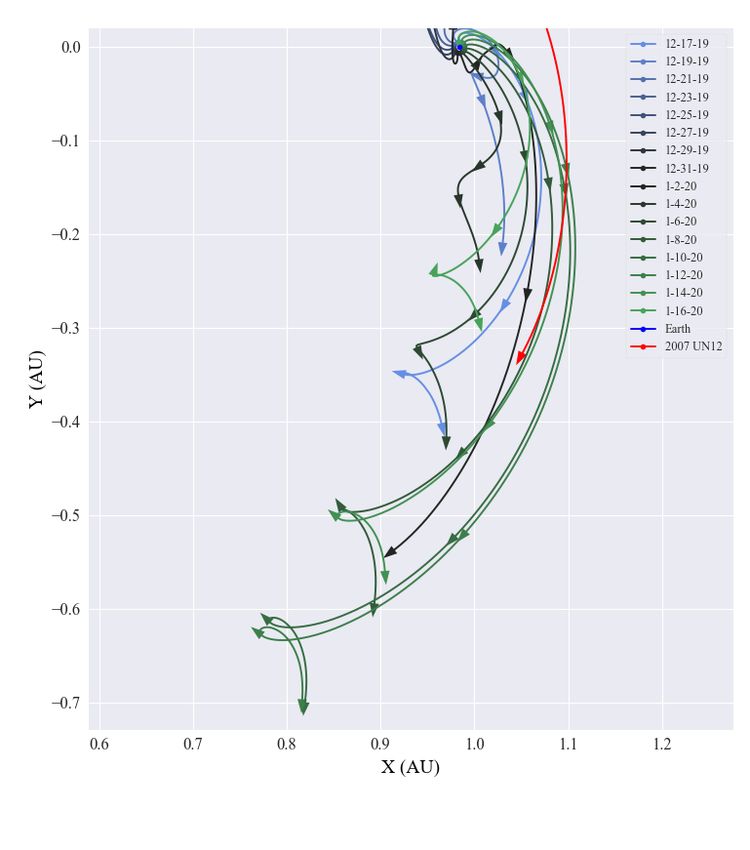
Terms re and s are the reflectivity and specular coefficients. Bf , Bb are the front and backside Lamber-
tian coefficents of the sail, while ef , eb are the front and backside emissivity coefficients. These are based on
updated testing done for the NEA Scout project in 2015 and are available in Table 1.3

                                   Table 1: NEA Scout Optical Coefficients

                                       re       s    Bf     Bb       ef      eb
                                    0.91     0.89   0.79   0.67   0.025    0.27

    The assumption of non-elastic photon collision also introduces a tangential component of SRP accelera-
tion directed in the t̂ direction that is not present in the ideal formulation. Its propulsive effects are small
compared to that of the normal acceleration, but cannot be ignored if one is considering the effects of SRP
torque upon the spacecraft. Such analysis is beyond the scope of this paper, but the propulsive effects are
included and the sail is operated in an α envelope that will mitigate negative impact. The α and γ angles are
not explicitly controlled via modeling of NEA Scout’s attitude control systems. They are, instead, directly
chosen in order to produce the desired orientation.

                                            IV.     Design Strategy
A.     Target and Launch Date Analysis
When designing a contingency trajectory, it is important to first assess the viability of the primary target
asteroid, as well as alternate targets that could potentially present better options. A survey of possible
targets for NEA Scout based on the launch date of EM-1 can be seen in Figure 3 below.
    The given time of flights (TOF)
are based on the assumption that
NEA Scout is able to correctly
perform the planned initial trim
maneuver, and adequately target
the necessary departure trajectory.
Trajectories for a subset of asteroids
chosen for further investigation may
be seen in Figure 4. A 1 AU arc has
been defined relative to the Earth
indicating the communications bar-
rier for the NEA Scout spacecraft.
Each trajectory is shown from Oc-
tober 24, 2018 until the target’s first
crossing of this line.
    Once the initial state when cor-
rective maneuvers can be performed
is defined (ICA-state), trajectory         Figure 3: Possible Target NEAs for variable launch dates.7
options can be directly explored.
However, if the ICA-state is unknown or is subject to change, it is necessary to approximate the state
in a manner that preserves the underlying contingency scenario. The following assumptions are made to
modify an existing ICA-state to an arbitrary launch date.
     1. EM-1’s initial departure trajectory towards the Moon will be similar regardless of the launch date when
        viewed in the Earth-Moon rotating frame.
     2. NEA Scout’s separation and initial lunar flyby targeting maneuver will occur at roughly the same time
        relative to the launch date.
     3. The new ICA-state will still occur the same number of days after separation from EM-1.

                                                       5 of 20

                                 American Institute of Aeronautics and Astronautics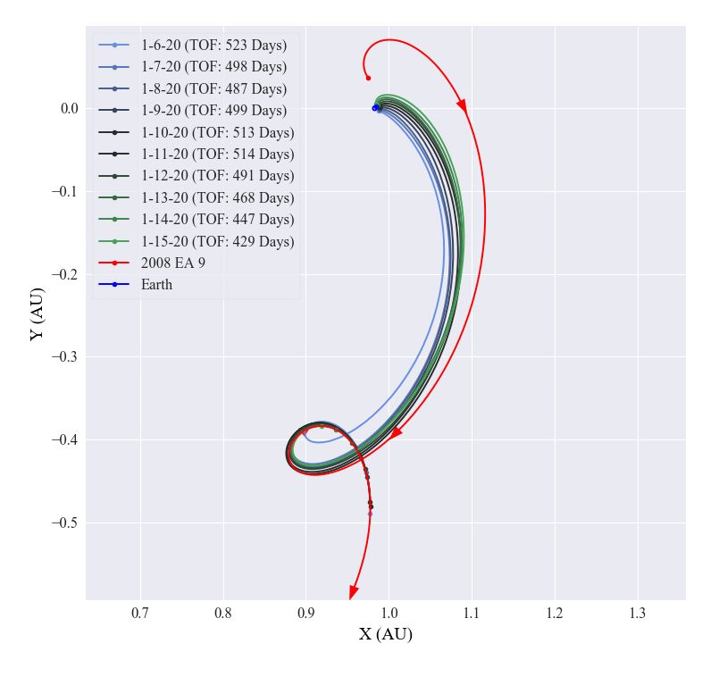
Based on these assumptions, the inertial ICA-state is first transformed into the Earth-Moon rotating frame.
A new EM-1 launch date is chosen, and an additional 17 days are added to account for the time until the
initial corrective action may be performed. The rotating frame ICA-state is then transformed back into the
inertial frame relative to the Earth’s position at the new epoch time. The approximated ICA-state may now
be employed to perform preliminary analysis at the newly specified time.
    For a given ICA-state (true or approximate), a simple heuristic approach is used to assess the feasi-
bility of possible targets. First, a maximum allowable transfer time, Tmax , is calculated from the elapsed
time between NEA Scout’s ICA-state and the target’s first crossing of the 1 AU communications barrier.
A conservative estimate of the minimum possible
transfer time, Tmin , is obtained by considering that
a relative inclination difference, θi , of roughly 0.2◦
at flyby will result in a relative velocity greater than
the 100 m/s requirement. Therefore, Tmin is the
time necessary for NEA Scout to match the orbital
plane of the target. This is calculated by consid-
ering the analytic expression for the maximum rate
of inclination change of an ideal solar sail shown in
Equation 6.
              ∆i = 88.2 βideal deg/orbit              (6)
If it is assumed that NEA Scout has a βideal of .011
and remains at an average 1 AU distance from the
Sun, it can be shown that ∆iavg = .00265 deg/day.
Tmin may then be attained by dividing the relative
inclination between NEA Scout’s initial transfer or-
bit and the target asteroid by ∆iavg as shown in
Equation 8.11, 12
                                                      !
                1                  ~hN EA • ~hT arg
   Tmin = θi        ; θi = acos
              ∆iavg             | ~hN EA || ~hT arg |
                                                       (7)
Terms ~hN EA and ~hT arg represent the specific angu-
lar momentum vectors of the spacecraft and target              Figure 4: Target NEA orbits from October 24,
about the Sun in the ephemeris system. The prox-               2017 until their first crossing of the 1 AU com-
imity of these two times provides a quick indicator of         munications barrier. (Sun-Earth rotating frame)
NEA Scout’s ability to successfully reach the target
asteroid. If Tmin exceeds Tmax , it is fair to assume:

   1. The relative velocity of a flyby occurring at any time before the target’s crossing of the communications
      barrier will be too high to satisfy mission requirements.
   2. High-speed flyby opportunities will be less numerous and restricted to a tighter window around the
      initial orbital nodes of the spacecraft with respect to the target asteroid’s orbital plane.
The same assumptions can be made, but with less certainty, if Tmax is only slightly greater than Tmin .
What constitutes a prohibitively small difference between Tmax and Tmin must be evaluated on a case by
case basis, but can be qualitatively assessed. If it appears that extensive phasing will be required to reach
the target, then a tight Tmax and Tmin bound is likely to result in an inability to match both the phase
angle the inclination before crossing the communications barrier. The above heuristic formulation is by no
means exact, but does give one a good idea of when a contingency trajectory option may be available.

                                                         6 of 20

                                   American Institute of Aeronautics and Astronautics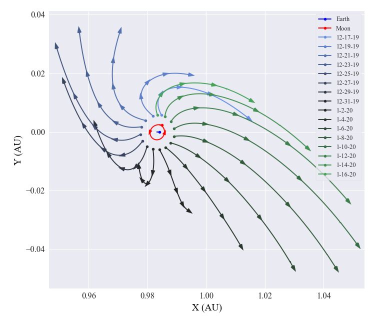
Initial Launch Date Analysis: October 7, 2018
Asteroid 1991 VG was initially selected as the primary target for the October 2018 launch of EM-1, and
under ideal circumstances, represents the most optimal target for a mission beginning in the latter half of
that year.2 Uncontrolled propagation of NEA Scout’s true ICA-state for the 2018 mission, shown in Figure 5,
results in a low inclination trajectory flowing along the Sun-Earth invariant manifolds towards 1991 VG.8, 9
The favourable departure direction bodes well for the possibility of reestablishing a constraint-satisfying tra-
jectory for this launch date. Previous analysis, has indicated that the minimum time of flight for a rendezvous
with 1991 VG is between 600 and 800 days for a nominal 2018 mission scenario.7 This circumvents the pre-
viously described estimate of Tmin , and roughly bounds possible solutions to between 800 and 990 days TOF.

    A quick glance at Figure 3 might suggest that 2013 BS45 is the Table 2: Transfer time bounds for Oc-
next logical option, but the combination of its clockwise heading tober 7, 2018 mission
and location ahead of Earth in the Sun-Earth rotating frame would
likely make it a difficult target for NEA Scout to reach with the
given initial state. The next target listed, 2013 RZ53, appears to      Target  Tmin (days) Tmax (days)
be a viable alternative. It possesses similar location and orbital 1991 VG          452           995
characteristics to 1991 VG when viewed in the Sun-Earth rotating
frame, albeit with a higher inclination relative to the departure 2013 BS45         278          1683
trajectory. Asteroids 2007 UN12 and 2008 EA9 also represent fea- 2013 RZ53          722          1286
sible targets. As seen in Table 2, both asteroids have large upper
bounds on the TOF, but the time needed to correct for the consid- 2007 UN12         334          1619
erable initial phase angle differences could potentially push possible
                                                                       2008 EA9     357          1657
rendezvous towards the high end of the feasibility range.

           Figure 5: 500 day propagation of NEA-Scout’s ICA-state for the October 7, 2018 launch
           date along with potential target asteroids.

                                                      7 of 20

                                American Institute of Aeronautics and Astronautics
New Launch Date Analysis: December 2019
The aforementioned delay of EM-1 to December of 2019 necessitates new ICA-states. A range of possible
initial conditions were computed using the ICA-state from the October 2018 mission. The epoch times,
therefore, can range from December 17, 2019 to January 17, 2020. Uncontrolled 75 day propagation of a
subset of these initial conditions can be seen in Figure 6(a) on the next page.
    Lower bounds on transfer times, Tmin , to each target vary non-linearly with the chosen launch date. The
values given in Table 3 are an average over the previously mentioned time intervals. The 31 day launch
window coupled with 28 day lunar cycle offer considerable control over the general direction of the departure
trajectory. Based on preliminary analysis, 2007 UN12 and 2008 EA9 appear to be favorable targets for
ICA-states ranging from Jan 4, 2020 to Jan 16, 2020. Figure 6(b) and 6(d) highlight the location of 2007
UN12 and 2008 EA9 relative to the favorable ICA-states. On these dates, NEA Scout departs along the
Sun-Earth manifolds heading towards the Sun-Earth L5 Lagrange point while 2008 EA9 and 2007 UN12
follow close behind. Also promising is the small plane change time (Tmin ) for NEA Scout relative to each
target over the entirety of the launch month. Additionally, Tmax for each target is on average 1200 days,
providing considerable time for maneuvering. With the addition of sail control, the spacecraft can potentially
rendezvous with these targets sooner than the equivalent 2018 mission.
    For the remainder of the launch window, asteroid 2013 BS45 appears to be a good choice for a rendezvous
target. This asteroid possesses a larger initial phase angle with respect to NEA Scout than 2007 UN12 or 2008
EA9, but retains a high upper bound on flight time. As seen in Figure 6(c), the trajectories flow towards
the Sun-Earth L4 Lagrange point and close the existing phase angle within 800 to 900 days. Extensive
maneuvering will be required to arrive at low speeds relative to the target asteroid, but the relatively small
Tmin will allow for NEA Scout to spend the majority of the trajectory thrusting in plane with 2013 BS45.
    Asteroids 1991 VG and 2013 RZ53, however, seem to be poor targets compared to the previous launch
date. In both cases, the additional 420 days has brought the Tmin - Tmax bounds close together, and violated
the bounds in the case of 2013 RZ53. This implies that the time spent changing inclination will dominate
the sail maneuvering schedule, leaving little time to overcome the now larger phase angles.

                   Table 3: Average transfer time bounds for a December 2019 mission.

                                     Target       Tmin (days)     Tmax (days)
                                   1991 VG            380              575
                                  2013 BS45            95             1263
                                  2013 RZ53           945              866
                                  2007 UN12           340             1199
                                   2008 EA9           120             1237

                                                      8 of 20

                                American Institute of Aeronautics and Astronautics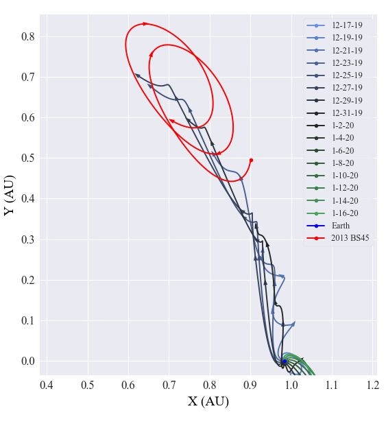
(a) ICA-state propagation for 75 days - Moon in red.

                                                          (b) ICA-state propagation for 500 days - 2008 EA9 in red.

  (c) ICA-state propagation for 800 days - 2013 BS45
  in red.
                                                       (d) ICA-state propagation for 500 days - 2007 UN12 in red.

Figure 6: Propagation of updated ICA-state vectors as viewed in the Sun-Earth rotating frame. The legend
indicates the date of each initial state. The motions of the Earth and Moon are shown only from December
17, 2019 to January 16, 2020. Note: The near circular lunar orbit and initial state spacing are due to Earth
reaching perihelion on January 4, 2020 in the middle of the displayed time range.

                                                       9 of 20

                                American Institute of Aeronautics and Astronautics
B. State-Space Model
Prior to investigating trajectories to one of the proposed targets, a discrete state-space model for the trajec-
~ L,
tory and relevant mission constraints is constructed. This is done by first defining the entire trajectory, X
~
as a vector of n discrete states, Xi .
~rc
X~1
~ ~r˙
X c
X~ L = .2 ; ~i =
X t (9 × 1)
(8)
.
.
α
X~n γ
Vectors ~rc and ~r˙c represent the x-y-z components of the spacecraft’s position and velocity relative to the
solar system’s barycenter. Element t is the epoch time of the state and determines the true positions of all
bodies in the ephemeris formulation for n-body gravitation and SRP. As stated earlier, cone angle, α, and
clock angle, γ, orient the normal vector and thrust of the sail relative to the Sun-sail line and by geometrical
transformation to the solar system’s barycenter. From Equations 1 and 2, a discrete model can be expressed
for the time derivative of the spacecraft’s state, X ~˙ i . Equation 9 assumes that α and γ are discrete control
variables, and that time is linearly represented.
→−̇
r c (3 × 1)
→−̈
r c (3 × 1)
˙~
Xi = 1 (9 × 1) W here ~r¨c = ~r¨sail + ~r¨gravity (9)
0
0
Construction of a total mission constraint vector begins by first considering the boundary conditions for a
successful contingency trajectory. The initial state constraint, denoted C~ s (X
~ 1 ), enforces that the trajectory
begins at pre-specified ICA-state dictated by the chosen launch date. Terms Cp (X ~ n , bp ) and Cv (X
~ n , , bv )
n n
represent the terminal conditions of a low speed flyby with the target asteroid.
~ s (X
C ~ 1) = X
~1 − X
~ ICA = ~0 [1 : 7] (10)
~ n , bp ) = 2.0 km − |~rc − ~rT arg [tn ]| − |bp | = 0
Cp (X (11)
n n
~ n , bvn ) = 100 m/s − |~r˙c − ~r˙T arg [tn ]| − |bvn | = 0
C v (X (12)
The non-negative terms, bvnand bpn ,
known as slack variables, convert the original inequality constraints into
equality constraints. Additional constraints must now be placed upon the cone angle, α, in each state. For
each X~ i this constraint can also be expressed with the aid of additional slack variables.
" #
u
~ α (X
~ i) = 50 − α − |b |
C i = ~0 (13)
α − |bli |
~ and all constraints are appended to vector, C(
All slack variables are stored in the slack vector, B, ~ X~ L , B).
~
u
b1
bl
1 C~ s (X1 )
u
b2
Cp (X ~ n , bp )
n
~ n , bvn )
l
b2 Cv (X
B = ...
~ ; ~ ~ ~
C(XL , B) = ~ α (X1 , bl , bu )
C (14)
1 1
bu
~ α (X2 , bl , bu )
C
n
2 2
l
..
bn .
~ α (X
~ n , , bln , bun )
bpn C
bvn
10 of 20
American Institute of Aeronautics and Astronautics~ L and slacks in B
In this form, the converged solution will satisfy the constraints if the states in X ~ satisfy
~ X
C( ~ L , B)
~ = ~0.
C. Control Law Initial Guess Construction
To initialize the trajectory vector X ~ L , a simplified locally-optimal control law is used to construct a partial
transfer onto the target’s orbit from the initial state X ~ 1 . The control law, similar to that described by
Petropolus and Dachwald, is formulated by converting the instantaneous state of both the sail craft, X ~ i , and
~
the target asteroid, XT arg , into sets of five classical orbital elements describing their osculating orbits about
the Sun.12–14 A function ‘Q’ may then be constructed which quantifies the ‘distance’ between the orbit of
the sail and the target. Q is the sum of the differences between each orbital element divided by the maximal
rate of change possible over the current set of orbital elements.13
ai − aT arg
!2 e −e
5 ~ i T arg
X ∆O[j] ~ =O
~i − O
~ T arg
Q= = where ∆O = ii − iT arg (15)
˙~
j=1 ∆Omax [j]
Ωi − ΩT arg
ωi − ωT arg
The control law chooses an α and γ to orient the solar sail in a direction that will instantaneously minimize
Q̇, the time rate of change of Q.11 NEA Scout is then propagated under this set of sail controls in the full
force model for a finite amount of time, after which the process is repeated. At each minimization of Q, the
current state X~ i is concatenated into the vector X
~ L in order to construct the initial state and control history
for the spacecraft. Under ideal circumstances the control law will eventually yield a trajectory which arrives
on or close to the target’s osculating orbit, but not necessarily at the target object. In fact, the lack of
control over the spacecraft’s initial true anomaly can lead to the target and spacecraft having a large phase
angle difference at the solution of Q.12, 13 For this reason, the control law is typically not run until Q = 0.
Instead, it is terminated once the spacecraft makes a sufficiently close approach with the target. Despite
these limitations, the law supplies a viable initial guess for the sail control history.
D. Trajectory Transcription
Given an initial guess for X~ L , 7th order Gauss Lobatto collocation is used to transcribe the equations of
motion into a form suitable for efficient numerical solving and optimization. This technique is an example of
the popular direct transcription class, and was first described by Hermann and Conway.15, 16 Analysis has
shown the method to be more effective than other direct transcriptions in trajectory optimization problems.17
The method constructs 7th order polynomials between states X ~ i in the total design vector X
~ L . The equations
of motion are considered satisfied if the resulting time-derivative of this piecewise polynomial matches that
of the underlying system dynamics at predefined ‘collocation’ points.18 These polynomials along with the
~ X~L ,B)
mission constraints, C( ~ can be solved for simultaneously to yield a feasible trajectory.
th
For a single 7 order Lobatto polynomial arc, 4 successive ‘node’ states X ~ N through X ~ N in X
~ L are
1 4
17, 19–21 th
necessary (superscript N is applied for clarity). The unique 7 order polynomial is then constructed
and evaluated at the three interior collocation points. This entire process can be summarized in a common
Equation 16 for the ith collocation point.
~ iC [1 : 6] = (ai1 X
X ~ 1N + ai2 X
~ 2N + ai3 X
~ 3N + ai4 X ~˙ 1N + bi2 X
~ 4N + ∆t(bi1 X ~˙ 2N + bi3 X
~˙ 3N + bi4 X
~˙ 4N ))[1 : 6] (16)
~ iC [7] = X
X ~ 1N [7] + τi ∆t
~ iC [8 : 9] = X~N [8 : 9]
X i
Sail angles α and γ at the ith collocation point are assumed to be piecewise constant and inherited from
the ith node state. In this formulation, the total arc time is free to move by varying the epoch times at
the first and last node states. The ‘defect’ equation, δ~i , representing the difference between the polynomial
11 of 20
American Institute of Aeronautics and Astronauticsderivatives and the true derivatives at each of the three collocation points then takes the common form of
Equation 17.
i ~˙ N i ~˙ N i ~˙ N i ~˙ N i ~˙ C
δ~i = (ei1 X
~ N + ei X
1
~N i ~N i ~N ~
2 2 + e3 X3 + e4 X4 + ∆t(f1 X1 + f2 X2 + f3 X3 + f4 X4 + f5 Xi ))[1 : 6] = 0 (17)
The full constraint equation to be satisfied for a single Gauss Lobatto arc can be seen in Equation 18.
~δ1
F~ (X
~1 , X
N ~2 , X
N ~3 , X
N ~ 4 ) = ~δ2
N
= ~0 (18)
~δ3
Additional constraints, which have been omitted for brevity, are employed to strictly enforce both the forward
direction of time, and the correct time spacing of the two interior node states on the normalized time interval
between X ~ N and X~ N . The node state spacings, along with the coefficients shown above, are unique to 7th
1 4
order Gauss Lobatto collocation, and their precise values can be found in the referenced works of Grebow
and Ozimek.20, 21
An entire piecewise representation of the trajectory is created by linking each Lobatto arc together at the
first and last node state. The defect equations for each arc can be added, along with the mission constraints,
into a single vector F~ (X
~ L , B)
~ shown in Equation 19.
F~ (X
~ 1, X
~ 2, X
~ 3, X
~ 4)
F~ (X
~ 4, X
~ 5, X
~ 6, X
~ 7)
~ ~ ~
F (XL , B) =
.
..
(19)
F~ (X
~ 3m−2 , X
~ 3m−1 , X ~ 3m , X
~ 3m+1 )
~ ~
C(XL , B) ~
For a trajectory consisting of m Lobatto arcs, the number of states, n, must obey n = (3m+1). As an
additional error check, collocation solutions are also verified with a multiple shooting algorithm. Each X ~ i is
explicitly integrated to the epoch time of X ~ i+1 in the trajectory vector, X ~ L . To satisfy the system dynamics,
the trajectory must be continuous in both position and velocity between states. This can be expressed via
Equation 20 where X ~ i (ti+1 ) represents the integration of the ith state to the epoch time of X ~ i+1 . Equation
~
20 then replaces the defect equations in F (XL , B). ~ ~
F~ (X~ 1, X
~ 2)
~ ~ ~
F (X2 , X3 )
F~ (X
~ i, X
~ i+1 ) = (X~ i (ti+1 ) − X~ i+1 )[1 : 6] ; F~ (X
~ L , B)
~ =
..
(20)
.
~ ~ ~
F (Xn−1 , Xn )
~ X
C( ~ L , B)
~
The independence of each arc helps to distribute any error remaining in a solution throughout the entire
trajectory. Similar to collocation, TOF is allowed to vary by choosing the epoch time of the individual states.
Likewise, sail angles α and γ are assumed piecewise constant along the ith arc and inherited from X ~ i .8 The
multiple shooting scheme is accurate to the tolerances of the underlying integration method, therefore its
convergence assures the accuracy of the solution.
E. Trajectory Targeting
In aerospace trajectory design, directly solving F~ (X ~ L , B)
~ is often referred to as targeting. In this case,
regardless of whether collocation or multiple shooting is used, the targeting problem is a large non-linear
system of equations consisting of several thousand constraints and independent variables. This must be
solved via an iterative Newton-type method. Given an initial guess for X ~ L i , Newton’s method takes the
form of Equation 21.9, 20–22
" # " #
~ L i+1
X X~L i −1
= − DF~ (X
~ L i, B
~ i )T DF~ (X ~ L i, B
~ i ) DF~ (X
~ L i, B
~ i )T F~ (X
~ L i, B
~ i) (21)
~ i+1
B ~i
B
12 of 20
American Institute of Aeronautics and AstronauticsTerm DF~ (X ~ L , B)
~ is the Jacobian matrix consisting of the partial derivatives of F~ (X ~ L , B)
~ with respect
~ ~
to each variable in XL and B. The Jacobian computed at each iteration typically contains over 1 million
elements. Fortunately, the discretization of the trajectory into independent Lobbatto or shooting arcs results
in a sparse problem where at least 99 percent of Jacobian entries are equal to zero. These can be ignored
when computing DF~ (X ~ L , B).
~ High performance linear-algebra libraries are used to solve the sparse linear
19
system in Equation 21.
In most cases, the initial X ~ L provided by the control law is sufficient to allow for solution to F~ (X ~ L , B).
~
~
If not, the algorithm may not converge, necessitating either another guess for XL from the control law, or
attempting to solve a ‘relaxed’ version of F~ (X ~ L , B).
~ One common relaxation employed in this situation is
raising the maximum flyby velocity restriction appended to the end of F~ (X ~ L , B)
~ until a solution can be
found.
~ n , bvn ) = (100 + Vrelax ) m/s − |~r˙n − ~r˙T arg (tn )| − |bvn | = 0
C v (X (22)
The scalar Vrelax is the amount by which the flyby velocity restriction will be increased. The solution to
this relaxed problem can then be used as a new guess to the original problem.
F. Trajectory Optimization
Once a set of feasible solutions has been found, it is critical to search for optimal trajectories that minimize
total mission cost compared to the baseline. Since a solar sail spacecraft expends no fuel for propulsion, one
of the most relevant cost metrics to minimize in pursuit of this goal is the total time of flight (TOF). This
optimization problem is formally stated below.
n−1
X
M inimize : ~ L) =
T (X ~ i+1 [7] − X
(X ~ i [7])2 (23)
i=1
F~ (X
~ 1, X
~ 2, X
~ 3, X
~ 4)
F~ (X
~ 4, X
~ 5, X
~ 6, X
~ 7)
Subject to : F~ (X
~ L , B)
~ =
.. = ~0
.
F~ (X
~ n−3 , X
~ n−2 , X~ n−1 , X
~ n )
~ X
C( ~ L , B)
~
The cost function T (X ~ L ) is the sum of the differences in the epoch time of each successive state in the
design vector squared. Defining the TOF cost in this manner allows for contribution from every state in
the design vector, and helps restrict non-feasible solutions. Term F~ (X ~ L , B)
~ represents the dynamical and
mission constraints outlined previously. Similar formulations are also used to minimize both flyby distance
and velocity when required.
Local optimization of a cost function is performed via Sequential Quadratic Programming (SQP) which
successively minimizes a quadratic model of the objective function, T (X ~ L ), subject to a linearization of the
~ ~ ~
non-linear constraints F (XL , B). 23, 24
As with targeting, optimization of a trajectory is initially performed
with a collocation transcription and refined with multiple shooting once a solution has been found. By
providing a feasible initial guess for X ~ L , SQP will generally return a lower cost trajectory, however, there
is no guarantee that this solution will be globally optimal. Unfortunately, trajectory optimization problems
have many strong local minimums and saddle points which prevent convergence to the true global optimum.
Attempts to mitigate this issue are made by starting the algorithm from many different initial trajectory
guesses and directly targeting lower cost solutions when perceived local minima are encountered.
V. Results
A. Initial Launch Date Results: October 7 2018
The most pressing issue to be addressed for the October 2018 launch date was the viability of the primary
mission to 1991 VG. Initial propagation using the control law suggested that a low-speed flyby or rendezvous
was possible in the 800 to 990 day feasibility range. One such run for 875 days is depicted in Figure 7. The
Q law was not able to arrive precisely at 1991 VG, but was able to reduce both the phase angle and target
13 of 20
American Institute of Aeronautics and Astronauticsseparation at 875 days as compared to uncontrolled propagation.The initial guesses for the trajectory vector
X~ L were then provided to a collocation targeter configured to find a flyby trajectory (free velocity restriction).
The high convergence radius of the algo-
rithm yielded quick solutions even when
provided with poor initial guesses. At
this stage of the process, flyby speeds of
(200 - 700) m/s were typical at TOFs of
800 to 1100 days. An SQP minimization
algorithm with a terminal flyby velocity
cost function was then used to lower the
flyby speed until the 100 m/s requirement
was met. These solutions were passed
to another SQP algorithm configured to
minimize the TOF along with the slacked
flyby velocity constraint to keep new so-
lutions bounded below the 100 m/s re-
quirement. Once a local minimum for
the TOF was reached, the trajectories
were re-converged and optimized under
the same cost function and constraints
using a refined collocation mesh and mul-
tiple shooting. The process was success-
ful in bringing the flyby speed to 80 m/s
and minimizing the TOF to 873 days. Al-
though the algorithm consistently yielded
Figure 7: Position of NEA Scout and 1991 VG
final solutions at this TOF, it is not guar-
after 875 days of control law propagation.
anteed that that this is the globally opti-
mal solution for the given ICA-state.
As expected, the TOF of a low-
speed flyby of 1991 VG appears to have
increased considerably compared to a
nominal trajectory (873 vs 800 days).
To achieve full rendezvous (0 m/s rel-
ative velocity), an additional 7 days of
transfer time is necessary. Addition-
ally, the collocation and shooting tar-
geting scheme was configured to search
for high speed flybys over a TOF range
of 200 to 1000 days. A sample of con-
verged trajectories and their correspond-
ing flyby speeds can be found in Table 4.
Of particular interest and possible utility
is the solution corresponding to a TOF
of 263 days. It was identified upon find-
ing that nearly all converged trajectories
in 800 to 1100 day TOF range also made
close approaches within 5 million kilome-
ters during this time. This indicated that
double flyby opportunity might be avail-
able. Extensive targeting and local op-
timization were used compute a range of Figure 8: A low-speed flyby with 1991 VG
flybys over this time period. The final viewed in the Sun-Earth rotating frame. The
flyby velocity of 1.43 km/s still greatly red arrows indicate the direction of the sail
exceeds that required for the full mission normal vector, n̂.
success criteria as outlined in section 2,
14 of 20
American Institute of Aeronautics and Astronauticsbut could be sufficient to achieve partial target characterization early in the mission. Mission operators
would have the choice to continue on to a second flyby/rendezvous with 1991 VG, or to divert to another
target NEA. Such a maneuver could be necessary in the (highly) unlikely event that 1991 VG were discovered
to be a spent Saturn 5 upper stage as some have speculated in the past.25 The combination of this flyby
with a return to rendezvous with 1991 VG at T + 970 days is depicted in Figure 9. Note that the spacecraft
is still within the communications range.
Figure 9: A high speed flyby of 1991 VG at T + 263 days to rendezvous at T+ 970 days. Lower
speed early flyby’s of 1.0 km/s are available in the 280 - 300 day TOF range, but can potentially
put the second flyby at jeopardy of occurring too close to the communications barrier.
Once the major questions regarding 1991
VG were addressed, work was directed at eval- Table 4: Sample early flyby trajectories of 1991 VG for the
uating the other feasible targets in the design October 7, 2018 mission.
space outlined in section 4. The most promis-
ing of these candidates was asteroid 2013 RZ53.
The same targeting sequence was applied in or- TOF (days) Flyby Distance (km) Flyby Speed (km/s)
der to converge mission operable trajectories. 263 1.83 1.43
One rendezvous solution with a TOF of 1016
days is depicted in Figure 10(a). The additional 441 0.57 1.06
transfer time of 150 days can be attributed to 611 2.21 0.65
2013 RZ53’s higher inclination relative to NEA
Scout’s initial orbit (Tmin = 722 days), neces- 716 1.33 0.16
sitating large amounts of time thrusting out of
plane. Since 2013 RZ53 was still 250 days away from its Tmax , it was possible to exploit the aforementioned
early flyby of 1991 VG. A two phase trajectory combining the same early flyby of 1991 VG followed by a
rendezvous with 2013 RZ53 at 1200 days can be seen in Figure 10(b). This trajectory could present a good
15 of 20
American Institute of Aeronautics and Astronauticsalternative option should mission operators wish to divert from a rendezvous with 1991 following the initial
encounter. Trajectories to the remaining asteroids that were surveyed (2007 UN12, 2008 EA9) required
considerably longer mission times in order to satisfy all mission constraints. While all of the relevant mission
requirements are met, it would be difficult to justify the additional 300 days TOF as compared to a 1991
VG or 2013 RZ53 trajectory.
Table 5: Additional sample low speed flyby trajectories for the October 7, 2018 Mission
Target TOF (days) Flyby Distance (km) Flyby Speed (m/s)
1991 VG 880 0.6 2.3
2013 RZ53 1056 1.5 15.5
2007 UN12 1353 0.9 63.2
2008 EA9 1316 0.3 74.5
(b) A 1991 VG flyby to 2013 RZ53 rendezvous trajec-
(a) 2013 RZ53 rendezvous trajectory. The sail spends tory. Note that this is the same flyby as previously
the majority of the trajectory pointing 30 ◦ - 36 ◦ mentioned, allowing NEA-Scout to immediately di-
below or above the spacecraft’s orbital plane. Note vert to 2013 RZ53 if it were decided to abort a second
that when viewed in the Sun-Earth rotating frame, encounter with 1991 VG.
2013 RZ53 spends a disproportionately long amount
of time in the ‘crests’ of the displayed orbit.
Figure 10: 2013 RZ53 trajectory options.
16 of 20
American Institute of Aeronautics and AstronauticsB. New Launch Date Results: December 2019
Work thus far has shown asteroid 2008 EA9 to be a desirable target in terms of TOF and communications
distance for the December 2019 mission. A low TOF trajectory to 2008 EA9 is illustrated in Figure 11(a) on
the next page. It assumes an EM-1 launch date of December 22, 2019 and enables NEA Scout to perform a
low-speed flyby (73 m/s) in just 410 days. The short transfer time is due to the small phase angle between
NEA Scout and the target at the outset of the contingency scenario as well as the θi of 0.28 deg. This allows
NEA Scout to spend the majority of the time phasing with the target rather than matching inclinations.
One can note the importance of an optimal departure trajectory by comparing the rendezvous time with
2008 EA9 in 2019 with that in 2018. The TOF, plus the additional time between launch dates, is still less
than that of the equivalent 2018 mission.
The second best asteroid target in terms of TOF and communications distance was identified as 2007
UN12. A rendezvous trajectory with a launch date of December 19, 2019 and TOF of 693 days can be seen
in Figure 11(b) on the next page. This particular solution, has NEA Scout loiter in close proximity of the
Earth while matching target inclinations. The spacecraft then departs for 2007 UN12 once it has crossed
below Earth’s position as viewed in the Sun-Earth rotating frame. While TOF is still considerably smaller
than any option from the October 2018 mission, the 300 day loop implies that the optimal launch date is
likely roughly 300 days in the future. This could make 2007 UN12 an attractive low TOF target should
EM-1 be delayed into 2020.
Asteroid 2013 BS45 was the third best option based off of the aforementioned metrics. A typical ren-
dezvous trajectory with a TOF of 843 days is shown in Figure 11(c) on the next page. The departure
trajectory results in a θi of .06 degrees, meaning that NEA Scout can spend the majority of the trajectory
thrusting in plane to phase with the target. Despite the higher TOF, 2013 BS45 presents a unique option
compared to the previously mentioned targets. The asteroid is flowing away from Earth and towards the
Sun-Earth L4 Lagrange point. In fact, the nominal orbit of 2013 BS45 seems similar to that of an L4
periodic orbit at the time of its crossing of the 1 AU communications barrier.9 The converged trajectory
can be leveraged to insert the spacecraft into an orbit about L4 after a successful flyby of 2013 BS45. An
assessment of the feasibility and utility of this option will be the subject of future investigations.
Table 6: Additional sample of low speed flyby trajectories for December 2019
Target Launch Date TOF (days) Flyby Distance (km) Flyby Speed (m/s)
2013 BS45 12-10-19 815 1.41 86.2
2008 EA9 12-29-19 415 0.15 79.7
2007 UN12 12-21-19 685 0.56 94.4
17 of 20
American Institute of Aeronautics and Astronautics(b) A 693 day TOF rendezvous trajectory with 2007
(a) A 410 day TOF low-speed flyby trajectory (73 UN12. The ICA-state occurs on January 5, 2020
m/s) to 2008 EA9. The ICA-state occurs on January corresponding to a launch date of December 19, 2019.
9, 2020 corresponding to a launch date of December TOF is on average higher than that of 2008 EA9
22, 2019. Trajectories to 2008 EA9 have the shortest due to less favorable departure inclinations and phase
TOF of any target thus far surveyed in this study. angles.
(c) An 843 day TOF rendezvous trajectory with 2013 BS45. The ICA-state occurs on December 27, 2020
corresponding to a launch date of December 10, 2019. Despite being a higher TOF target for the majority
of the month, 2013 BS45 is more accessible than 2008 EA9 and 2007 UN12 for launch dates in the first 2
weeks of December 2019.
Figure 11: Sample trajectories to 2007 UN12, 2008 EA9, and 2013 BS45.
18 of 20
American Institute of Aeronautics and AstronauticsAttempts were also made to compute trajectories to 1991 VG and 2013 RZ53, but so far no constraint
satisfying solutions have been found for the December 2019 launch window in the case of trim maneuver
failure. As expected, the one year launch delay seems to have placed both asteroids too far out of range.
NEA Scout is unable to rendezvous with either target before it crosses the 1 AU communication distance
barrier.
The exact launch date of EM-1 in December of 2019 has not yet been determined, and once defined,
could still be subject to local launch delays. Therefore, it is prudent to establish contingency options for
a range of possible launch dates over the launch window. One such set of solutions for 2008 EA9 can be
seen in Figure 12. As was evident from Figure 6, launch dates between December 20 and 31 resulted in
departure trajectories that seemed favorable to this target. A family of rendezvous trajectories to 2008 EA9
were then computed over this date-range via single parameter continuation in ICA-state epoch time. TOF
varies considerably, but remains within a readily acceptable 430-530 day range. These times are subject to
improvement with further optimization. Similar trajectory families can also be constructed for the launch
dates conducive to missions to 2013 BS45 and 2007 UN12.
(b) A close up of rendezvous locations between
NEA Scout and 2008 EA9.
(a) An overall view of the trajectory family to-
wards asteroid 2008 EA9.
Figure 12: A family of rendezvous trajectories to asteroid 2008 EA9. The single parameter continuation
scheme in the ICA-state epoch time began at 1-6-20 and progressed in 6 hour increments until 1-15-20. The
trajectory solution for the previous ICA-state provided the initial guess for the next. Only 1 trajectory per
calendar day is shown. The sail normal vectors, n̂, have been removed for clarity.
In the future, once a concrete launch date and nominal trajectory have been defined, it will be possible
to re-evaluate trajectory options under the same constrained circumstances as the previous October 7, 2018
mission. If the mission profile remains consistent, the preliminary solutions found above will provide an
excellent starting point for a more thorough analysis.
VI. Conclusion and Future Work
The work presented in this study suggests that even with the failed trim maneuver and lunar flyby, the
NEA Scout mission is still capable of achieving its primary goals. Solar sail trajectories to initial target
asteroid, 1991 VG, and alternative targets were designed, optimized, and assessed based on the initial
conditions from the previously defined launch date of October 7, 2018. Rendezvous with the primary target,
1991 VG, still represented the most optimal mission profile in terms of TOF, however, with the change
in launch date, low-speed flyby is uncertain. Alternatively, trajectories to other NEAs presented feasible
19 of 20
American Institute of Aeronautics and Astronauticssolutions that can potentially replace or augment the baseline contingency trajectory. Initial work was also
performed to update this study for EM-1’s new tentative December 2019 launch date. Asteroids 2013 BS45,
2008 EA9, and 2007 UN12 were identified as promising targets for missions beginning in the second half of
December 2019. Multiple rendezvous trajectories were computed to each target asteroid for varying launch
dates. The investigation presented in this paper shows that the December 2019 launch scenario provides NEA
Scout with numerous alternate NEAs and potential contingency options. Additional work, in collaboration
with Marshall Space Flight Center, will be carried out to verify NEA Scout trajectory solutions for specific
launch dates and the next target asteroid.
Acknowledgments
All work was performed using facilities, equipment, and software provided or created by the University
of Alabama’s Astrodynamics and Space Research Laboratory.
References
1 Johnson, L., McNutt, L., and Castillo-Rogez, J., “Near Earth Asteroid (NEA) Scout Mission,” 2017.
2 McNutt, L., Johnson, L., Clardy, D., Castillo-Rogez, J., Frick, A., and Jones, L., “Near-Earth asteroid scout,” 2014.
3 Heaton, A., Ahmad, N., and Miller, K., “Near Earth Asteroid Scout Solar Sail Thrust and Torque Model,” 2017.
4 Sobey, A. R. and Lockett, T. R., “Design and Development of NEA Scout Solar Sail Deployer Mechanism,” 2016.
5 Heaton, A., private communication, 2017.
6 Orphee, J., Diedrich, B., Stiltner, B., Becker, C., and Heaton, A., “Solar Sail Attitude Control System for the NASA
Near Earth Asteroid Scout Mission,” 2017.
7 Carlisle, G., Landau, D., Grebow, D., Lantoine, G., Nandi, S., Gustafson, E., Riedel, E., Laipert, F., and Stuart, J.,
“Concurrent Mission Design of NEA Scout and Lunar Flashlight, Solar Sail CubeSat Missions,” 2015.
8 Sood, R. and Howell, K., “L4, L5 Solar Sail Transfers and Trajectory Design: Solar Observations and Potential Earth
Trojan Exploration,” .
9 Sood, R., Significance of specific force models in two applications: Solar sails to sun-earth L 4/L 5 and grail data analysis
suggesting lava tubes and buried craters on the moon, Ph.D. thesis, Purdue University, 2016.
10 Wie, B., Space vehicle guidance, control, and astrodynamics, American Institute of Aeronautics and Astronautics, 2015.
11 Abd El-Salam, F., “Some new locally optimal control laws for sailcraft dynamics in heliocentric orbits,” Journal of
Applied Mathematics, Vol. 2013, 2013.
12 Macdonald, M. and McInnes, C. R., “Analytical control laws for planet-centered solar sailing,” Journal of Guidance
Control and Dynamics, Vol. 28, No. 5, 2005, pp. 1038.
13 Petropoulos, A. E., “Simple control laws for low-thrust orbit transfers,” 2003.
14 Dachwald, B., Low-thrust trajectory optimization and interplanetary mission analysis using evolutionary neurocontrol,
Ph.D. thesis, Doctoral thesis, Universität der Bundeswehr München Fakultät für Luft-und Raumfahrttechnik, 2004.
15 Herman, A. L. and Conway, B. A., “Direct optimization using collocation based on high-order Gauss-Lobatto quadrature
rules,” Journal of Guidance Control and Dynamics, Vol. 19, No. 3, 1996, pp. 592–599.
16 Topputo, F. and Zhang, C., “Survey of direct transcription for low-thrust space trajectory optimization with applications,”
Abstract and Applied Analysis, Vol. 2014, Hindawi Publishing Corporation, 2014.
17 Ozimek, M. T., Grebow, D. J., and Howell, K. C., “A collocation approach for computing solar sail lunar pole-sitter
orbits,” Open Aerospace Engineering Journal, Vol. 3, 2010, pp. 65–75.
18 Wawrzyniak, G. and Howell, K. C., “Numerical methods to generate solar sail trajectories,” 2nd International Symposium
on Solar Sailing, New York City College of Technology, City University of New York,(Brooklyn, New York), 2010, pp. 195–200.
19 Grebow, D. J., Ozimek, M. T., and Howell, K. C., “Design of optimal low-thrust lunar pole-sitter missions,” The Journal
of the Astronautical Sciences, Vol. 58, No. 1, 2011, pp. 55–79.
20 Ozimek, M. T., Low-thrust trajectory design and optimization of lunar south pole coverage missions, Ph.D. thesis, Purdue
University, 2010.
21 Grebow, D. J., Trajectory design in the Earth-Moon system and lunar South Pole coverage, Ph.D. thesis, Purdue
University, 2010.
22 Betts, J. T., “Survey of numerical methods for trajectory optimization,” Journal of guidance, control, and dynamics,
Vol. 21, No. 2, 1998, pp. 193–207.
23 Barclay, A., Gill, P. E., and Rosen, J. B., “SQP methods and their application to numerical optimal control,” Report
NA, 1997, pp. 97–3.
24 Gill, P. E., Murray, W., and Saunders, M. A., “SNOPT: An SQP algorithm for large-scale constrained optimization,”
SIAM review , Vol. 47, No. 1, 2005, pp. 99–131.
25 de la Fuente Marcos, C. and de la Fuente Marcos, R., “Dynamical evolution of near-Earth asteroid 1991 VG,” Monthly
Notices of the Royal Astronomical Society, Vol. 473, No. 3, 2017, pp. 2939–2948.
20 of 20
American Institute of Aeronautics and AstronauticsYou can also read