Novel free-form optical surface design with spiral symmetry
←
→
Page content transcription
If your browser does not render page correctly, please read the page content below
Novel free-form optical surface design with spiral symmetry
             Pablo Zamora a, Pablo Benítez a,b, Juan C. Miñano a,b, Juan Vilaplana b
  a
    CEDINT, Technical University of Madrid (UPM), Campus de Montegancedo 28223 Pozuelo de
                                    Alarcón, Madrid, Spain
                   b
                     LPI-LLC, 2400 Lincoln Ave., Altadena, CA 91001, USA

                                                           ABSTRACT
Manufacturing technologies as injection molding or embossing specify their production limits for minimum radii of the
vertices or draft angle for demolding, for instance. These restrictions may limit the system optical efficiency or affect the
generation of undesired artifacts on the illumination pattern when dealing with optical design. A novel manufacturing
concept is presented here, in which the optical surfaces are not obtained from the usual revolution symmetry with respect
to a central axis (z axis), but they are calculated as free-form surfaces describing a spiral trajectory around z axis. The
main advantage of this new concept lies in the manufacturing process: a molded piece can be easily separated from its
mold just by applying a combination of rotational movement around axis z and linear movement along axis z, even for
negative draft angles. The general designing procedure will be described in detail.
Keywords: geometric optical design, manufacturing techniques, illumination, CPV

                                                     1. INTRODUCTION
When dealing with optical designs based on plastic refractive elements, the first idea and the simpler one is to develop
continuous lenses. Nevertheless this type of solutions always implies two vital drawbacks, both of them related to the
lens thickness. The first of them is an increase on the system global cost: the thicker the lens is the more material
quantity we will need and the more expensive the system will be.

 Figure 1 Optical efficiency losses due to draft angle. (Left) 0º draft angle flat Fresnel lens, where every single normal incidence
 ray focuses on a single point at the focal distance. (Right) 4º draft angle flat Fresnel lens, where bold black lines denote rays
 hitting draft angle and thus being wrongly directed. Red circle points at the draft angles where rays hit.

The second drawback has to deal with the manufacturing process itself [1]. If manufacturing a thick lens (over 10mm
thick) by the well-known plastic injection process, it is really difficult a proper result, due to the nonuniform shrinkage of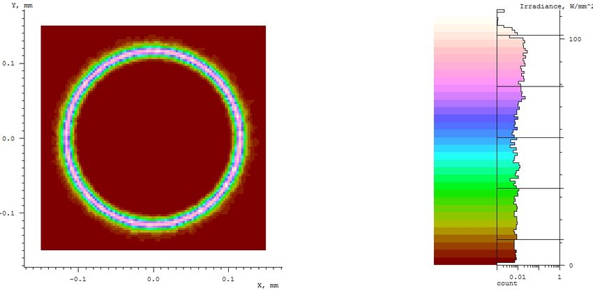
the material when it is cooling down. For instance, the PMMA dimensions shrink about 0.4% when solidifying, but the
volume close to the surface of the piece cools down faster than de interior. If the piece has uniform thickness (faceted
lenses, for example) the shrinkage is rather uniform. However, when thickness is non-uniform (continuous lenses case),
the thinner parts solidify completely while the interior of thicker parts still have to shrink, resulting in sinks and
deformations on the piece surface.
These two important problems lead us to choose solutions based on faceted optical elements such as Fresnel or TIR
lenses. Nevertheless faceted elements have manufacturing constrains that limit their geometry, mainly due to the draft
angle issue (see Figure 1). If single-piece manufacturing is desired, draft angles must have a positive value, higher than a
limit (typically >2º), in order to allow an unmolding process without frictions (these frictions can generate important lens
deformations). If dealing with domed-shape elements negative draft angles are required so we can have an acceptable
optical efficiency. In this case lenses must be built from several parts and join them all in a piece after having molded
each one of the single parts, implying higher manufacturing complexity and cost.
The novel solution proposed here allows for a single-piece manufacturing process with zero or negative draft angles
when designing faceted optical elements (mainly Fresnel lenses). These new designs are developed based on spiral
symmetry (each facet converting into the adjacent one after each turn), instead of the classical revolution symmetry
development (each facet describes a perfect ring after a whole turn around axis z). This freedom in draft angles value
presented by spiral symmetry designs maximizes optical efficiency and avoids the light incidence on the corner radii by
design.

                             2.   A BASIC SPIRAL EXAMPLE: FLAT FRESNEL LENS
Let us begin explaining our method with the most basic example of faceted refractive optical element: the flat Fresnel
lens. From now on we will work with the nomenclature and conventions introduced by concentration photovoltaics
(CPV) instead of illumination to make explanations easier, even though this design can be used for both applications.
2.1 Problem analysis
The classical Fresnel lens couples a plane input wavefront (with -z direction) with a spherical output wavefront with
origin in the focal plane center. For the flat Fresnel lens with spiral symmetry the input wavefront remains the same, but
the output one changes slightly: the output rays must reach now a circular ring centered in the focal plane. This output
wavefront will be helicoidal, presenting a vortex at its center (i.e. z axis, where there will be no light).
Using conservation of étendue theorem in two dimensions [2], a wavefront must verify:

                                    dE2 D = dxdp + dydq + dzdr = 0                                                      (1)

where p, q and r are the coordinates of the phase space corresponding to axis x, y and z, respectively. In the simple case
in which the receiver is a straight line (placed in the x axis, thus y=z=0), according to conservation of étendue (2) must
be satisfied:

                                              =
                                             dE2D  = 0
                                                  dxdp                                                                  (2)

In this situation, rays reaching the receiver will form an angle (β from now on) with respect to that straight line, being β
constant for a specific point of the receiver [3]. This means that every single ray impinging on the same point of the
receiver, it will be placed over the surface of a cone with circular base whose axis of symmetry will be the receiving line.
In our specific case in which the receiver is a circular ring, the line of symmetry of our cone will be the tangent line to
the ring at each one of its points. Therefore, and similarly to the straight line case, for each specific point of the receiver
every ray impinging on it will be placed on the surface of a cone forming an angle β with the tangent line of the receiver.
It is important to remark that angle β will vary with the position of the receiver chosen.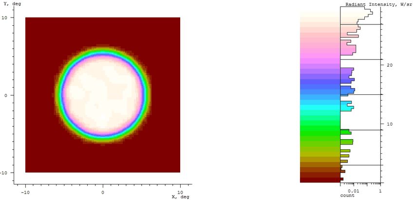
z

                                                                                                       y

                                                     θ       ρ0                         β
                                                                                                   γ
                                                                                         P(θ,γ)
                                        A0                        A

                       x

                             Figure 2 General scheme for the receiver ring, placed on z=0 plane.

Figure 2 shows a canonical situation for our spiral Fresnel lens design. Point A belonging to circular-shaped receiver
with constant radius ρ 0 has been chosen to illustrate what has been explained in the previous paragraph. As shown in the
figure, θ is the angle of point A position respect to initial point A 0 (placed on x axis). Calculating the corresponding β
value for point A, let us determine any point P in the 3D space just by knowing two angular parameters and a scalar one
P(θ,γ,d), instead of the classical Cartesian coordinate system P(x,y,z). θ determines the point on the receiver; γ
determines the corresponding line over the receiving cone; d indicates the physical distance between A and P (and so the
optical path length of raying going from P to A).
If we consider the skew invariant concept [4], defined for this situation by:

                                               h = n ρ0 cos β                                                            (3)

where n is the refractive index, the analytical development of our problem provides a double solution. In the first one
(with positive skew invariant h>0) the cone aperture is directed clockwise all along the receiver. In the second one
(h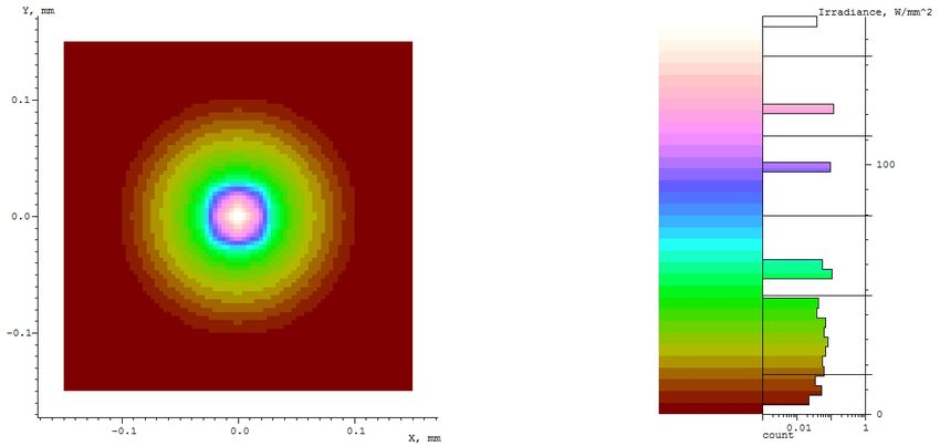
z

                                                                                                         ^t

                                                                                      ρ
                                                         z0                                                      P

                                                                                              ^
                                                                                              r
                                                                                                                -z^
                                                                                     d

                                                                               β
                                                          ρ0
                                                               A
            Figure 3 Scheme with generating spiral at z=z 0 plane and receiver at z=0 plane for a generic spiral point P
The shape of a particular 2D spiral is perfectly determined by defining the dependence, for any point belonging to it,
between its angular parameter θ and its distance to the spiral geometrical center, ρ. Figure 4 offers a 2D simplified
version of Figure 3 for an easier understanding of the analysis and easier identifying of the these parameters. We can
deduce from Figure 4:

                                                                                                         dρ
                                                                                          ^
                                                                                          t
                                                                                                   ^
                                                                                                   θ

                                                                                              α
                                                                                                  ρdθ

                                                       dθ       ρ
                                                                      α                            P
                                 ρ0
                                                         ρ·cosα
                                      A
                              Figure 4 View from above (projection on z=constant plane) of Figure 2
ρ0
sin α ( ρ ) =
ρ ρ0 d ρ dρ
tan arcsin = ⇒ ∫ dθ = ∫ (4)
dρ ρ ρ dθ ρ
tan α ( ρ ) = ρ ⋅ tan arcsin 0
ρ dθ ρ
Taking into account that almost the whole surface of lens will be composed by points for which approximation ρ 02.3 Lens constructions
We will build the whole lens starting by the generating spiral. In order to make the calculation easier, we will express all
the equations in terms of three parameters, as suggested in chapter 2.1: θ, γ, d (see Figure 2). In this way, we can reach
every single point in the whole 3D space, P(θ,γ,d) by applying:
) A (θ ) + d ⋅ r (θ , γ )
P (θ , γ , d= (7)
where every variable has already explained in chapter 2.1. Let us express all the variables in function of the desired
parameters:
A (θ ) = ( ρ0 cos θ , ρ0 sin θ , 0 )
r0 x sin β cos γ
) r0= r0 y = cos β
r (θ= 0= (8)
r sin β sin γ
0z
rx cos θ − sin θ 0 r0 x sin β cos γ cos θ − cos β sin θ
r (θ , γ ) = ry = sin θ cos θ 0 ⋅ r0 y = sin β cos γ sin θ + cos β cos θ
r 0 1 r0 z sin β sin γ
z 0
leading to the next expression:
x (θ , γ , d ) ρ0 cos θ + d ( sin β cos γ cos θ − cos β sin θ )
P (θ , γ , d ) =
y (θ , γ , d ) =
ρ0 sin θ + d ( sin β cos γ sin θ + cos β cos θ ) (9)
z (θ , γ , d ) d sin β sin γ
Now we will show that, to render our analysis even simpler, we can reduce point P dependence to just two parameters, θ
and γ. Even though the lens presents a spiral symmetry, since it couples an input wavefront with an output one, the lens
lower surface will be a Cartesian oval and thus an extra condition can be imposed. This condition is that of all normal
incident rays impinging on the lens aperture area and arriving to receiver must have constant value of optical path length.
In this way, using the eikonal function [5], L, we can obtain the optical path length between points A and P just by
subtracting both points’ eikonal function values. Using this extra condition and equation (6) we arrive to the following
expression of distance d, applicable to all the points belonging to lens lower surface (we just need to substitute β by its
value calculated with (6)):
( ρ0 ⋅θ ) + z0 2 ⋅ (1 − n sin β )
2
d (θ , γ , β ) = (10)
1 − n sin β sin γ
( ρ0 ⋅θ )
2
being n the material refraction index, and + z0 2 the value of d(θ,γ) when γ=π/2 (i.e. projection of line
between A and P on z=0 plane is tangent to generating circle in point A). If (6) is applied to (10) and (10) to (9) we can
finally obtain the desired expression P(θ,γ) for the points belonging to the lens lower surface.Now it can be deduced that the generating spiral line, placed on the plane z=z 0 (Figure 3), is obtained for all those points
satisfying P(θ, π/2). Starting by values γ= π/2 and θ=0 (i.e. β= π/2) we can vary progressively vary θ to higher values in
order to describe the whole generating spiral line. If we additionally vary γ as well, lens surface will also be built. In this
process, we will design the lens along “several turns” (ranging θ in more than one turn) and then we will cut our lens by
a vertical wall generated by a vertical extrusion of our spiral curve (creating the inactive facets). Figure 6 shows only
active facets, while Figure 7 shows our lens already cut, with the vertical facets dividing
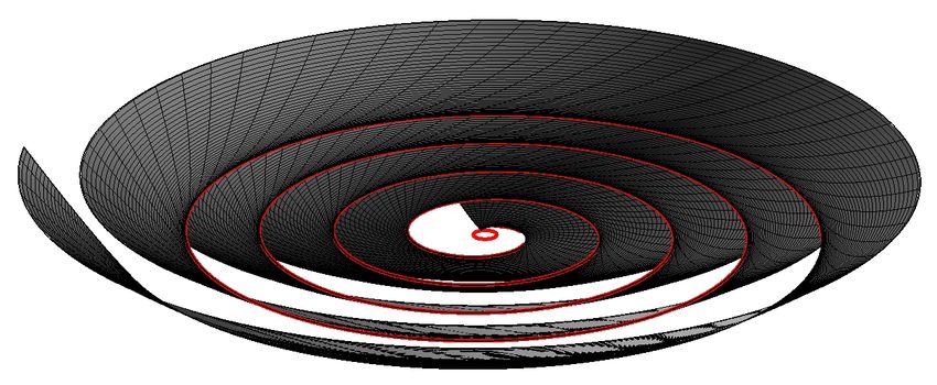
Figure 6 Several turns of the lens active surface (generating spiral in red color).
Figure 7 Lens already cut with vertical facets.
2.4 Simulation results
Raytrace simulations have been carried out in order to compare a flat Fresnel lens developed with spiral symmetry and a
classical flat Fresnel lens presenting revolution symmetry. We have chosen refractive index of PMMA and a f/1.5
parameter for both, while 2º draft angles have been taken into account for the revolution symmetry lens, which is a quite
realistic value. Efficiency results show a significant relative gain of 1.6% when working with the spiral design (91.9%optical efficiency for spiral design vs. 90.4% for revolution symmetry one, monochromatic λ=555nm simulations).
Figure 8 shows both illumination patterns, one spot-shaped and the other one ring-shaped.
Figure 8 Illumination diagram at the receiving plane, for square dimensions 0.15x0.15mm2. Top: revolution symmetry design.
Bottom: spiral symmetry design, with its characteristic ring-shaped illumination pattern.
3. SOME SPIRAL SYMMETRY COLLIMATOR DESIGNS
The flat Fresnel lens is a simple and canonical good example to explain our designing philosophy. Nevertheless we will
show here two more examples also developed with spiral symmetry, without a so detailed explanation of the design
procedure. The first of these examples is a dome-shaped Fresnel lens collimator with minimum angular range output,
while the second one is a similar collimator but presenting a +/- 30º output. Both designs’ simulations will be presented
for PMMA material for the lens.2.1 Dome-shaped Fresnel lens collimator with conical mirror
This device was first proposed in [6] using however a thick continuous lens. This device, in an ideal situation (point
source), can collimate completely a lambertian light source. Intensity patterns for both designs (continuous lens and
Fresnel lens with spiral symmetry) are almost identical but, as stated in the introduction, optical absorption in the first
case will be much higher than in the latter one (spiral design intensity shown in Figure 9). This is due to the obvious
difference between both lens thicknesses. Optical efficiency of this spiral design is 81.1% for monochromatic λ=555nm
simulation, and with a 100% reflectivity for the mirror.
Figure 9 Intensity pattern for spiral symmetry collimator
2.2 Dome-shaped Fresnel lens collimator with conical mirror, +/-30º output angle
This is a very similar design to that of previous section. Nevertheless there is a main difference in the output bundle
angle: while the previous design tried to maximize bundle collimation, this one reduces to a +/- 30º maximum angle the
output bundle. Figure 10 shows intensity results in the far field for this spiral symmetry design. Results are similar to
those that we would expect for a revolution symmetry design, with a neat +/-30º output bundle. Optical efficiency for
this case is quite similar to the previous design (polychromatic simulation with mirror perfect reflectivity): 78.4%.
Figure 10 +/-30º collimator intensity diagram in the far field.4. CONCLUSIONS
A novel designing method for faceted elements, especially for Fresnel lenses, has been described in this manuscript. The
designs explained along the text allow for an easy manufacturing process preventing from usual Fresnel lens fabrication
problems. These problems, as explained in the introduction, are draft angles and manufacturing of pieces based on
joining several parts.
The design method has been exposed in a neat and detailed way with a basic example as a flat Fresnel lens is. For this
spiral symmetry performance differences between it and its corresponding “revolution symmetry” version have been
described, explaining spiral version superiority. Other useful and interesting designs have been described, having based
them in the design philosophy stated to explain the flat Fresnel lens.
5. ACKNOWLEDGEMENTS
Authors wish to thank the Spanish Ministries MCINN (ENGINEERING METAMATERIALS: CSD2008-00066,
DEFFIO: TEC2008-03773, SIGMASOLES: PSS-440000-2009-30), MITYC (ECOLUX: TSI-020100-2010-1131, SEM:
TSI-020302-2010-65), the Madrid Regional Government (SPIR: 50/2010O.23/12/09,TIC2010 and O-PRO:
PIE/209/2010) and UPM (Q090935C59), and the EC, Spanish Ministry MITYC and C.A.M. under projects SSL4EU
(Grant agreement n º257550, FP7/2007-2013), V-SS and SMS-IMAGING (TSI-020100-2011-445 and 372, Plan Avanza
2011) and 4LL (PIE/468/2010), respectively, for the support given in the preparation of the present work.
6. REFERENCES
[1] Leutz, R., Suzuki, A., [Nonimaging Fresnel lenses], Springer-Verlag, Berlin (2001).
[2] Miñano, J. C., “Application of the conservation of étendue theorem for 2-D subdomains of the phase space in
nonimaging concentrators”, Appl. Optics, 23, 2021 (1984).
[3] Benítez, P., Mohedano, R., Miñano., J. C., “Design in 3D geometry with the Simultaneous Multiple Surface Design
method of Nonimaging Optics”, Proc. SPIE, 3781, 12 (1999).
[4] Chaves, J., [Introduction to nonimaging optics], CRC Press, Boca Raton, 420-429 (2008).
[5] Winston, R., Miñano, J. C., Benítez, P., [Nonimaging Optics], Elsevier-Academic Press, New York (2005).
[6] Chaves, J., Falicoff, W., Sun, Y., Parkyn, B., “Simple optics that produce constant illuminance on a distant target”,
Proc. SPIE 5529, 166 (2004).You can also read