Real-time Monitoring of Fluidized Bed Agglomerating based on Improved Adaboost Algorithm

Journal of Physics: Conference Series

PAPER • OPEN ACCESS

Real-time Monitoring of Fluidized Bed Agglomerating based on Improved
Adaboost Algorithm
To cite this article: Junqiu Pang and Zhong Zhao 2021 J. Phys.: Conf. Ser. 1924 012026

View the article online for updates and enhancements.

 This content was downloaded from IP address 46.4.80.155 on 26/08/2021 at 15:58

AIACT 2021 IOP Publishing
Journal of Physics: Conference Series 1924 (2021) 012026 doi:10.1088/1742-6596/1924/1/012026

Real-time Monitoring of Fluidized Bed Agglomerating based
on Improved Adaboost Algorithm

 Junqiu Pang1 and Zhong Zhao1,*
 1
 College of Information Science and Technology, Beijing University of Chemical
 Technology, Beijing, 100029, China.
 *
 corresponding author: zhaozhong@mail.buct.edu.cn

 Absctract: In order to to detect the polymer agglomeration in fluidized bed reactor (FBR), a
 method of real-time monitoring of agglomeration in fluidized bed polyolefin reactor based on
 voiceprint feature recognition is developed. First, the acoustic emission detection technology is
 applied to collect the acoustic signal generated by the polymer collision on the inner wall of
 FBR. Then, the voiceprint features of the collected acoustic signal are extracted with the Mel
 Frequency Cepstrum Coefficients (MFCC) and the Linear Prediction Cepstrum Coefficients
 (LPCC). To classify the extracted voiceprint features , an improved Adaboost algorithm is
 proposed to establish the real-time agglomeration classification model. Due to the introduction
 of cost factor and Gini index decision-making calculation to the Adaboost algorithm, the
 proposed improved Adaboost algorithm can classify unbalanced small samples with better
 accuracy and F-score index compared with the traditional Adaboost algorithm . The experiment
 results in a fluidized bed pilot plant have verified the effectiveness and feasibility of the proposed
 method.

1. Introduction
Currently, the repaid development of artificial intelligence technology provides more efficient and more
accurate method for fault diagnosis. [1-5] Nowadays, the main methods of machine learning include
support vector machines[6-11] (SVM) and artificial neural networks[12-15] (ANN). For example, a
support vector algorithm modified by genetic algorithm was applied in the fault diagnosis of fan blade
icing and exhibited good results[16]. However, the traditional support vector machines is one of the
weak classifiers for supervised learning, which is generally used for learning high-dimensional data.
More importantly, the support vector machines shows inferiority in the classification of multi-class data
sets[17] and poorer generalization ability. Besides, an algorithm based on the extreme learning was
proposed and applied in fault diagnosis for power plant, on the other hand, synthetic minority
oversampling technique (SMOTE) was used to processing the imbalanced data. Nevertheless, traditional
algorithms suffer various disadvantage, including small amount of sample information, fixed data
distribution and overfitting, and are not suitable for imbalanced data in the real industrial conditions.
 With the rapid development of speech recognition technology, speaker recognition based on
voiceprint feature extraction has made great progress. The speaker can be recognized by extracting the
individual voiceprint features from different speaker's speech signals. By analyzing the acoustic
emission signals in FBRs, different size particles collision can produce acoustic emission signals of
different frequencies. The acoustic emission signals in FBRs are relatively stationary in the normal

 Content from this work may be used under the terms of the Creative Commons Attribution 3.0 licence. Any further distribution
 of this work must maintain attribution to the author(s) and the title of the work, journal citation and DOI.
Published under licence by IOP Publishing Ltd 1

AIACT 2021 IOP Publishing
Journal of Physics: Conference Series 1924 (2021) 012026 doi:10.1088/1742-6596/1924/1/012026

production. In analogy with speech signals, the voiceprint feature recognition technology could be
applied to analyze the acoustic emission signals in FBRs.
 Owing to the great advantages, such as high precision, the Adaboost algorithm, which combines the
weak classifiers using the addition model, has been widely used in pattern recognition. However, such
algorithm shows low accuracy when dealing with imbalanced data, which deserves further research. In
actual industrial production, the number of samples in fault state is far less than the number of samples
in normal state, and the cost of wrong judgment of fault state is far greater than that of wrong judgment
of normal state.In this work, we propose a modified Adaboost algorithm with cost factor and Gini index,
which changes the basic decision rule of Adaboost algorithm. Combining the features of MFCC and
LPCC increases the difference of the data, thereby increasing the separability. The original Adaboost
algorithm and the modified Adaboost algorithm were both employed to monitor the agglomeration state
of the polyethylene in fluidized bed. The results reveal that the modified Adaboost algorithm shows
higher accuracy and superior efficiency. This work might provide a new strategy for learning algorithms.

2. Experimental section

2.1 Experimental device
 Fluidized bed

 AE sensor
 PC

 Data Acquisition Card

 Compressor Shield signal line

 Flowmeter

 Figure 1. Schematic illustration of experimental device.
As illustrated in Figure 1, the experimental device is consist of fluidized bed, AE sensor, signal shielded
line, data acquisition module and computer. The fluidized bed is a simplified simulation device of the
industrial fluidized bed, which is designed by Beijing Research Institute of Chemical Industry and can
simulate the hydrodynamic behaviour of the polyethylene in the industrial production process.

2.2 Acoustic vibration signals
In this work, PE particles with three different size (1, 2 and 5 mm) were investigated. Under the similar
condition (air velocity and bed weight) of industrial production process, the time-domain acoustic
vibration signals of PE particles in the fluidized bed were collected using the acoustic emission
technology and displayed in Figure 2.

 Figure 2. The time-domain acoustic vibration signals of various PE particles.

 2

AIACT 2021 IOP Publishing
Journal of Physics: Conference Series 1924 (2021) 012026 doi:10.1088/1742-6596/1924/1/012026

2.3 The extraction of LPCC
In the Cepstrum domain, Linear Prediction Cepstrum Coefficient (LPCC) is the expression of Linear
Prediction Cepstrum Coefficient (LPC) [18-20] Figure 3 shows the extraction process of LPCC feature.

 Figure 3. Schematic illustration of the extraction process of LPCC [20].
 The LPCC is a cepstrum coefficient that derived from the linear prediction model and the
corresponding LPC coefficient, which can be directly determined according to formula (1).
 ĥ (1)=a1
 i
 ĥ (n)=an + ∑n-1 ̂
 i=1 (1- n) ai h(n-i) 1p
 {
where, is the LPC coefficient, ℎ̂( ) is the LPCC coefficient. According to the previous work, [19] 
can be obtained by using auto-correlation method and co-correlation method. In this work, 200 samples
of each size (1, 2 and 5 mm) were investigated. Figure 4 displays the as- extracted LPCC features of the
acoustic vibration signals, as it shown, the LPCC features at 1-200 frames, 200-400 frames and 400-600
frames are corresponding to the three different PE particles. Notably, there LPCC features are extracted
in 8 different dimensions.

 Figure 4. The LPCC features of various acoustic vibration signals.

2.4 The extraction of MFCC

 Figure 5. Schematic illustration of the extraction process of MFCC.
 Figure 5 illustrates the extraction process of the MFCC features. As it shown, the energy spectrum
(E(k)) can be determined according to the formula (2-3).
 X (k ) = FFT [ x(m)] (2)
 E (k ) = [ X (k )]2 (3)

 3

AIACT 2021 IOP Publishing
Journal of Physics: Conference Series 1924 (2021) 012026 doi:10.1088/1742-6596/1924/1/012026

where, x(m) is the time series of a single frame signal, X(k) is the frequency spectrum of the
corresponding single frame signal. By calculating the energy passing through the Mel triangle filter [32]
and performing discrete cosine transform (DCT) on the as-processed signal, the MFCC features can be
determined according to the discrete cosine transform (formula 4) , which are shown in Figure 6.
 2 πl(2m+1)
 MFCC(i,l)=√M ∑M-1
 m=0 log[S(i,m)] cos ( 2M
 ) (4)

where, ( , )is the energy of the Mel filter.

 Figure 6. The MFCC features of various acoustic vibration signals.
 According to the Figure 4 and 6 as well as the discussions of the LPCC and MFCC features, we can
find that these features are stable and separable. In each dimension, the characteristic values of the
different classes of polyethylene voice print fluctuate is around a certain value, which would provide
possibility for voiceprint recognition in this experiment.

2.5 Adaboost algorithm and modified Adaboost algorithm
Adaboost algorithm is a representative boosting algorithm, which can realize the formation of a strong
classifier by continuously modifying the weight of training samples. Typically, by increasing the weight
of misclassified samples and decreasing the weight of well-classified samples in the process of each
iteration, the misclassified samples can be furthest emphasized, thus, a strong classifier can be obtained
after the weighted voting of multiple weak classifiers. The original Adaboost algorithm are listed as
followed.
 (1) Input.
 A training set X is consist of samples (x1 ,y1 ) (x2 ,y2 ) …(xn ,yn ), where x is the sample feature (x is
the four-dimensional feature value in this experiment), y is the sample label.
 (2) Initialize the weight distribution value of the training data.
 1
 D1 =(ω11 ,……,ω1i ,……,ω1N ),ω1i = N (5)
where, 1 is the weight of each sample for the first iteration, ω11 is the weight of the first sample for the
first iteration, and N is the sample number.
 (3) For M iterations. m=1, 2... M, m is the iterations.
 (a) Use the training set with the weight distribution of to learn and find the basic
classifier ( ), the output value of which is {1,-1}.
 (b) Calculate the classification error rate (em ) of ( ). Lower value of em leads to greater role of
the basic classifier in the final classifier.

 4

AIACT 2021 IOP Publishing
Journal of Physics: Conference Series 1924 (2021) 012026 doi:10.1088/1742-6596/1924/1/012026

 em =P(Gm (xi )≠yi ) ∑N
 i=1 ωmi I(Gm (xi )≠yi ) (6)
where, the value of I(Gm (xi )≠yi can be 0 or 1. If the value if 0, the classification is correct.
 (c) Calculate the weight coefficient ( αm ) of ( ) .
 1 1-em
 αm = 2 ln em
 (7)

where, the value of should be less than 0.5 and the value of am increases with the decreasing of the
 .
 Currently, the classifier can be indicated as:
 f(x)= Gm (x)
 (8)
 (d) Update the sample weight distribution of the training set and use for the m+1 iteration.
 Dm+1 =(ωm+1,1 ,ωm+1,2 ,…ωm+1,i ,…,ωm+1,N ) (9)
 , 
 ωm+1,i = zm
 exp (-am yi Gm (xi )) , i=1,2,…,N (10)

 Zm = ∑N
 I=1 ωmi exp (-am yi Gm (xi )) (11)

where, Zm is normalization coefficient.
 For two classifications, the output value of the weak classifier Gm (x) is {-1,1}, and the value of is
{-1,1}, thus, yi Gm (x)>0 and yi Gm (x)

AIACT 2021 IOP Publishing
Journal of Physics: Conference Series 1924 (2021) 012026 doi:10.1088/1742-6596/1924/1/012026

 The quantity ratio of the three different samples is m: n: q (m, n and q correspond to the normal
fluidization state, micro-agglomeration and serve-agglomeration, respectively, and m>n, m>q), then the
cost factor ( ) can be estimated using formula (15).
 θ
 m
 θ
 θi = { n (15)
 m
 θ
 q

where, the value of θ is customized. (2) Initialize the sample weights.
 θ
 D1 =(ω11 ,……,ω1i ,……,ω1N ),ω1i = ∑ iθ (16)
 i i

 Thus, the small class samples have greater initial weight and would show greater importance in the
classification.
 (3) Find the basic classifier Gm(x) by looking for the optimal classifier.
 (4) Calculate the classification error rate em of Gm(x) using formula (17).
 em =P(Gm (xi )≠yi ) ∑N
 i=1 ωmi I(Gm (xi )≠yi ) (17)
 (5) Calculate the weight coefficient αm of Gm(x).
 1 1-em
 αm = 2 ln em
 (18)

 (6) Calculate the GINI index of each sample.
 GINI=1- ∑i Pi 2 (19)
 (7) Update the sample weight distribution of the training set.
 ∙ℯ − ( − )+ 
 ωm+1,i = , zm
 , yi Gm (x)>0
 { (20)
 ⋅ℯ + 
 
 ωm+1,i = , z , yi Gm (x) , μ is an adjustment parameter.
 (8) Weighted combination of the basic classifiers.
 Gm (x)=sign(f(x) )=sign[ ∑M
 m=1 αm Gm (x) ] (21)
 As can be seen in formula (20), if the classification is correct, the weight of the sample with high
 decreases more slowly than the sample with low , and the sample with a higher Gini index shows a
lager weight change. On the other hand, if the classification is incorrect, the weight of the sample with
high shows larger increasement, and the sample with a higher Gini index displays a large weight.

3. Results and discussion
According to the principle component analysis (PCA) algorithm, the eight-dimensional LPCC and
MFCC features can be changed into a four-dimensional LP-MFCC features. As shown in Figure 7, the
LP-MFCC features show the superior stability, better separability and inferior complexity, resulting in
prevented over-fitting and improved computational efficiency.

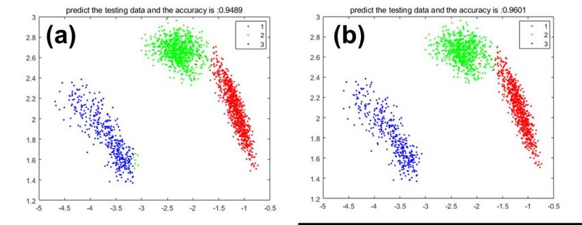
 6

AIACT 2021 IOP Publishing
Journal of Physics: Conference Series 1924 (2021) 012026 doi:10.1088/1742-6596/1924/1/012026

 Figure 7. Four-dimensional LP-MFCC features of the acoustic vibration signals.
 The LP-MFCC features of the PE with three different states are used as the inputting dataset, of
which 80% is training sets and 20% is testing set, and three different PE are classified using original
Adaboost algorithm and modified Adaboost algorithm, then, the predicted results of 600 testing sets
are exhibited in Figure 8 respectively. As shown in Figure 8, 1.2.3 respectively corresponding to the
distribution of the predicted results of PE in three states. there are many errors in the prediction of
category 3 in Figure 8a, which category 3 is mispredicted as category 2, while the prediction accuracy
in Figure B is significantly higher than that in Figure A, the modified Adaboost algorithm presents
higher accuracy of 0.9601, demonstrating its superiority. However, there are some arguments that larger
amount of imbalanced data would lead to the higher accuracy, thus, only the accuracy cannot elucidate
the advantage of the modified algorithm. To address this issue and obtain an algorithm with great
practical significance, the F-score (formula 22) was employed as a model evaluation standard.

 Figure 8. The classification accuracy of the (a) original Adaboost algorithm and (b) the modified
 Adaboost algorithm.
 2*pre*recall
 F-score= (22)
 pre+recall

 Table 1-3 display the F-score of the original Adaboost algorithm and the modified Adaboost
algorithm.
 When the normal fluidization state is positive, and the micro-agglomeration and the severe-
agglomeration state are negative, the results are shown in Table 1.

 Table 1. F-score when the normal fluidization state is positive.
 index Adaboost Algorithm Modified Adaboost Algorithm

 7

AIACT 2021 IOP Publishing
Journal of Physics: Conference Series 1924 (2021) 012026 doi:10.1088/1742-6596/1924/1/012026

 pre 0.8666 0.9452
 recall 0.9285 0.8625
 F-score 0.8964 0.9020
 When the micro-agglomeration state is positive, the normal fluidization and the severe-
agglomeration state are negative, the results are shown in Table 2.

 Table 2. F-score when the micro-agglomeration state is positive.
 index Adaboost Algorithm Modified Adaboost Algorithm
 pre 0.9714 0.9330
 recall 0.9023 0.9897
 F-score 0.9356 0.9605
 When the severe-agglomeration state is positive, the normal state and the micro-agglomeration state
are negative, the results are shown in Table 3.

 Table 3. F-score when severe-agglomeration state is positive.
 index Adaboost Algorithm Modified Adaboost Algorithm
 pre 0.9428 0.9677
 recall 0.9428 0.9961
 F-score 0.9428 0.9816
 As shown in Table 1, 2 and 3, the modified Adaboost algorithm present higher F-score in the 3
different state of polyethylene (normal, micro-agglomeration and severe agglomeration), especially for
the detection of micro-agglomeration and severe-agglomeration states. Therefore, compared with
original Adaboost algorithm, the modified Adaboost algorithm can effectively improve the efficiency
of failure prediction.

4. Conclusions
In this work, a modified Adaboost algorithm has been proposed, which significantly improved the
monitoring efficiency and accuracy of agglomeration faults in the industrial production process of
polyethylene. Typically, the pre-processing process and the combination of LP-MFCC features
improved the stability and the separability of the acoustic vibration signals, resulting in excellent
classification accuracy and efficiency. Furthermore, the introduction of cost parameter and the Gini
index effectively increased the classification accuracy and efficiency of imbalanced data. Such new
algorithm shows great perspective in industrial application.

Acknowledgements
This work was supported by Collaborative Innovation Project of Chaoyang District (ZK20170007).

Notes and references
[1] F. A. N. Fernandes and L. M. F, Journal of Applied Polymer Science, 2001, 81, 321-332.
[2] M. L. Mastellone, F. Perugini, M. Ponte and U. Arena, Polymer Degradation and Stability, 2002,
 76, 479-487.
[3] O. Vahidi and M. Shahrokhi, Indian Journal of Chemical Technology, 2018, 25, 21-30.
[4] H. L. Zhu, Y. S. Zhang, M. Materazzi, G. Aranda, D. J. L. Brett, P. R. Shearing and G. Manos,
 Fuel Processing Technology, 2019, 190, 29-37.
[5] K. C. Xie and M. J. Zhao, Energy Sources, 2003, 25, 1073-1081.
[6] Q. Yu, W. Li, H. Zhang and D. Yang. Sustainability, 2020, 12, 6203.

 8

AIACT 2021 IOP Publishing
Journal of Physics: Conference Series 1924 (2021) 012026 doi:10.1088/1742-6596/1924/1/012026

[7] B. Pan, H.F. Duan, S. Meniconi and B. Brunone, Mechanical Systems and Signal Processing,
 2021, 146, 107056.
[8] M. M. Dubrovin and V. A. Belyaev, Instruments and Experimental Techniques, 2002, 45, 548-
 549.
[9] J. Sun, H. Zuo, P. Liu and Z. Wen, Measurement Science and Technology, 2013, 24, 125107.
[10] X. Chen, Y. Zhang and J. Zhang, J. Chem. Phys., 2005, 122, 184105.
[11] A. Al-Ali, D. Dean, B. Senadji, V. Chandran and G. Naik, IEEE Access, 2017, 5, 15400-15413.
[12] O. C. Ai, M. Hariharan, S. Yaacob and L. S. Chee, Expert Systems with Applications, 2012, 39,
 2157-2165.
[13] Q. Li, Y. Yang, T. Lan, H. Zhu, Q. Wei, F. Qiao, X. Liu and H. Yang, IEEE Access, 2020, 8,
 48720-48730.
[14] J. Wang, J. Wang and Y. Weng, Integration-the Vlsi Journal, 2002, 32, 111-131.
[15] Q. Meng and Y. Peng, Physics Letters A, 2007, 370, 465-470.
[16] C. Bai and H. Li, Open Mathematics, 2018, 16, 1037-1047.
[17] H. I. Lee, Y. H. In, S. Y. Jeong, J. M. Jeon, J. G. Noh, J. S. So and W. Chang, Letters in Applied
 Microbiology, 2014, 59, 9-16.

 9