Objective and algorithm considerations when optimizing the number and placement of turbines in a wind power plant
←
→
Page content transcription
If your browser does not render page correctly, please read the page content below

Wind Energ. Sci., 6, 1143–1167, 2021
https://doi.org/10.5194/wes-6-1143-2021
© Author(s) 2021. This work is distributed under
the Creative Commons Attribution 4.0 License.

        Objective and algorithm considerations when optimizing
            the number and placement of turbines in a wind
                              power plant
                       Andrew P. J. Stanley, Owen Roberts, Jennifer King, and Christopher J. Bay
            National Renewable Energy Laboratory, National Wind Technology Center, Boulder, CO 80303, USA
                                Correspondence: Andrew P. J. Stanley (pj.stanley@nrel.gov)

                                    Received: 2 March 2021 – Discussion started: 18 March 2021
                           Revised: 27 May 2021 – Accepted: 29 July 2021 – Published: 9 September 2021

       Abstract. Optimizing turbine layout is a challenging problem that has been extensively researched in the liter-
       ature. However, optimizing the number of turbines within a given boundary has not been studied as extensively
       and is a difficult problem because it introduces discrete design variables and a discontinuous design space. An
       essential step in performing wind power plant layout optimization is to define the objective function, or value,
       that is used to express what is valuable to a wind power plant developer, such as annual energy production, cost
       of energy, or profit. In this paper, we demonstrate the importance of selecting the appropriate objective func-
       tion when optimizing a wind power plant in a land-constrained site. We optimized several different wind power
       plants with different wind resources and boundary sizes. Results show that the optimal number of turbines varies
       drastically depending on the objective function. For a simple, one-dimensional, land-based scenario, we found
       that a wind power plant optimized for minimal cost of energy produced just 72 % of the profit compared to the
       wind power plant optimized for maximum profit, which corresponded to a loss of about USD 2 million each
       year. This paper also compares the performance of several different optimization algorithms, including a novel
       repeated-sweep algorithm that we developed. We found that the performance of each algorithm depended on the
       number of design variables in the problem as well as the objective function.

1   Introduction                                                   prove, and wind energy capacity and market penetration are
                                                                   to increase even further (U.S. Energy Information Adminis-
Wind energy provides several advantages to the sustainable         tration, 2019).
energy grid of the future. Wind turbines produce minimal              Because of economies of scale, utility-scale wind turbines
carbon dioxide or other air pollution, require no external fuel    are deployed in groups. This provides reduced cabling costs,
during operation, and require little water throughout their        easier construction and maintenance, and reduced land re-
lifetime (Meldrum et al., 2013). Additionally, wind plants         quirements. However, building turbines close together also
have an energy payback time of less than a year and can            introduces some challenges. One of these challenges is wake
produce energy in an economically efficient manner (Raz-           interaction between turbines. A wind turbine removes ki-
dan and Garrett, 2017; Vestas, 2020). In fact, wind energy         netic energy from the air around it and converts this energy
has been a central focus of research and development in past       to electricity, creating a wake of slow-moving and turbulent
decades such that, currently, wind is one of the cheapest          wind behind it. When turbines are built close together, their
sources of energy available (Lazard, 2018). Because of its         wakes can reduce the amount of energy available in the wind,
many benefits, but in large part due to the economic drivers,      causing downstream turbines to produce less energy as a re-
wind energy installations have grown throughout the world          sult. One way to reduce wake interactions between turbines
as has the relative share of energy produced by wind. In           is through wind power plant layout optimization. This op-
coming years, wind energy technology is projected to im-           timization process involves determining the number of tur-

Published by Copernicus Publications on behalf of the European Academy of Wind Energy e.V.
1144                                                                            A. P. J. Stanley et al.: Objective and algorithm

bines to build in a wind power plant and their locations in or-    and Espiritu, 2011; Moorthy and Deshmukh, 2015). Addi-
der to reduce wake interactions and maximize performance.          tionally, some applied a similar methodology to optimiz-
Finding an optimal wind power plant layout is a challenging,       ing turbine number and layout at real geographical locations
nonconvex problem with many interacting design variables.          (Şişbot et al., 2010; Khanali et al., 2018). The vast majority
It is difficult to solve this problem without mathematical opti-   of these more recent studies kept the same general optimiza-
mization tools because it often requires not-so-obvious trade-     tion strategy, performed by dividing the wind power plant do-
offs to reach a solution.                                          main into a grid that defines potential turbine locations and
    Appropriate methods of determining turbine locations           using some optimizer to determine the best layouts.
within a wind power plant have been intensively studied, and           Selecting the appropriate optimization methodology is a
researchers have demonstrated several methods that can be          vital part of the wind power plant layout optimization process
used to effectively optimize a wind power plant layout. The        because it determines the quality of the final solution as well
literature demonstrates a preference for gradient-free opti-       as the required computational expense. In addition to the op-
mization methods applied to wind power plant layout opti-          timization algorithm, a critical step is to appropriately select
mization, and different studies showed success using genetic       the objective function. For wind power plant layout optimiza-
algorithms (Grady et al., 2005; Mittal, 2010; Abdelsalam and       tion studies, objectives that are often considered are annual
El-Shorbagy, 2018), greedy algorithms (Song et al., 2015;          energy production (AEP) or cost of energy (COE). With a
Chen et al., 2016), particle swarm methods (Pookpunt and           fixed number of turbines, the objective may not have much
Ongsakul, 2013; Hou et al., 2015), and random search (Feng         of an effect on the final solution. However, when the number
and Shen, 2013, 2015) to determine improved wind power             of turbines is also being optimized, the objective function can
plant layouts (Hou et al., 2019). A common layout optimiza-        have a profound effect on the final optimized layout. For one
tion method is to divide the wind power plant domain into          set of optimizations discussed in Sect. 6.4, the optimal num-
a grid that defines possible turbine locations (at the center      ber of turbines ranges from 15–54, and the annual costs range
of the grid cells or at the intersections of the lines). One of    from USD 6.75 million to USD 21.96 million, depending on
the previously mentioned optimization methods is then used         if the plant was optimized for AEP, COE, or profit.
to determine at which of the predefined locations a turbine            For this paper, we studied two specific considerations in
should be placed. In more recent years, some studies also          optimizing the number of turbines and their layout in a wind
showed success optimizing wind power plant layouts with            power plant. First, we determined how different objective
gradient-based methods (Thomas and Ning, 2018; Stanley             functions alter the optimized number of wind turbines and
and Ning, 2019a; Baker et al., 2019). This type of optimiza-       their layout in a wind power plant. Li et al. (2017) began
tion requires a continuous design space and computationally        to explore this sensitivity with multi-objective optimization
or analytically provided gradients that increase the complex-      of wind farm layout and turbine number, considering AEP
ity of the problem formulation. However, the computational         and COE. As part of their paper, these authors examined how
expense required for gradient-based optimization scales fa-        different formulations of the COE definition affected the fi-
vorably with increasing numbers of design variables com-           nal solutions. Balasubramanian et al. (2020) also mention the
pared to gradient-free methods for which the computational         importance of appropriately defining the objective for wind
expense scales very poorly.                                        farm layout optimization. For our paper, we included an em-
    Layout optimization studies are almost always performed        pirically based cost model and compared three different ob-
assuming that the number of turbines in the wind power plant       jectives in our single objective optimization formulation to
is previously known. Determining the optimal number of tur-        further understand the sensitivity of wind farm layout and
bines in a wind power plant is a much more difficult problem       turbine number to the objective. Second, we tested using dif-
to solve because it requires the optimization of at least one      ferent problem formulations and optimization algorithms in
integer design variable or a discontinuous design space. Al-       finding a solution. In past research on wind farm layout opti-
though it has not been discussed in the literature as much as      mization, there was a wide variety of algorithms and problem
layout optimization determining turbine placement, optimiz-        formulations used, with little consensus on which strategies
ing the number of turbines in a wind power plant has also          are the best (Shakoor et al., 2016; Baker et al., 2019; Hou
been researched in previous studies. Mosetti et al. (1994)         et al., 2019; Balasubramanian et al., 2020). For this paper,
first addressed this issue when they divided a wind power          we specifically studied how different algorithms performed
plant domain into 100 square cells as candidate turbine lo-        depending on the objective and the size of the optimization
cations and then used a genetic algorithm to determine the         problem. We compared a genetic algorithm and a greedy al-
optimal number of turbines and at which of the potential lo-       gorithm in a gridded wind power plant domain, two com-
cations they should be placed. Since this seminal paper was        monly used wind power plant optimization methods, as well
published, many other researchers have proposed improve-           as a genetic algorithm with the boundary-grid method and a
ments to Mosetti’s methodology and were able to find im-           new repeated-sweep algorithm in a gridded domain.
proved results, mostly by using new and better optimizers              The rest of this paper is outlined as follows: Sect. 2
(Grady et al., 2005; Zergane et al., 2018; Ituarte-Villarreal      presents the wake model we used in this paper and the rel-

Wind Energ. Sci., 6, 1143–1167, 2021                                                 https://doi.org/10.5194/wes-6-1143-2021
A. P. J. Stanley et al.: Objective and algorithm                                                                            1145

evant turbine parameters; Sect. 3 presents the power models,      direction. The distributions σz and σy are defined as follows:
cost models, and how they are combined to form the three ob-
jective functions we explored in this paper; Sect. 4 describes    σz      (x − x0 ) σz0
                                                                     = kz          +
the different sets of design variables we used to define the      D          D       D
locations of wind turbines; Sect. 5 explains the optimization     σy      (x − x0 ) σy0
                                                                     = ky          +    ,
algorithms we used in this paper; Sect. 6 presents and dis-       D          D       D
cusses the results from our optimizations; Sect. 7 explains
                                                                  where x − x0 is the downstream distance between the point
the empirical considerations of this work and gives a gen-
                                                                  of interest x and the onset of the far wake x0 , σy0 and σz0
eral overview of the different scenarios we considered; and
                                                                  refer to the wake width at the start of the far wake, ky defines
Sect. 8 contains our conclusions from this work.
                                                                  the wake expansion in the lateral direction, and kz defines
                                                                  the wake expansion in the vertical direction. The length of
2   Wake model                                                    the near wake is defined as follows:
                                                                                        √
The wind speed downstream of a turbine is reduced because         x0          cos γ (1 + 1 − CT )
                                                                      =√                    √            ,
turbines extract energy from the flow and from the complex         D        2[4αI + 2β(1 − 1 − CT )]
physics of the wakes they produce. In this paper, the desir-
ability of the wind power plants we examined was depen-           where α = 0.58, β = 0.077, and I is the incoming stream-
dent, to a large extent, on energy production. This energy        wise turbulence intensity for which we used a freestream tur-
production is a function of the wind speeds throughout the        bulence of 6 % and the Crespo-Hernández model for wake
wind power plant. To calculate the wind speeds to be used         added turbulence (Crespo and Hernández, 1996). The vari-
in turbine power calculations, we used an analytic Gaussian       ables σy0 and σz0 are given in the following equations:
wake model (Bastankhah and Porté-Agel, 2016; Abkar and                    r
                                                                  σz0   1      uR
Porté-Agel, 2015; Niayifar and Porté-Agel, 2016). The wake            =
calculations were performed using FLOw Redirection and             D    2 U∞ + u0
Induction in Steady State (FLORIS), which is a computa-           σy0   σz0
                                                                      =     cos γ ,
tionally inexpensive, controls-oriented tool to calculate the      D    D
steady-state flow field in a wind power plant (National Re-       where uR and u0 are defined with the thrust coefficient CT
newable Energy Laboratory, 2021). We include a brief de-          and the freestream wind speed U∞ :
scription of the Gaussian wake model in this paper but, for
more details, refer to the original model paper (Bastankhah       uR        CT
and Porté-Agel, 2016).                                               =      √
                                                                  U∞   2(1 − 1 − CT )
   Using the Gaussian wake model, the velocity of the wake        u0   p
behind a turbine is computed with the following analytical           = 1 − CT .
                                                                  U∞
expressions:
                                                                  For this study, ky and kz are set to be equal, meaning the wake
u(x, y, z)               2   2         2   2                      expands at the same rate in the lateral and vertical directions.
           = 1 − Ce−(y−δ) /2σy −(z−zh ) /2σz
  U∞                                                              These wake spreading parameters ky and kz are defined as
                 s                                         (1)    follows:
                      D 2 CT cos(γ )
        C = 1− 1−                    ,
                          8σy σz                                  kz = ky = ka I + kb ,

where u is the velocity at a desired location (x, y, z), where    where ka = 0.38 and kb = 0.004. In the case of interacting
x, y, and z refer to the streamwise, cross-stream, and vertical   wakes, the wake deficits were combined using the traditional
coordinates, respectively, U∞ is the freestream velocity, C       sum of squares method (Katić et al., 1986). Equation (1)
is the velocity deficit at the wake center, y − δ is the cross-   defines the wind speed, u, at a single desired point. To de-
stream distance between the point of interest and the wake        termine the average rotor wind speed used to calculate the
center (where δ is the y coordinate of the wake center and        power production of a wind turbine, we averaged the wind
is assumed to extend straight back from the turbine creating      speeds sampled at nine locations across the swept rotor area,
the wake if the turbine is not yawed), z − zh is the vertical     which is the default in FLORIS. These nine sample locations
distance between the point of interest and the wake center        are shown in Fig. 1.
(where the wake center is assumed to be at zh , the hub height       For this study, we used a 2.5 MW turbine definition. The
of the turbine creating the wake), D is the rotor diameter, CT    turbine parameters are shown in Table 1, and the power and
is the thrust coefficient, γ is the rotor yaw angle (which is     thrust coefficient curves, as well as the power curve, are
assumed to be 0 in this paper), σy defines the wake width         shown in Fig. 2. As seen in the power curve, the rated wind
in the y direction, and σz defines the wake width in the z        speed is near 10 m s−1 .

https://doi.org/10.5194/wes-6-1143-2021                                                   Wind Energ. Sci., 6, 1143–1167, 2021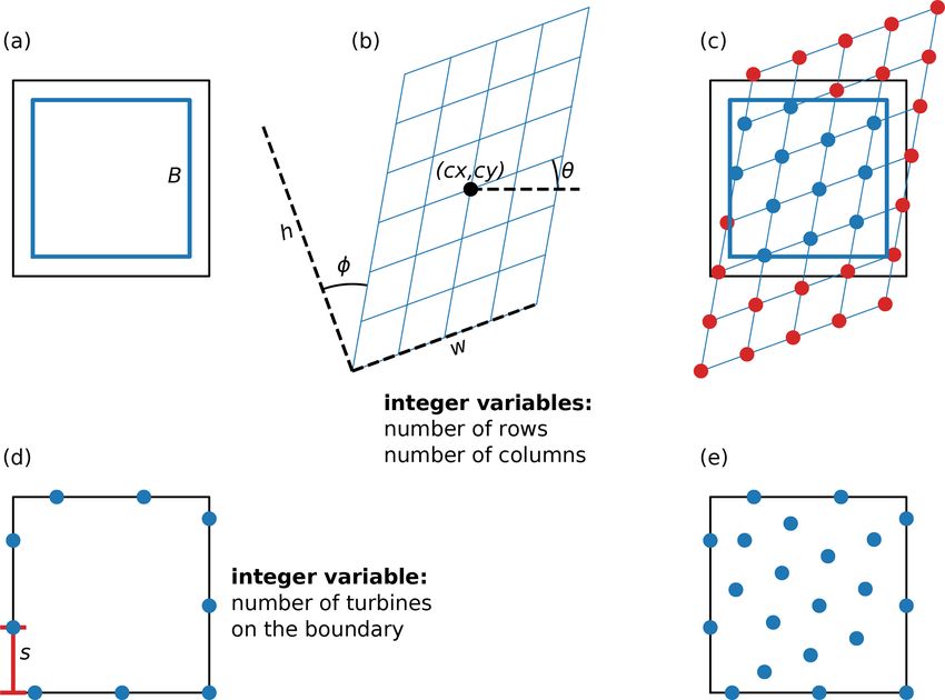
1146                                                                                A. P. J. Stanley et al.: Objective and algorithm

                                                                      Figure 2. (a) CP and CT curves for the 2.5 MW turbine used in this
                                                                      study. (b) The power curve for this same turbine.
Figure 1. The nine locations at which the wind speeds are calcu-
lated across a wind turbine rotor. D represents the rotor diameter,
while H is the turbine hub height. The effective turbine wind speed   per wind direction, Pf is the power production of the wind
is determined as the average of the wind speed at each of these       power plant, φ is the wind direction, U is the wind speed, and
points.                                                               fi and fj are the frequency of wind associated with a given
                                                                      direction and speed.
Table 1. Wind turbine parameters.                                        The power of an individual turbine is calculated as fol-
                                                                      lows:
                    rated power           2.5 MW                          1
                    rotor diameter        117.8 m                     Pt = ρAV 3 CP (V ),
                                                                          2
                    hub height            88 m
                                                                      where Pt is the power produced by a single turbine; ρ is the
                                                                      density of air, which we assumed is 1.225 kg m−3 ; A is the
3     Objective functions                                             rotor swept area of the wind turbine; CP is the power co-
                                                                      efficient of the turbine; and V is the effective wind speed
For this paper, we explored three different objective functions       across the swept area, which for this paper was calculated
in our wind power plant optimizations: (1) AEP, (2) COE,              with the wake model discussed in Sect. 2. When there is
and (3) annual profit. In this section, each objective function       a variable number of turbines, one can expect that a wind
is described in detail. We acknowledge that the models we             power plant optimized for maximum AEP will have many
used in this paper are simple. These simplified models are            turbines spaced close together, filling the available land. If
sufficient for this demonstration and investigation into vary-        there are no penalties for costs considered in the optimiza-
ing results from different objectives; however, more detailed         tion, additional turbines will lead to an improved objective,
models can be easily included, depending on the use case and          even if they are extremely inefficient and operate with high
data available.                                                       wake interference.

3.1    Annual energy production                                       3.2   Cost of energy

AEP is a standard objective in wind power plant optimization          In some optimization problems, AEP may not be an appro-
(Pérez et al., 2013; Gebraad et al., 2017; Thomas and Ning,           priate objective as it does not account for the added cost or
2018). For problems where the value of energy produced by             complexity required to achieve gains in AEP. An example
the wind power plant is fixed throughout its lifetime and in-         of this is wind turbine blade design, for which an increase in
dependent of the time of day, and where the project cost re-          AEP comes at the cost of additional mass and, therefore, cost.
mains constant or is not an important consideration, AEP is a         In a situation like this, it may be more appropriate to perform
reasonable objective. AEP optimization simply aims to max-            multi-objective optimization or include both AEP and cost
imize the energy production. For example, AEP is a common             into a single objective. COE is another common metric used
objective for wind power plant layout optimization where the          in wind power plant design that captures both energy produc-
turbine number and design are fixed. Typically to calculate           tion and costs (Chen and MacDonald, 2014; Fleming et al.,
AEP, the wind directions and wind speeds are grouped into             2016; Stanley and Ning, 2019a). We calculated COE as a
discrete bins in order to numerically calculate the integral:         combination of costs divided by the AEP:

              nd X
                 ns                                                           cost
              X                                                       COE =
AEP = 8760               Pf (φi , U (φi )j )fi fj ,                           AEP
              i=1 j =1                                                cost = FCR(TCC + BOS) + O&M,

where 8760 is the number of hours in a year, nd is the number         where FCR is the annual fixed charge rate, which we as-
of wind direction bins, ns is the number of wind speed bins           sumed was 9.7 % (Previsic, 2011); TCC is the turbine capital

Wind Energ. Sci., 6, 1143–1167, 2021                                                     https://doi.org/10.5194/wes-6-1143-2021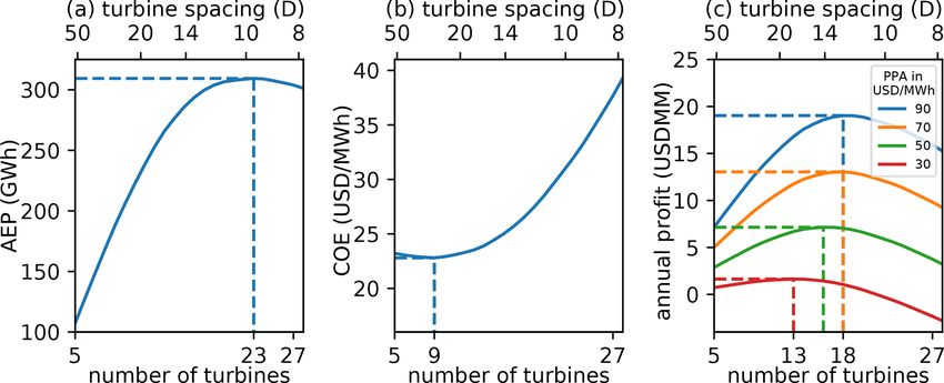
A. P. J. Stanley et al.: Objective and algorithm                                                                                    1147

Figure 3. The balance of station (BOS) cost model (per kilowatt of
installed wind power plant capacity) as a function of the total power
plant capacity (Key et al., 2020).                                      Figure 4. A square wind power plant that has been discretized with
                                                                        a square grid for wind turbine number and layout optimization.

cost, which we assumed is USD 829 kW−1 of plant capacity
(Wiser et al., 2020); O&M is the operation and maintenance              though we varied this constant to study its effect during dif-
cost, which we assumed is USD 44 kW−1 of plant capacity                 ferent optimizations. One should expect that a wind power
per year (Stehly and Beiter, 2020); and BOS is the balance              plant optimized to maximize profit would have fewer tur-
of station cost. For this paper, we created a simple relation of        bines than one optimized for maximum AEP, but more tur-
BOS costs as a function of the installed wind power plant ca-           bines than one that is optimized for minimum COE. This ob-
pacity from a set of higher fidelity BOS cost data (Key et al.,         jective still penalizes costs from adding more turbines but
2020). This BOS cost function is shown in Fig. 3. As shown              may find solutions with slightly suboptimal COE as long as
in the figure, the cost per kilowatt decreases as the total ca-         the AEP gains lead to sufficiently increased revenue.
pacity increases because of economies of scale. One should
expect that a wind power plant optimized for minimum COE
would have fewer turbines than one optimized for AEP. This              4     Design variable parameterizations
objective heavily considers the additional costs from adding
turbines to the wind plant. Extra turbines are only benefi-             For this paper, in addition to the different objective functions,
cial if the economies of scale from a cost perspective out-             we explored different optimization techniques and how they
weigh the losses from additional wake interference that is              affect the final solution and the computational expense re-
introduced.                                                             quired to find it. One important part of any optimization is
                                                                        how to parameterize the design variables. In this section, we
                                                                        explain the two different parameterization methods we used
3.3   Annual profit                                                     in this paper: a gridded domain, where the number of de-
Another metric that may be used for an objective function               sign variables increases as the grid refinement squared, and a
is annual profit. Like COE, this objective takes into account           boundary-grid method, where the number of design variables
both energy production and costs. Additionally, an objective            remains constant at 11, regardless of the size of the domain
of profit can consider more refined measures of the value of            or the number of turbines.
energy, such as time-of-day pricing where the price of elec-
tricity varies depending on the time of day it is produced. Be-         4.1    Gridded domain design variables
cause a primary interest of most businesses is to make money,
this objective would likely be of more interest to wind power           The first set of design variables that we used in our opti-
plant developers, as opposed to AEP or COE previously dis-              mization was similar to those initially used by Mosetti et al.
cussed. For this paper, we defined profit simply with a fixed           (1994) and involved dividing the domain into a square grid of
power purchase agreement as follows:                                    potential turbine locations. In this problem formulation, each
                                                                        of the grid points is a design variable, with the possible in-
profit = AEP · PPA − cost,                                              teger value of 1 (meaning a turbine exists in the associated
                                                                        position) or 0 (meaning the associated position is empty).
where PPA is the power purchase agreement, which deter-                 Figure 4 shows this gridded domain for a square boundary
mines the monetary value of the energy produced. We as-                 with eight row and column grid discretizations. Each of the
sumed that the PPA was a constant, as opposed to using time             blue points represents a design variable and is a potential
of day pricing, seasonal or yearly PPA adjustments, or in-              location for a wind turbine. The computational expense re-
cluding PPA incentives or penalties for power quality. For              quired to optimize a problem generally scales poorly as the
a given optimization the PPA was defined as a constant, al-             number of design variables increases. So, the grid must be

https://doi.org/10.5194/wes-6-1143-2021                                                       Wind Energ. Sci., 6, 1143–1167, 2021
1148                                                                                     A. P. J. Stanley et al.: Objective and algorithm

Figure 5. A description of the variables in the boundary-grid parameterization. Panel (a) shows the grid border variable, B, and (b) shows
the grid definition variables, h, w, (cx, cy), φ, and θ , which represent the grid height, width, center, shear, and rotation, respectively. The
number of grid rows and columns are also variables. Panel (c) shows how all of the grid variables in (a) and (b) combine to define the interior
grid turbine locations. Panel (d) shows the boundary turbine variables, which are the boundary start location, s, and the number of boundary
turbines. Panel (e) shows the combined results of the boundary turbines and the interior grid turbines.

refined enough to sufficiently search the design space but not            some of the discrete variables that could not be optimized
so refined that the optimization becomes computationally in-              with gradients. Because we used gradient-free optimization
feasible. Note that the number of design variables increases              in this paper, we slightly reformulated the boundary-grid
as the grid refinement squared, indicating that the number of             method allowing integer variables and a discontinuous de-
design variables can quickly become impossible to optimize                sign space. In this paper, there are 11 design variables that
if the grid becomes too refined.                                          describe the location of every turbine and are shown in Fig. 5.
                                                                             The turbines in the interior of the wind power plant are ar-
                                                                          ranged in a grid that is defined with nine variables. First is the
4.2    Boundary-grid design variables                                     grid border, B, shown in Fig. 5a. The grid border is a number
                                                                          between 0 and 1 that defines the fraction of the boundary that
The second parameterization that we optimized with was
                                                                          will contain the inner grid turbines. When B = 1, the grid
a modified version of the boundary-grid method. The
                                                                          border is exactly the same as the wind power plant boundary
boundary-grid parameterization is a simple method to de-
                                                                          and proportionally decreases in size until B = 0, meaning the
fine the layout of turbines in a wind power plant with very
                                                                          grid border vanishes in the center of the plant. The rest of
few design variables and still achieve layouts that perform
                                                                          the variables that describe the interior grid turbines define a
just as well as wind power plants designed with more com-
                                                                          complete distorted square grid of turbine locations; however,
plex layout optimization techniques. In essence, it consists
                                                                          only those that are inside of the grid border are used. Fig-
of placing some of the turbines around the boundary and the
                                                                          ure 5b represents the other eight variables used to define the
rest regularly arranged in a grid (Stanley and Ning, 2019b).
                                                                          locations of the interior grid turbines. The grid height and
The boundary-grid parameterization has the huge benefit of
                                                                          width are represented by h and w, respectively. The center
keeping the same number of design variables regardless of
                                                                          of the grid is shown as the point (cx, cy), which determines
the number of turbines being optimized. This means that the
                                                                          the translation of all points in the grid, and the grid shear is
layout of large wind power plants with hundreds or even
                                                                          shown in this figure as φ. The grid rotation (about the cen-
thousands of wind turbines could be optimized without pro-
                                                                          ter (cx, cy)) is given by θ . Finally, the number of rows and
hibitively high computational expense. In its original formu-
                                                                          columns are also design variables used in the optimization.
lation, the boundary-grid method was defined for use with a
                                                                          Figure 5c shows how the design variables in Fig. 5a and b are
gradient-based optimizer. This required the user to predefine

Wind Energ. Sci., 6, 1143–1167, 2021                                                           https://doi.org/10.5194/wes-6-1143-2021
A. P. J. Stanley et al.: Objective and algorithm                                                                             1149

combined to obtain the turbine locations. Turbines are placed        turbine did not cause an improvement in the objective. This
at all of the grid intersection points that are inside of the grid   algorithm is shown in Algorithm 1.
border, shown by the blue dots. No turbines are placed at the
grid intersection points outside of the grid border, indicated
by the red dots in the figure.
   The turbines around the boundary of the plant are equally
spaced, traversing the perimeter of the plant. The boundary
turbine locations are defined by two design variables repre-
sented in Fig. 5d. First, the number of turbines placed on the
boundary is a design variable. Second, the starting location
of the first boundary turbine, represented as s in Fig. 5d, is a
design variable. The starting location is the distance from a
constant anchor point at which the first boundary turbine is
placed. Because the turbines are spaced equally around the
wind power plant boundary, defining the location of this first
boundary turbine implicitly defines the location of the rest of
the boundary turbines. With the gridded domain design vari-
ables, the grid defines potential turbine locations which are
assigned a Boolean value during the optimization to deter-
mine if they have a turbine. For the boundary-grid method,
the design variables directly determine the location of every
turbine in the farm, meaning there is always a turbine placed
at the points defined by the boundary-grid parameterization.
Figure 5e shows the final turbine locations defined by the
boundary-grid parameterization variables shown in the rest
of the figure. Notice that this is the combination of the bound-
ary turbines in Fig. 5d and the blue inner grid turbines from
Fig. 5c.

5     Optimization algorithms

In this section, we discuss the details of the optimization al-
gorithms we used in this paper. There are many algorithms
that can be used to solve the wind power plant layout opti-
mization problem, including determining the optimal num-             5.2   Genetic algorithm
ber of wind turbines. For this paper, we chose to compare            The second algorithm we used to optimize was a genetic al-
the performance of three gradient-free optimizers: a greedy          gorithm. As with the greedy algorithm, genetic algorithms
algorithm, a genetic algorithm, and a novel repeated-sweep           have also been a popular choice when performing wind
algorithm.                                                           power plant layout optimization studies with a discretized
                                                                     plant domain (Mosetti et al., 1994; Grady et al., 2005; Chen
5.1    Greedy algorithm                                              et al., 2013). We chose the tuning parameters for our algo-
                                                                     rithm with a combination of trial and error and best practice
The first optimization algorithm that we used was a greedy           recommendations.
algorithm. Several researchers in the past implemented a                For the results shown in this paper, we performed single-
greedy algorithm in performing wind power plant layout op-           point crossover and used a mutation rate of 2 %. For the grid-
timization, making this a good benchmark (Changshui et al.,          ded plant domain, adjacent bits in the chromosome were ad-
2011; Song et al., 2015; Chen et al., 2016). We applied our          jacent in the plant domain. This helped create offspring that
greedy algorithm to the gridded plant parameterization. For          did not violate spacing constraints, as entire sections of the
this algorithm, we started with one turbine placed in a ran-         wind power plant that were traded during crossover would
dom location within the plant domain. We then found the op-          remain feasible (as long as they were feasible to begin with).
timal location to place one additional turbine by evaluating         After each generation, the entire population, consisting of
the plant performance from placing the extra turbine at every        parents and offspring, was ranked in order of performance.
potential turbine location in the grid. This process of adding       The better-performing half of the entire population was kept
one extra turbine was then repeated until adding an additional       to act as parents for the next generation. Convergence was

https://doi.org/10.5194/wes-6-1143-2021                                                  Wind Energ. Sci., 6, 1143–1167, 2021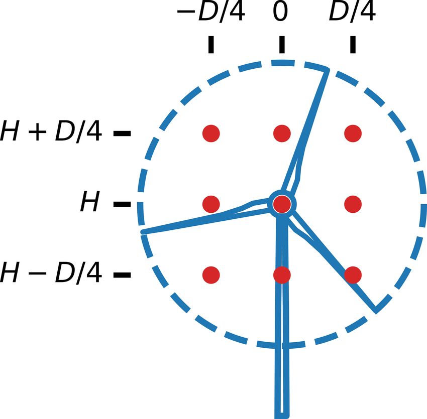
1150                                                                           A. P. J. Stanley et al.: Objective and algorithm

assumed after the best performance was within a tolerance         trades are done in a random order until a trade at each lo-
of 10−3 for 25 generations, or a maximum generation limit         cation has been evaluated. The three phases are repeated in
of 1000 was met. For the results in this paper, the maximum       order, search–trade–trade, until the objective function does
generation limit was never met. As the genetic algorithm was      not improve after a complete cycle of all three phases. The
used for both the gridded parameterization and the boundary-      repeated sweep algorithm is shown in Algorithm 3.
grid method, continuous variables were binary encoded with
8 bits each. This means that for the boundary-grid parame-        5.4   Gradient-based optimization
terization, the variables were encoded into 76 bits – 3 bits
for the integer number of rows, 3 bits for the integer number     The optimization algorithms discussed previously are
of columns, 6 bits for the integer number of turbines on the      gradient-free and can simultaneously optimize the number
boundary, and 8 bits for each of the 8 continuous variables.      of turbines and their layout in a wind power plant. Another
A rule of thumb for genetic algorithms is to use a popula-        way to optimize turbine number and layout in a wind power
tion size of 10 times the number of design variables (Martins     plant is with gradient-based optimization. Gradient-based al-
and Ning, 2020). For the gridded plant domain, we followed        gorithms cannot optimize integer design variables or discon-
this rule of thumb exactly because there was a large number       tinuous design spaces – both of which are conditions that ap-
of design variables. For the boundary-grid parameterization,      ply to the problem addressed in this paper. However, it is pos-
we used a population of 100, which was slightly less than         sible to repeat a gradient-based optimization multiple times
10 times the number of design variables. This gave us good        with different numbers of wind turbines and then choose the
results for our formulation. The genetic algorithm is repre-      overall best solution for the given objective. This process is
sented in Algorithm 2.                                            computationally expensive for two main reasons. First, a pri-
                                                                  ori, it is difficult to determine the approximate number of
5.3    Proposed method: repeated sweep algorithm
                                                                  turbines that will be optimal. This means it is necessary to
                                                                  repeat the optimization many times, using different numbers
The last optimizer we used was a novel repeated sweep al-         of wind turbines. Second, gradient-based optimizers are es-
gorithm. As far as we are aware, no method similar to our         pecially susceptible to converging to local minima in the de-
proposed repeated sweep algorithm has been used in past re-       sign space. This problem is also prevalent in gradient-free
search for wind power plant layout optimization. Like the         optimization but is more pronounced in gradient-based op-
greedy algorithm, this optimizer was only used with the grid-     timization. The problem can be mostly accounted for by re-
ded plant parameterization, where each of the design vari-        peating the optimization many times with different randomly
ables is an integer, either 0 or 1. The creation of this op-      initialized design variables, but this requires even more com-
timizer was inspired by attempting to apply gradient-based        putation.
optimization principles to discrete design variables. As de-         In this paper, our purpose was to compare some gradient-
scribed below, the algorithm works by comparing adjacent          free methods that could be effectively used to solve for the
points, and switching the values if it would improve the ob-      optimal turbine number and placement in a wind power plant.
jective function, which could be imagined as the discrete ver-    For one case discussed in Sect. 6.2 we also used gradient-
sion of a gradient. The repeated sweep algorithm consists of      based optimization in order to compare the results. For the
three phases. First is a single search phase, followed by two     optimizations in this section, the time required to evaluate
trade phases.                                                     the objective function was small, allowing us to quickly per-
   In the search phase, one by one and in a random order, the     form the hundreds of optimizations necessary to explore the
value at each potential turbine location is switched from 1       design space. To perform the gradient-based optimization,
to 0 or from 0 to 1. If the objective improves, the swapped       we swept through all of the possible numbers of wind tur-
value is kept; if not, the design variable retains its original   bines that could fit in the wind power plant without violating
value. This is done until every potential turbine location has    the spacing constraints, which was 2–18 turbines. For each
been evaluated, and the value has been changed or retained.       number of turbines, we performed 50 optimizations with ran-
In both trade phases, each potential turbine location is again    domly initialized turbine locations. This gave us relatively
searched through one by one. However, in these phases, in-        high confidence that the solution we found with the gradient-
stead of exploring adding or removing turbines (like in the       based optimization was near the global solution. We used
search phase), the potential turbine location trades values       finite-difference gradients for these optimizations, which do
with the cell adjacent to it. In the way we formulated the        not perform as well as analytic gradients, both in quality
problem, in the first trade phase, each position trades places    of the final solution and in computational expense. How-
with the cell to the right; in the second trade phase, each po-   ever, for the case in which we used the gradient-based op-
sition trades places with the cell above it. As with the search   timizer, the wind rose was simple and the number of design
phase, if a trade results in an improvement in the objective,     variables was relatively small, meaning the finite-difference
the trade is kept. If not, the trade is rejected and the origi-   gradients performed sufficiently well. For the results in this
nal locations are retained. Also, as with the search phase, the   paper, we used the open-source SLSQP (Sequential Least

Wind Energ. Sci., 6, 1143–1167, 2021                                                https://doi.org/10.5194/wes-6-1143-2021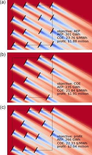
A. P. J. Stanley et al.: Objective and algorithm                                                                            1151

Squares Programming) optimizer available in SciPy (Virta-         full two-dimensional (2D) wind power plant layout optimiza-
nen et al., 2020; https://docs.scipy.org/doc/scipy/reference/     tions run for the different objectives and with the different
generated/scipy.optimize.minimize.html, last access: 30 Au-       optimization algorithms. The wind plants that we optimized
gust 2021).                                                       and discuss in this section are a small wind power plant with
                                                                  a unidirectional wind rose, a large wind power plant with a
5.5    Constraints                                                unidirectional wind rose, and a large wind power plant with
                                                                  a full wind rose. Finally in this section, we present results
In our layout optimizations, we assumed there were only two       from optimizing wind power plants for maximum profit with
constraints – a spacing constraint and a boundary constraint.     varying PPAs.
The turbines were constrained to be at least two rotor diam-
eters apart from each other. This minimum spacing is on the
small side and is used to exaggerate the differences in the       6.1   1D example
optimal solutions obtained with different objective function.     First we discuss a simple, 1D example to demonstrate the
The minimum spacing constraint implicitly defined the max-        effect different objective functions have on the optimal so-
imum number of turbines that could be placed in the wind          lution. For this example, we simulated a single row of wind
power plant. Additionally, turbines were constrained to re-       turbines in line with the wind, which had a constant speed
main inside a prescribed boundary.                                of 10 m s−1 . The length of this row was fixed at 25 km, and
                                                                  the turbines were equally spaced. For this scenario, we calcu-
6     Results                                                     lated the value of each objective as a function of the number
                                                                  of wind turbines in the simple wind power plant; results are
In this section, we discuss the results of our wind power plant   shown in Fig. 6.
simulations and optimizations. Included in this section is a         One key takeaway from this figure is that the optimal num-
simple, one-dimensional (1D) sweep of the different objec-        ber of turbines for each objective is very different. Obviously,
tive functions versus the number of wind turbines, and then       a wind plant designed for maximum AEP will look very

https://doi.org/10.5194/wes-6-1143-2021                                                Wind Energ. Sci., 6, 1143–1167, 2021
1152                                                                                    A. P. J. Stanley et al.: Objective and algorithm

Figure 6. Different objectives as a function of the number of turbines in the wind power plant. For this example, the turbines are in line with
the wind direction and are equally spaced in a wind power plant with a fixed length. From left to right, the objectives represented here are
annual energy production (AEP), cost of energy (COE), and annual profit.

different than wind plants designed with other objectives in              the increase in cost. It makes sense that the wind power plant
mind. When maximizing AEP, there is no penalty for the ex-                optimized for AEP has the most wind turbines, 23 in this ex-
tra costs associated with building extra turbines. As long as             ample, because more turbines are added until the wake effect
adding another turbine produces more energy, it is superior –             from adding an extra turbine outweighs the additional power
no matter how marginal the increase in energy and how large               it provides.

Wind Energ. Sci., 6, 1143–1167, 2021                                                          https://doi.org/10.5194/wes-6-1143-2021
A. P. J. Stanley et al.: Objective and algorithm                                                                             1153

   On the other hand, when COE is the objective, the optimal       straints. One must remember that these results were obtained
number of wind turbines is just nine, much lower than for the      from a very simple design space sweep with all wind turbines
AEP objective. If the cost of the wind plant was modeled as        exactly in line with the wind. Because real wind power plants
a linear function of the number of turbines, the optimal COE       are built in two dimensions, with full wind-direction vari-
solution would be just one turbine. A single turbine would         ability, it is actually possible to build turbines much closer
have no wake interference from other turbines and would,           together than is indicated in Fig. 6.
therefore, produce energy for the lowest cost. However, there         As demonstrated in Fig. 6, when determining the number
are some economies of scale involved with wind plant de-           of wind turbines to build in a wind power plant, an appro-
velopment, represented in our cost model by the decrease in        priate objective is essential to achieving a desirable solution.
BOS costs with increasing power capacity. This means there         This is true of any optimization problem, but it is particu-
is some optimum greater than one where the wake interfer-          larly important to remember for this application. COE is an
ence is still relatively low and the costs per turbine in the      extremely common objective function in wind plant design
wind plant are decreasing steeply with additional turbines.        – and rightfully so. However, as demonstrated in this simple
   Finally, a completely different solution is obtained when       example, the optimal number of turbines to minimize COE
optimizing the wind power plant for maximum profit. While          is suboptimal if the aim is to maximize annual profit, which
the COE objective optimizes the ratio between the value a          may (or may not) be what is most important to those design-
wind plant produces and the cost, the profit objective opti-       ing the wind power plant. In this specific example, the op-
mizes the difference between the value a wind plant produces       timal number of turbines for COE results in USD 5.1 mil-
and the cost. At first, it may seem nonintuitive that the solu-    lion of annual profit with a PPA of USD 50 MWh−1 , just
tion for optimal profit is different than the solution for opti-   72 % of the optimal profit of USD 7.1 million. This signif-
mal COE because minimized costs should be related to more          icant difference in the optimal performance and wind plant
profit. In Fig. 6, notice that the optimal COE solution is nine    design for different objectives has important implications for
turbines and produces a COE of about USD 23 MWh−1 . In             techno-economic considerations in wind plant design. Eco-
this case, energy generation and, therefore, revenue genera-       nomic factors drastically change the optimal solution, which
tion are limited because of the small number of turbines. For      highlights the importance of having accurate cost models and
18 wind turbines, a slightly higher COE is achieved of about       again identifying the correct objective for design and opti-
USD 25 MWh−1 . From a COE perspective, this is subopti-            mization.
mal. However, the additional revenue produced from the ex-            Historically, capacity expansion models have assumed a
tra turbines outweighs the increase in COE. The exact num-         constant power density that does not vary with the PPA.
ber of turbines for optimal profit depends on the monetary         Not only does Fig. 6 demonstrate the differences between a
value of the energy, which is defined with the PPA. This           minimum COE objective and a maximum profit objective,
means that the optimal solution is different depending on the      but it also shows that the cost modeling assumptions can
PPA, represented by the different colors in the subfigure on       greatly affect the optimal number of turbines in a given land-
the right. The optimal number of turbines increases from 13        constrained wind plant. Aggressive carbon reduction scenar-
to 16 as the PPA increases from USD 30 to USD 50 MWh−1 ,           ios or other renewable energy goals typically result in high
then again to 18 as the PPA increases to USD 70 MWh−1 .            PPAs for renewables, which would lead to a higher optimal
However, when the PPA increases to USD 90 MWh−1 , the              number of turbines and higher capacity densities for land-
optimal number of turbines remains at 18. This is because          constrained sites. This has important implications for capac-
the number of turbines is not continuous and is only repre-        ity expansion models and could play a role in the future de-
sented by integer values. For a given scenario, different PPA      ployment of wind, as capacity density may often be much
thresholds could be defined, above which the optimal num-          higher than is currently assumed.
ber of turbines would increase by one. From Fig. 6, it appears
that the optimal number of turbines is more sensitive at low
PPA values and becomes less sensitive as PPA increases.            6.2   Small plant with unidirectional wind rose
   As described previously, Fig. 6 shows different metrics as
a function of the number of turbines in a 1D wind power            With the 1D sweep of the design space complete to pro-
plant. In addition to the number of turbines shown on the bot-     vide some intuition about the different objective functions,
tom axis, this figure also shows the turbine spacing in rotor      we now discuss a simple layout optimization for a small wind
diameters on the top axis. While this axis is useful in un-        power plant with a unidirectional wind rose. As stated before,
derstanding the results from a more familiar perspective, one      we performed the optimization of each objective using a grid-
must be careful not to interpret these values incorrectly. The     ded domain, optimized with a greedy algorithm, a genetic al-
optimal turbine rotor diameter spacing reported in this fig-       gorithm, and a repeated sweep algorithm. We also optimized
ure is around 10 for AEP, 24 for COE, and between 12 and           a boundary-grid layout parameterization with a genetic algo-
18 for profit. These are very large turbine spacings for a wind    rithm. Also, as mentioned before, for this small wind plant,
plant and are likely infeasible because of land or cabling con-    we optimized the layouts using gradient-based optimization.

https://doi.org/10.5194/wes-6-1143-2021                                                 Wind Energ. Sci., 6, 1143–1167, 2021
1154                                                                           A. P. J. Stanley et al.: Objective and algorithm

   For this small wind power plant optimization, we assumed       6.2.1   Small power plant with unidirectional wind rose:
the domain was square with 800 m sides. The wind came                     different objectives
from a direction of 300◦ , or 30◦ north of west. The wind
speed was assumed constant at 10 m s−1 , which is close to        First, we will discuss the differences between the optimal so-
the rated wind speed for our turbine model. The PPA was           lutions for the different objective functions. For optimal AEP,
assumed to be USD 30 MWh−1 , which is close to the COE            the best solution has as many turbines as the optimizer can
solutions that were achieved, and is within the range of          fit into the wind power plant without violating spacing con-
the PPAs of real wind farms from the past few years (see          straints. As can be seen in the top subplot of Fig. 7, the op-
Fig. 16). For the gridded design variables, the domain was        timal layout has turbines that are spaced very close together.
discretized into a 10-by-10 grid. We ran each optimization        Wakes are strong in the flow field, which contains several tur-
method five times to convergence because the final solution       bines that are fully or partially waked. For this objective, it
is dependent on the randomly initialized population or design     does not matter if some turbines are greatly affected by wakes
space. Because each of the optimization algorithms has some       as long as their energy contribution is positive. Now, in this
stochastic qualities, with enough time and randomly initial-      case, the optimal solution had the maximum number of tur-
ized starts, each optimization method will potentially be able    bines as could fit into the boundary. However, from Fig. 6 we
to find a very good solution. However, we believe that five       see that even for the AEP objective, there is a point where
optimizations for each is enough to give a good idea of their     adding additional turbines actually becomes detrimental. We
performance relative to each other for each of the objective      also see from Fig. 6 that this could occur at a relatively large
functions.                                                        turbine spacing, between 9–10 rotor diameters. For the 1D
   Results for the small wind power plant optimizations with      sweep, the turbines are all exactly in line with the wind. Ad-
a unidirectional wind rose are shown in Table 2 and Fig. 7.       ditionally, rather than having two or three turbines waked in
Table 2 shows the optimization results and the computational      line, there are many in line with each other. This indicates
expense associated with each optimization method and for          that, in large part, the AEP is determined by deep array ef-
each objective function. The first column shows the objec-        fects. For the small wind plant layout optimization discussed
tive function, and the second column shows the optimiza-          in this section, there are at most three turbines in line with
tion method. The third column gives the optimized number          each other. In this case, adding turbines, even if they are fully
of turbines in the wind plant, the fourth column shows the        waked, increases the AEP. If we were to repeat the optimiza-
average turbine spacing in rotor diameters associated with        tion for a much larger domain we could potentially see re-
that number of turbines, the fifth column provides the best       sults similar to Fig. 6, where having too many turbines could
solution from the five optimizations. In this column, the best    actually be detrimental for AEP.
and worst solutions are indicated and bold in the table. The          While the wind power plant optimized for AEP maximizes
sixth column shows the best solution normalized by the best       the number of turbines in the design space, the wind plant op-
solution out of all of the optimization methods for the given     timized for minimum COE looks very different. This wind
objective. The seventh and eighth columns provide the to-         plant has 11 turbines, as opposed to 16 for maximum AEP.
tal time required to run the five optimizations, in seconds       The turbines are arranged such that waking is minimal. For
and hours, respectively. Finally, the ninth column shows total    this objective, it appears that the optimizer maximizes the
number of calls to the wind farm evaluation, or function calls,   number of unwaked wind turbines. For this case, we can con-
required to run the five optimizations for each optimization      clude that when the turbines are waked, the loss in energy
method. The separate, italicized bottom row for each objec-       production outweighs the benefits gained from economies of
tive in this table shows the gradient-based optimization re-      scale in the cost model. Therefore, additional turbines are
sults. Figure 7 shows the flow field for the best layout for      good if they meet some minimum power production require-
each objective function. These are the layouts corresponding      ment, which is dictated by the cost model.
to the indicated bold cells in Table 2. These flow fields show        For the last objective, profit with a PPA of
a horizontal slice of the wind power plant at the turbine hub     USD 30 MWh−1 , the optimized number of turbines is
height. The black lines represent the wind turbines, the red      13. This is between the optimal number of turbines for the
areas represent faster freestream wind speed, and the blue ar-    COE and AEP objectives. When optimizing for profit, the
eas represent a slower waked wind speed. We did not include       solution appears to be a balance between minimizing COE
a color legend because we only wish to demonstrate qualita-       and maximizing AEP. A turbine is allowed to be waked as
tive information with this figure; therefore, exact values are    long as the gains from the energy it produces outweigh the
not important for this purpose.                                   costs of adding the extra turbine. As will be discussed in
                                                                  more detail in Sect. 6.6, the point where adding an additional
                                                                  turbine is no longer profitable is determined by the PPA. A
                                                                  lower PPA will drive the solution for maximum profit toward
                                                                  the solution for minimum COE, while a higher PPA will
                                                                  drive it toward the solution for maximum AEP.

Wind Energ. Sci., 6, 1143–1167, 2021                                                 https://doi.org/10.5194/wes-6-1143-2021
A. P. J. Stanley et al.: Objective and algorithm 1155
Table 2. Complete optimization results for the small wind power plant with unidirectional wind rose. “BG” indicates the boundary-grid
design variables, and “GB” stands for the gradient-based optimization. The bold entries indicate the best and worst solutions for each
objective.
Objective Optimization No. turbines Avg spacing (D) Optimal value Normalized Time (s) Time (h) Function
optimal value calls
AEP (GWh) greedy grid 12 2.76 238 (worst) 0.792 15 0.004 2267
genetic grid 16 2.26 293 0.973 1867 0.52 105 872
sweep grid 15 2.36 270 0.897 4 0.001 204
genetic BG 16 2.26 301 (best) 1.000 1022 0.28 50 519
GB 17 2.17 299 0.993 12 082 3.36 651 265
COE (USD MWh−1 ) greedy grid 10 3.14 22.16 (worst) 1.015 11 0.003 1860
genetic grid 11 2.93 21.84 (best) 1.000 1443 0.40 106 755
sweep grid 10 3.14 21.88 1.002 8 0.002 656
genetic BG 9 3.40 22.16 1.014 319 0.09 26 604
GB 11 2.93 21.93 1.004 12 071 3.35 655 392
Annual profit (USD MM) greedy grid 11 2.93 1.88 0.918 15 0.004 2208
genetic grid 12 2.76 1.99 0.971 1306 0.36 95 687
sweep grid 12 2.76 1.76 (worst) 0.860 5 0.001 341
genetic BG 14 2.48 1.85 0.905 532 0.15 36 510
GB 13 2.61 2.04 (best) 1.000 13 130 3.65 702 650
We want to emphasize that the results we show are not
meant to demonstrate exact solutions or guidelines for deter-
mining the number of turbines in a wind power plant. Spe-
cific solutions will depend on wind resources, turbine param-
eters, boundary shape and size, PPA, constraints, and other
factors. Our purpose is to demonstrate that the optimal num-
ber of turbines and their layout are completely different de-
pending on the objective. The true objective must be care-
fully formulated when optimizing the layout of a wind power
plant. Figure 8 shows how the wind plants optimized for
the three different objectives compare in other metrics. We
demonstrated objectives of AEP, COE, and profit and how
they all produce different solutions. All of the wind plants
optimized for a specific metric greatly underperform in the
other metrics that we calculated. The one exception is the
optimal profit solution, which also accomplishes a relatively
low COE.
While we included three specific objective functions in
this paper, there are many other considerations that could
be included in the objective. For example, it may be desir-
able to maximize the profit generated by each turbine in the
wind power plant above some minimum value. This would
keep the optimizer from adding a turbine that only provided
a marginal return on investment. One could also optimize for
profit or COE while constraining the AEP to be above some
desired minimum value. When using mathematical optimiza-
Figure 7. The optimal layouts for each objective for the small wind tion, the objective function must be designed to truly repre-
power plant with a unidirectional wind rose. From top to bottom, sent the desired performance because this will drive the final
the associated objective functions are AEP, COE, and profit. The solution.
text within each figure provides the values for all three metrics for
each wind plant.
https://doi.org/10.5194/wes-6-1143-2021 Wind Energ. Sci., 6, 1143–1167, 20211156 A. P. J. Stanley et al.: Objective and algorithm
Figure 8. A comparison of the performance metrics of the three different wind power plants optimized for different objective functions.
These results are shown for the small wind plant with a unidirectional wind rose.
6.2.2 Small power plant with unidirectional wind rose: solution, within 0.2 % of the best solution. Like the greedy
different algorithms algorithm, the repeated sweep algorithm has a step that re-
lies on greedily placing turbines in the domain if they result
In this section, we discuss the performance of the solutions in an improvement of the objective function. This algorithm
found with each optimization strategy and their computa- has difficulty placing the turbines without violating spacing
tional expense. This information is presented in the last five constraints for objectives that have many turbines in the op-
columns of Table 2. As explained previously, the fifth col- timal solution. For the COE objective however, the optimal
umn shows the optimized solution, and the sixth shows the number of turbines was much fewer. Thus the repeated sweep
normalized value, to easily see how the optimized solutions algorithm could place the turbines and move them around to
compare to each other. The last three columns are measures a certain extent to find an excellent solution for this objec-
of the computational expense. The time columns are straight- tive. The negligible computational expense for this algorithm
forward and show the total wall time required to run the op- could justify its use for this scenario, for an objective with
timizations. For this paper, everything was run without par- optimal turbine spacings that are sufficiently larger than the
allelization on a laptop with a 2.4 GHz 8-core Intel proces- minimum spacing constraints.
sor. However, just the time as a measure of computational The genetic algorithm with the gridded plant domain per-
expense may be misleading. There is another overhead in formed very well for each objective function. It even out-
the optimization time other than just objective function calls; performed the gradient-based optimization for the COE ob-
therefore, we included a column for total objective function jective and performed within 3 % of the best solution found
calls and run time, which together give a decent representa- for the AEP and profit objectives. However, the computa-
tion of the total computational expense of each algorithm. tional expense was high, requiring the most time of any of
For this small wind power plant with the unidirectional the gradient-free algorithms and by far the most function
wind rose, the greedy algorithm did not perform very well. It calls. However, because this problem was relatively small,
found the worst solution for both the AEP and COE objec- the computational expense was not prohibitive.
tives and only the third best solution for the profit objective, The boundary-grid optimization solved with a genetic al-
but it still underperformed by more than 8 % compared to the gorithm performed in the middle of the pack for the gradient-
best solution in this objective. This algorithm relies on plac- free algorithms. It performed very well with the AEP ob-
ing turbines far apart to get the maximum benefit possible at jective but poorly with the COE and profit objectives. This
each step of the optimization. Because the domain for this was because of the small wind plant area. The boundary-grid
scenario was small, this made it difficult to add additional formulation forces turbines to be equally spaced around the
turbines without violating the spacing constraint. Doing so boundary. With a unidirectional wind rose, this means that
would require adjusting the location of multiple turbines at some turbines will always be in the back of the power plant
once to make room, which is not something this algorithm relative to the incoming wind. As discussed before, waked
does. Although the computational expense for the greedy al- turbines were very detrimental for COE and, by extension,
gorithm in this scenario was minimal, its poor performance detrimental from a profit perspective as well.
does not justify its use. Finally, the gradient-based optimizer, while sweeping
For the objectives with higher turbine density, AEP and across the number of wind turbines, performed well for each
profit, the repeated sweep algorithm performed poorly. The objective function. Because this algorithm uses continuous
answers for these objectives were either the worst or second design variables and allows full access to the wind plant do-
worst solution found. However, for the COE objective this main, permitting each turbine to be placed wherever the op-
algorithm performed quite well and found the second best timizer deems best, we always expected the gradient-based
Wind Energ. Sci., 6, 1143–1167, 2021 https://doi.org/10.5194/wes-6-1143-2021You can also read