Ocean dynamic equations with the real gravity - Nature
←
→
Page content transcription
If your browser does not render page correctly, please read the page content below
www.nature.com/scientificreports
OPEN Ocean dynamic equations
with the real gravity
Peter C. Chu
Two different treatments in ocean dynamics are found between the gravity and pressure gradient
force. Vertical component is 5–6 orders of magnitude larger than horizontal components for the
pressure gradient force in large-scale motion, and for the gravity in any scale motion. The horizontal
pressure gradient force is considered as a dominant force in oceanic motion from planetary to small
scales. However, the horizontal gravity is omitted in oceanography completely. A non-dimensional C
number (ratio between the horizontal gravity and the Coriolis force) is used to identify the importance
of horizontal gravity in the ocean dynamics. Unexpectedly large C number with the global mean
around 24 is obtained using the community datasets of the marine geoid height and ocean surface
currents. New large-scale ocean dynamic equations with the real gravity are presented such as
hydrostatic balance, geostrophic equilibrium, thermal wind, equipotential coordinate system, and
vorticity equation.
Gravity is greatly simplified in oceanography from a three-dimensional vector field [g = (gλ, gφ, gz)] with (λ, φ, z)
being the (longitude, latitude, height) and (i, j, k) being the corresponding unit vectors with eastward positive
for i, northward positive for j, and upward positive (in the Earth radial direction) for k to a vertical vector (−g0k)
with the uniform gravity g0 = 9.81 m/s2. The feasibility of such a practice has never been challenged because the
horizontal components (gλ, gφ) are much smaller (5–6 orders of magnitudes) than the vertical component gz
and the deviation of the magnitude of gz to g0 is also very small. However, similar situation also occurs with the
three-dimensional pressure gradient force: the horizontal pressure gradient force is much smaller (5–6 orders
of magnitudes) than the vertical pressure gradient force in large-scale oceanic motion. The horizontal pressure
gradient forces are considered important in oceanic motion for any scales. Thus, the feasibility to neglect the
horizontal gravity components (gλ, gφ) against the vertical gravity (gz) needs to be investigated. The correct
approach is to compare the horizontal gravity with the horizontal forces such as the Coriolis force or the hori-
zontal pressure gradient force.
Reference coordinate systems. The polar spherical coordinates (more popular) and oblate spherical
coordinates (less popular, see Appendix) are the reference coordinate system used in the Earth science. In all the
fields of the Earth science such as meteorology, oceanography, and geodesy, the horizontal component of any
vector A is on the spherical surface if the polar spherical coordinates are used or on the ellipsoidal surface if the
oblate spherical coordinates are used,
A = Ah + Az k, Ah = A i + Aϕ j (1)
no matter the variable is evaluated on the geoid, isobaric, isopycnal, or topographic-following surfaces. Ocean
numerical models have several representations of the vertical (i.e., the radial) coordinate such as z-coordinate1,2,
isopycnal coordinate3,4, topographic-following coordinate (i.e., sigma-coordinate)5,6. However, the horizontal
component of the vector A is always given by (1).
Three forms of the gravity. Three forms of gravity exist in geodesy and oceanography: the real gravity g(λ,
φ, z), the normal gravity [−g(φ)k], and the uniform gravity (−g0k, g0 = 9.81 m/s2). The real gravity (g) is a three-
dimensional vector field, which is decomposed into
g = gh + gz k, gh = g i + gϕ j (2)
where gh is the horizontal gravity component; and (gzk) is the vertical gravity component. The normal gravity
vector [−g(φ)k] (vertical vector) is associated with a mathematically modeled Earth (i.e., a rigid and geocentric
ellipsoid) called the normal Earth. The normal Earth is a spheroid (i.e., an ellipsoid of revolution), has the same
total mass and angular velocity as the Earth, and coincides its minor axis with the mean rotation of the E arth7.
Department of Oceanography, Naval Postgraduate School, Monterey, CA, USA. email: pcchu@nps.edu
Scientific Reports | (2021) 11:3235 | https://doi.org/10.1038/s41598-021-82882-1 1
Vol.:(0123456789)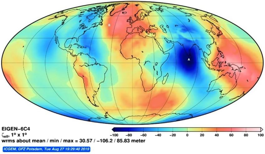
www.nature.com/scientificreports/
Similar to g(λ, φ, z), the normal gravity [−g(φ)k] is the sum of the gravitational and centrifugal accelerations
exerted on the water particle by the normal Earth. Its intensity g(φ) is called the normal gravity and determined
analytically. For example, the World Geodetic System 1984 uses the Somiglina equation to represent g(φ)8
1 + κ sin2 ϕ a2 − b2 bgp − age
g(ϕ) = ge
, e2 = ,κ = (3)
2
1 − e2 sin ϕ a2 age
where (a, b) are the equatorial and polar semi-axes; a is used for the Earth radius, R = a = 6.3781364 × 10⁶ m;
b = 6.3567523 × 10⁶ m; e is the spheroid’s eccentricity; ge = 9.780 m/s2, is the gravity at the equator; and gp = 9.832 m/
s2 is the gravity at the poles. The uniform gravity (−g0k) is commonly used in oceanography.
Real and normal gravity potential. Let (P, Q) be the Newtonian gravitational potential of the (real Earth,
normal Earth) and PR (= �2 r 2 cos2 ϕ/2)) be the potential of the Earth’s rotation. Let V = P + PR be the gravity
potential of the real Earth (associated with real gravity g) and E = Q + PR be the gravity potential of the normal
Earth [associated with the normal gravity -g(φ)k]. The potential of the normal gravity [−g(φ)k] is given by
E(ϕ, z) = −g(ϕ)z (4)
The gravity disturbance is the difference between the real gravity g(λ, φ, z) and the normal gravity [−g(φ)k]
oint9. The potential of the gravity disturbance (called the disturbing gravity potential) is given by
at the same p
T = V − E = P − Q. (5)
Consequently, the centrifugal effect disappears and the disturbing gravity potential (T) can be considered
a harmonic function. With the disturbing gravity potential T, the real gravity g (= gh + gzk) is represented by
∂T
gh = ∇h T, gz = −g(ϕ) + (6)
∂z
where ∇h is the horizontal vector differential operator. The geoid height relative to the normal Earth (i.e., refer-
ence spheroid) is given by Bruns’ formula10
T( , ϕ, 0)
N( , ϕ) = (7)
g0
Equations (5), (6), (7) clearly show that the fluctuation of the marine geoid is independent of the Earth rota-
tion and dependent on the disturbing gravity potential (T) evaluated at z = 0 only.
The disturbing static gravity potential (T) outside the Earth masses in the spherical coordinates with the
spherical expansion is given b y11
∞ l
l
GM R
T(r, , ϕ) = el
Cl,m − Cl,m cos m + Sl,m sin m Pl,m (sin ϕ), (8)
r r
l=2 m=0
where G = 6.674 × 10⁻¹¹m3kg−1 s−2, is the gravitational constant; M = 5.9736 × 1024 kg, is the mass of the Earth; r
is the radial distance with z = r−R; Pl,m (sin ϕ) are the Legendre associated functions with (l, m) the degree and
order of the harmonic expansion; (Cl,m , Cl,mel , S ) are the harmonic geopotential coefficients (Stokes parameters
l,m
with Cl,m belonging to the reference ellipsoid.
el
From Eqs. (4) and (5) the potential of the real gravity is given by
V = T − g(ϕ)z. (9)
From Eq. (6) the real gravity is represented by
∂T
g( , ϕ, z) = ∇h T + − g(ϕ) k (10)
∂z
The horizontal gravity component at the reference ellipsoid surface (z = 0) is obtained using (7) and (10)12,13
gh ( , ϕ, 0) = ∇h T = g0 ∇h N (11)
An approximate 3D gravity field for oceanography. According to Eq. (8) (i.e., the spectral of the
disturbing static gravity potential T), the ratio between T(λ, φ, z) to T(λ, φ, 0) through the water column can be
roughly estimated by
T( , ϕ, z) R
T( , ϕ, 0) ≈ (R + z) ≈ 1, 0 ≥ z ≥ −H( , ϕ)
(12)
where H is the water depth. Since R is the radius of the Earth and more than 3 orders of magnitude larger than
the water depth H. This leads to the first approximation that the surface disturbing gravity potential T(λ, φ, 0)
is used for the whole water column,
Scientific Reports | (2021) 11:3235 | https://doi.org/10.1038/s41598-021-82882-1 2
Vol:.(1234567890)
www.nature.com/scientificreports/
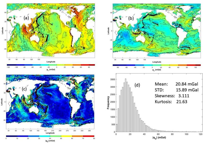
Figure 1. Digital data for EIGEN-6C4 geoid undulation (N) with 1° × 1°, computed online at the website http://
icgem.gfz-potsdam.de/home.
T( , ϕ, z) ≈ T( , ϕ, 0), 0 ≥ z ≥ −H( , ϕ) (13)
Since the deviation of the vertical component of the gravity (gz) to a constant (−g0) is 3–4 orders of magnitude
smaller than g0, it leads to the second approximation
gz ≈ −g0 (14)
With the two approximations, the near real gravity in the water column is given by
∂N ∂N
gx ( , ϕ, z) ≈ g0 , gy ( , ϕ, z) ≈ g0 , gz ( , ϕ, z) ≈ −g0 (15)
∂x ∂y
Correspondingly, the potential of the real gravity is approximately given by
V ( , ϕ, z) ≈ g0 [N( , ϕ) − z] (16)
where Eq. (9) is used.
Unexpectedly large horizontal gravity component. For simplicity, the local coordinates (x, y, z) are
used from now on to replace the polar spherical coordinates with x representing longitude (eastward positive)
and y representing latitude (northward positive). The local and spherical coordinate systems are connected by
∂ 1 ∂ ∂ 1 ∂ ∂ ∂
= , = , = (17)
∂x R cos ϕ ∂ ∂y R ∂ϕ ∂z ∂r
The EIGEN-6C4 m odel14,15, listed on the website http://icgem.gfz-potsdam.de/home, was developed jointly
by the GFZ Potsdam and GRGS Toulouse up to degree and order 2190 to produce global static geoid height
(N) dataset. Following the instruction, the author ran the EIGEN-6C4 model in 1° × 1° resolution for 17 s to
get the global N (Fig. 1) with mean value of 30.57 m, minimum value of -106.20 m, and maximum of 85.83 m.
Two locations on the marine geoid are identified with NA = − 99.76 m at A (80° W, 3° N) in the Indian Ocean,
and NB = 65.38 m at B (26° W, 45° N) in the North Atlantic Ocean, i.e., |ΔN|AB = 165.14 m. The big circle distance
between A and B is about ΔL = 7920 km. Equation (11) shows that the corresponding |gh| at z = 0 is computed by
| N|AB 165.14 m
= 9.81 m/s2 × (18)
gh
AB
= g0 = 20.45 mGal
L 7.920 × 10⁶ m
With the geoid height data obtained from the EIGEN-6C4, N(x, y), the horizontal gravity components gx (Fig. 2a)
and gy (Fig. 2b) at z = 0 are computed using Eq. (11). The magnitude of the horizontal gravity vector is calculated
by
2
2
(19)
gh (x, y) = gx (x, y) + gy (x, y) ,
Scientific Reports | (2021) 11:3235 | https://doi.org/10.1038/s41598-021-82882-1 3
Vol.:(0123456789)www.nature.com/scientificreports/
Figure 2. Horizontal gravity components (unit: mGal) at z = 0: (a) longitudinal component
(gλ), (b) latitudinal
component (gφ), (c) magnitude of the horizontal gravity vector gh , and (d) histogram of gh (from the
reference16). The source codes for the plots were written by the author ‘s research group using the Matlab
Version R2019b (https://www.mathworks.com/products/matlab.html).
as shown in Fig. 2c. The histogram of |gh| (Fig. 2d) indicates a positively skewed distribution with a long tail
extending to values larger than 100 mGal (1 mGal = 10−5 m s−2). The statistical characteristics of |gh| are 20.84
mGal as the mean, 15.89 mGal as the standard deviation, 3.11 as the skewness, and 21.63 as the kurtosis. The
statistical estimate of the mean intensity of the horizontal gravity |gh| (20.84 mGal) is coherent with the simple
calculation of |gh|AB between points A and B (20.45 mGal). The two values (20.84 mGal, 20.45 mGal) are unex-
pectedly large.
C number to identify importance of the horizontal gravity. The importance of the horizontal grav-
ity can be identified by a non-dimensional C number16 from the analysis of horizontal gravity versus the Coriolis
force,
gh
C(x, y, z) = (20)
f U
where f = 2Ωsinφ, is the Coriolis parameter; and U is the speed of the horizontal current. With Eq. (11) the C
number at z = 0 is given by
g0 |�N|
C0 (x, y) ≡ C(x, y, 0) = (21)
f U�L
where ΔL is the horizontal scale of the motion.
The Ocean Surface Current Analysis Real-time (OSCAR) third degree resolution 5-day mean surface cur-
rent vectors17 on 26 February 2020 (Fig. 3a) was downloaded from the website https://podaac-tools.jpl.nasa.
gov/drive/files/allData/oscar/ and the data at the same 1° × 1° grid points as the EIGEN-6C4 data were used.
The data represent vertically averaged surface currents over the top 30 m of the upper ocean, which consist of
a geostrophic component with a thermal wind adjustment using satellite sea surface height, and temperature
and a wind-driven ageostrophic component using satellite surface winds. The histogram of the OSCAR current
Scientific Reports | (2021) 11:3235 | https://doi.org/10.1038/s41598-021-82882-1 4
Vol:.(1234567890)www.nature.com/scientificreports/
Figure 3. (a) The world ocean surface current vectors on 26 February 2020 from the ocean surface current
analysis real-time (OSCAR) dataset which was downloaded from the website https://podaac-tools.jpl.nasa.gov/
/allData/oscar/, (b) histogram of the current speed U, and (c) histogram of the intensity of the Coriolis
drive/ files
force f U . The source codes for the plots were written by the author’s research group using the Matlab Version
R2019b (https://www.mathworks.com/products/matlab.html).
speed U(x, y) (Fig. 3b) indicates a positively skewed distribution with a long tail extending to values larger than
0.4 m/s. The statistical characteristics of U are 0.1397 m/s as the mean, 0.1414 m/s as the standard deviation,
3.013 as the skewness, and 21.01 as the kurtosis. The histogram of the corresponding Coriolis force |f |U(x, y)
(Fig. 3c) also shows a positively skewed distribution with a long tail extending to values larger than 2.5 mGal.
The statistical characteristics of |f |U are 0.8815 mGal as the mean, 1.029 mGal as the standard deviation, 3.379
as the skewness, and 20.24 as the kurtosis. Comparison between Figs. 2d and 3c leads to the fact that the mean
intensity of horizontal gravity component |gh | (= 20.84 mGal) is nearly 24 times as large as the mean intensity
of the Coriolis force identified from the OSCAR surface currents on 26 February 2020. Such unexpectedly large
horizontal gravity component is also shown in the world ocean distribution of (1/C0) values (Fig. 4a). The histo-
gram of (1/C0) (Fig. 4b) indicates a positively skewed distribution with a long tail extending to values larger than
0.18. The statistical characteristics of (1/C0) are 0.04238 as the mean, 0.04108 as the standard deviation, 1.447
Scientific Reports | (2021) 11:3235 | https://doi.org/10.1038/s41598-021-82882-1 5
Vol.:(0123456789)www.nature.com/scientificreports/
Figure 4. (a) The world ocean surface (z = 0) distribution of (1/C), and (b) histogram of (1/C). The source codes
for the plots were written by the author ‘s research group using the Matlab Version R2019b (https://www.mathw
orks.com/products/matlab.html).
as the skewness, and 4.481 as the kurtosis. Thus, the global mean of C0 is about 23.6, which is coherent with the
rough estimate given above using the geoid height data at the two points A and B (near 24).
New equations with the real gravity. Application of the Newton’s second law of motion into the ocean
for the large-scale motions with the Boussinesq approximation leads to
DU
ρ0 + 2 × U = −∇p + ρ∇V + ρ0 F (22)
Dt
if the pressure gradient force, gravitation, and friction are the only real forces. Here, = � j cos ϕ + k sin ϕ ,
is the Earth rotation vector with Ω = 2π/(86,400 s) the Earth rotation rate; ρ is the density; ρ0 = 1028 kg/m3, is the
characteristic density; U = (u, v), is the horizontal velocity vector; ∇ is the three dimensional vector differential
operator; and D/Dt is the total time rate of change; F = (Fx, Fy), is the frictional force and usually represented
using vertical eddy viscosity K,
∂ ∂u ∂ ∂v
Fx = K , Fy = K (23)
∂z ∂z ∂z ∂z
The continuity equation is given by
∂w
∇h · U + =0 (24)
∂z
where w is the vertical velocity. Substitution of (16) into (22) leads to
DU
ρ0 + 2 × U = −∇p + ρg0 ∇h N − g0 k + ρ0 F (25)
Dt
Scientific Reports | (2021) 11:3235 | https://doi.org/10.1038/s41598-021-82882-1 6
Vol:.(1234567890)www.nature.com/scientificreports/
Equation (25) can be easily used by any ocean numerical model with just adding the horizontal gravity
component represented by (ρg0 ∇h N).
Hydrostatic balance. Large-scale oceanic motion is hydrostatically balanced,
∂p ∂V
− +ρ = 0 ⇒ dp = ρdV (26)
∂z ∂z
Vertical integration of this equation from the marine geoid (i.e., V = 0) to any equipotential surface V leads
to the integral form of the hydrostatic balance
0
p= ρd Ṽ + ρ0 g0 (S − N) (27)
−V (x,y,z)
where S is the sea surface height; and the marine geoid surface (N) is the coincidence of the equipotential and
isobaric surfaces (i.e., balance of the 3D pressure gradient force and gravity on N).
Equipotential (‑V) coordinate system. The hydrostatic Eq. (27) clearly shows that a single valued mono-
tonic relationship exists between gravitational potential and the depth in each vertical water column. Thus, we
may use (-V) as the independent vertical coordinate. The negative sign is due to the vertical component of the
gravity is defined positive downward. The total derivative is expanded as
D ∂ Dx ∂ Dy ∂ D(−V ) ∂
= + + +
Dt ∂t Dt ∂x Dt ∂y Dt ∂(−V )
(28)
∂ ∂ ∂ ∂
= +u +v +ω
∂t ∂x ∂y ∂V
The continuity Eq. (24) becomes
∂ω
∇h · U + =0 (29)
∂V
here,
dV ∂V
ω≡ = U · ∇h V + w (30)
dt ∂z
where ω is the “vertical velocity” in the V-coordinate. Note that V is the static gravitational potential such that
∂V/∂t = 0.
Dynamic equations in the equipotential coordinate system. The horizontal pressure gradients can
be computed from (27),
0
∂p ∂V ∂ρ ∂(S − N)
=ρ + d Ṽ + ρ0 g0 ,
∂x ∂x ∂x ∂x
−V
(31)
0
∂p ∂V ∂ρ ∂(S − N)
=ρ + d Ṽ + ρ0 g0
∂y ∂y ∂y ∂y
−V
Substitution of (31) into (22) leads to the horizontal momentum equations
0
Du 1 ∂ρ ∂(S − N)
− fv = − d Ṽ − g0 + Fx (32a)
Dt ρ0 ∂x ∂x
−V
0
Dv 1 ∂ρ ∂(S − N)
+ fu = − d Ṽ − g0 + Fy (32b)
Dt ρ0 ∂y ∂y
−V
Extended geostrophic equilibrium and thermal wind relation. For steady state (no total derivative)
without friction, Eqs. (32a) and (32b) become the extended equations for the geostrophic currents
0
1 ∂ρ ∂(S − N)
−fvG = − d Ṽ − g0 (33a)
ρ0 ∂x ∂x
−V
Scientific Reports | (2021) 11:3235 | https://doi.org/10.1038/s41598-021-82882-1 7
Vol.:(0123456789)www.nature.com/scientificreports/
0
1 ∂ρ ∂(S − N)
fuG = − d Ṽ − g0 (33b)
ρ0 ∂y ∂y
−V
Vertical derivative of (33a) and (33b) leads to the extended thermal wind relation
0
∂vG g0 ∂ρ 1 ∂ 2ρ
−f = − d Ṽ (34a)
∂z ρ0 ∂x ρ0 ∂x∂z
−V
0
∂uG g0 ∂ρ 1 ∂ 2ρ
f = − d Ṽ (34b)
∂z ρ0 ∂y ρ0 ∂y∂z
−V
where the vertical differentiation of lower limit (-V) of the integrals of the righthand side of (33a) and (33b)
∂V
= gz ≈ −g0 (35)
∂z
is used.
Vorticity equation. Subtraction of the differentiation of the longitudinal component of Eq. (25) with
respect to y from the differentiation of the latitudinal component of Eq. (25) with respect to x leads to the vor-
ticity equation,
∂ζ ∂ζ ∂U
= −U · ∇h ζ − ω + βv − (ζ + f )∇h · U + k · × ∇h ω
∂t ∂V ∂V
(36)
g0 ∂Fy ∂Fx
+ J(ρ, N) + −
ρ0 ∂x ∂y
where J(ρ, N) = (∂ρ/∂x)(∂N/∂y) − (∂ρ/∂y)(∂N/∂x), is the Jacobian; β = df /dy is the latitudinal change of
the Coriolis parameter; and ζ = ∂v/∂x − ∂u/∂y is the vertical vorticity.
Conclusion
The non-dimensional C number is used to identify relative importance of the horizontal gravity and the Coriolis
force using the geoid height data (N) provided by the EIGEN-6C4 gravity model, and the Ocean Surface Current
Analysis Real-time (OSCAR) surface current vectors on 26 February 2020. Unexpectedly large value of the C
number (global mean around 24) may surprise both oceanographic and geodetic communities. It is very hard for
my oceanographic colleagues to accept such strong horizontal gravity (at z = 0), which is an order of magnitude
lager that the Coriolis force. Thus, in situ measurement of gravity may be needed for oceanography in addition
to the routine hydrographic and current meter measurements.
A geodesist may also be surprised that the horizontal gravity (z = 0) associated with the geoid height (N)
varying between -106.20 m to 85.83 m (well accepted by the geodetic community), which was produced by
a community gravity model (EIGEN-64C), generates the ocean currents with the intensity nearly 24 times as
large as the currents identified from the ocean surface current analysis real-time (OSCAR) (oceanographic
community product).
How to resolve such incoherency between the two communities on this issue becomes urgent. The new
ocean dynamic equations including the horizontal gravity may provide a theoretical framework to resolve the
incoherency since the potential of the real gravity (V) obtained from a geodetic gravity model is explicitly in
the dynamical equations. Besides, use of the real gravity in the ocean dynamics may ultimately resolve some
fundamental problems in oceanography such as reference level, and absolute geostrophic current calculation.
A new dynamic system for large-scale oceanic motion with the real gravity is presented such as hydrostatic
balance, geostrophic equilibrium, thermal wind, equipotential coordinate system, and the vorticity equation.
Close collaboration between the oceanographic and geodetic communities helps the use of the real gravity in
oceanography and the verification of the gravity model in geodesy with oceanographic data.
Appendix: Oblate spheroid coordinates versus polar spherical coordinates
This paper uses the polar spherical coordinates rather than the oblate spheroid coordinates for computational
simplicity with a small error (0.17%)18. The oblate spheroid coordinates share the same longitude (λ) but different
latitude (φob) and radial coordinate (representing vertical) (rob). The relationship between the oblate spheroid
coordinates (λ, φob, rob) and the polar spherical coordinates (λ, φ, r) is given b
y18
1 1
r 2 = rob
2
+ d 2 − d 2 sin2 ϕob , r 2 cos2 ϕ = (rob
2
+ d 2 ) cos2 ϕob (37)
2 2
where d is the half distance between the two foci of the ellipsoid. For the normal Earth, d = 521.854 km. The
vector differential operator in the oblate spheroid coordinates is represented by
Scientific Reports | (2021) 11:3235 | https://doi.org/10.1038/s41598-021-82882-1 8
Vol:.(1234567890)www.nature.com/scientificreports/
1 ∂ 1 ∂ 1 ∂
∇=i + j ob + k ob , z =r−R (38)
hob
∂ hϕ ∂ϕ hr ∂z
where R = 6.3781364 × 10⁶ m, is the semi-major axis of the normal Earth (Earth radius). The coefficients (hob
,
ϕ , hr ) are given by
hob ob
r r 2 − 12 d 2 + d 2 sin2 ϕ
1 1
hob
= r 2 + d 2 cos ϕ, hob
ϕ = r 2 − d 2 + d 2 sin2 ϕ, hob
r =
. (39)
2 2 r 4 − 41 d 4
However, the vector differential operator in the polar spherical coordinates is represented by
1 ∂ 1 ∂ ∂
∇=i +j +k . (40)
r cos ϕ ∂ r ∂ϕ ∂z
Received: 7 September 2020; Accepted: 4 January 2021
References
1. Sun, F., Kim, V. S., Huang, B. & Wang, D. Water exchange between the subpolar and subtropical North Pacific Ocean in an OGCM.
Sci. China D 47, 37–48 (2004).
2. Chu, P. C., Fan, C. W. & Cai, W. J. P vector method evaluated using modular ocean model (MOM). J. Oceanogr. 54, 185–198 (1998).
3. Wang, D., Wang, J. & Wu, L. Regime shifts in the North Pacific simulated by a COADS-driven isopycnal model. Adv. Atmosph.
Sci. 20, 743–754 (2003).
4. Chu, P. C. & Li, R. F. South China Sea isopycnal surface circulations. J. Phys. Oceanogr. 30, 2419–2438 (2000).
5. Chu, P. C. & Fan, C. W. Sixth-order difference scheme for sigma coordinate ocean models. J. Phys. Oceanogr. 27, 2064–2071 (1997).
6. Chu, P. C., Lu, S. H. & Chen, Y. C. Evaluation of the Princeton Ocean model using the South China Sea Monsoon experiment
(SCSMEX) data. J. Atmos. Oceanic Technol. 18, 1521–1539 (2001).
7. Vaniček, P. & Krakiwsky, E. Geodesy: The Concepts 697 (North-Holland, Amsterdam, 1986).
8. National Geospatial-Intelligence Agency. Department of Defense World Geodetic System 1984 (WGS84). Its definition and relation-
ships with local geodetic systems. NIMA TR8350.2., 3rd Edition, Equation 4–1 (1984).
9. Hackney, R. I. & Featherstone, W. E. Geodetic versus geophysical perspectives of the ‘gravity anomaly’. Geophys. J. Int. 154, 35–43
(2003).
10. Sandwell, D. T. & Smith, W. H. F. Marine gravity anomaly from Geosat and ERS 1 satellite altimetry. J. Geophys. Res. 102(B5),
10039–10054 (1997).
11. Kostelecký, J., Klokočnìk, J., Bucha, B., Bezdĕk, A. & Fӧrste, C. Evaluation of the gravity model EIGEN-6C4 in comparison
with EGM2008 by means of various functions of the gravity potential and by BNSS/levelling. Geoinform. FCE CTU. https://doi.
org/10.14311/gi.14.1.1 (2015).
12. Chu, P. C. Two types of absolute dynamic ocean topography. Ocean Sci. 14, 947–957 (2018).
13. Chu, P. C. A. Complete formula of ocean surface absolute geostrophic current. Nat. Sci. Rep, 10, Article number 1445 (2020).
14. Ince, E. S. et al. ICGEM: 15 years of successful collection and distribution of global gravitational models, associated services, and
future plans. Earth Syst. Sci. Data 11, 647–674 (2019).
15. Förste, C., Bruinsma, S.L., Abrikosov, O., Lemoine, J.M., Marty, J.C., Flechtner, F., Balmino, G., Barthelmes, F., & Biancale, R.
EIGEN-6C4. The latest combined global gravity field model including GOCE data up to degree and order 2190 of GFZ Potsdam
and GRGS Toulouse, https://doi.org/10.5880/icgem.2015.1 (2014).
16. Chu, P. C.Occurrence of spurious geostrophic currents on the marine geoid without horizontal gravity component. Nat. Sci. Rep, in
press (2020).
17. ESR. OSCAR third deg. ver. 1. PO.DAAC, CA, USA. Dataset accessed [2020-11-10] athttps://doi.org/10.5067/OSCAR-03D01
(2009).
18. Gill, A. E. Atmosphere-Ocean Dynamics. International Geophysics Series Vol. 30, 91–94 (Academic Press, New York, 1982).
Acknowledgements
The author thanks the International Centre for Global Erath Models (ICGEM) for the EIGEN-6C4 geoid undu-
lation data, and the NASA Jet Propulsion Laboratory for the OSCAR Third Degree Resolution Ocean Surface
Currents. He also thanks Mr. Chenwu Fan for computational assistance, and the Naval Postgraduate School
Research Office for paying the publication cost.
Author contributions
P.C.C. designed the project, obtained the datasets, conducted the computation, and wrote the manuscript.
Competing interests
The author declares no competing interests.
Additional information
Correspondence and requests for materials should be addressed to P.C.C.
Reprints and permissions information is available at www.nature.com/reprints.
Publisher’s note Springer Nature remains neutral with regard to jurisdictional claims in published maps and
institutional affiliations.
Scientific Reports | (2021) 11:3235 | https://doi.org/10.1038/s41598-021-82882-1 9
Vol.:(0123456789)www.nature.com/scientificreports/
Open Access This article is licensed under a Creative Commons Attribution 4.0 International
License, which permits use, sharing, adaptation, distribution and reproduction in any medium or
format, as long as you give appropriate credit to the original author(s) and the source, provide a link to the
Creative Commons licence, and indicate if changes were made. The images or other third party material in this
article are included in the article’s Creative Commons licence, unless indicated otherwise in a credit line to the
material. If material is not included in the article’s Creative Commons licence and your intended use is not
permitted by statutory regulation or exceeds the permitted use, you will need to obtain permission directly from
the copyright holder. To view a copy of this licence, visit http://creativecommons.org/licenses/by/4.0/.
© The Author(s) 2021
Scientific Reports | (2021) 11:3235 | https://doi.org/10.1038/s41598-021-82882-1 10
Vol:.(1234567890)You can also read