Optimization and Stability of Heat Engines: The Role of Entropy Evolution - MDPI
←
→
Page content transcription
If your browser does not render page correctly, please read the page content below
entropy
Article
Optimization and Stability of Heat Engines: The Role
of Entropy Evolution
Julian Gonzalez-Ayala 1,2, * , Moises Santillán 3 , Maria Jesus Santos 1,2 , Antonio Calvo
Hernández 1,2 and José Miguel Mateos Roco 1,2
 1   Departamento de Física Aplicada, Universidad de Salamanca, 37008 Salamanca, Spain;
     smjesus@usal.es (M.J.S.); anca@usal.es (A.C.H.); roco@usal.es (J.M.M.R.)
 2   Instituto de Física Fundamental y Matemáticas, Universidad de Salamanca, 37008 Salamanca, Spain
 3   Centro de Investigación y Estudios Avanzados del IPN Unidad Monterrey, Apodaca, NL 66600, Mexico;
     msantillan@cinvestav.mx
 *   Correspondence: jgonzalezayala@usal.es

 Received: 23 October 2018; Accepted: 7 November 2018; Published: 9 November 2018

 Abstract: Local stability of maximum power and maximum compromise (Omega) operation regimes
 dynamic evolution for a low-dissipation heat engine is analyzed. The thermodynamic behavior of
 trajectories to the stationary state, after perturbing the operation regime, display a trade-off between
 stability, entropy production, efficiency and power output. This allows considering stability and
 optimization as connected pieces of a single phenomenon. Trajectories inside the basin of attraction
 display the smallest entropy drops. Additionally, it was found that time constraints, related with
 irreversible and endoreversible behaviors, influence the thermodynamic evolution of relaxation
 trajectories. The behavior of the evolution in terms of the symmetries of the model and the applied
 thermal gradients was analyzed.

 Keywords: heat engine; local stability; maximum power regime; maximum Omega regime; entropy
 production

1. Introduction
      The relevance of heat devices optimization and the searching for global properties of energy
converters is increasing due to a growing need of energetic requirements; not only for a better
use of available energy, but also for maintenance cost, operation life-time, scale related control
issues, etc. All these problems involve entropy production (∆S),  ˙ heat waste, power output (P) and
efficiency η [1,2]. Along with maximum power and maximum efficiency or minimum entropy
production, compromise based figures of merit have been found very valuable in the optimization
analysis of heat devices [3–19]. In this framework, the so-called Ω function, defined as Ω ≡ Pgain − Ploss ,
was proposed, offering useful insights since it represents a trade off between maximum power gain
(Pgain ≡ P − Pmin ) and minimum power loss (Ploss ≡ Pmax − P), with respect to the minimum and
maximum available power output for a heat engine. Besides, it is easy to implement in any energy
converter, isothermal or non-isothermal, because it does not require the explicit evaluation of the
entropy generation, and it is independent on environmental parameters.
      Recently, it has been pointed out that the problem of local stability of operation regimes can be
related with the regime’s optimization itself [20,21]. Thus, the effects of external perturbations on
the operation regime and on the energetic properties such as power output, efficiency and entropy
production, can be addressed. A natural question arises: Could entropy give us information to
distinguish particular behaviors inside the operation regimes’ basin of attraction? Recent papers have
explored this question using a somewhat simple model, the so-called low-dissipation heat engine

Entropy 2018, 20, 865; doi:10.3390/e20110865                                  www.mdpi.com/journal/entropy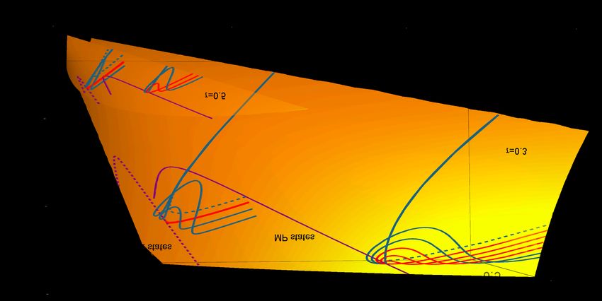
Entropy 2018, 20, 865                                                                                    2 of 12

(LD-HE), which departs from a first order approximation in the entropy generation of irreversible
heat devices [5,22–24]. Despite its simplicity, this model can be related with more complex heat
engines’ models [6,25–34]. These studies do not consider any specific information on the nature of
the heat conduction mechanism but focus, instead, on dissipation and operation time symmetries,
along with temporal constraints. Thus, due to its broad generality and independence of any heat
transfer law, the low-dissipation approximation could be useful to provide general thermal properties
for a variety of heat devices models in connection with its stability.
      Among the mentioned connections of the low dissipation model, several scales are involved,
from macroscopic models to microscopic ones. However, few systems have been analytically
solved and limited precision in the control variables remains as an open question, being this the
rationale for this stability study. In fact, in [35], it has been pointed out the lack of a systematic and
quantitative description of how limited control affects the performance of heat engines. This problem
is closely connected with some recent works regarding power fluctuations and large efficiencies
(see, for example, [35–37]). In a related line of thought to this work, Pietzonka and Seifert proposed
constancy as an additional ingredient in optimization [36].
      Since the specific mechanisms that cause heat flows in LD-HE’s models are unknown, for the
study of local stability, we introduce ad hoc restitutive forces to perform such stability analysis.
In fact, different restitutive forces are associated with different system’s dynamics and stable points
characteristics, as discussed in References [20,21]. This work focuses on the simplest case of restitutive
forces, linearly dependent on deviations from the stationary state in power output and output heat
flux released to the cold heat reservoir. Such forces yield a rich dynamics of the basin of attraction in
terms of the symmetries and the external bath temperatures. Consequently, a relevant behavior on the
entropy trajectories is observed in connection with the two optimized operation performance regimes.
      The work is organized as follows. For self contained purposes, Section 2 summarizes some
previous relevant results related with the LD-HE and the maximum power (MP) and maximum
Omega (MΩ) operation regimes. In Section 3, the stability dynamics and the main characteristics of the
basin of attraction in relation with irreversible and endoreversible behaviors are analyzed. In Section 4,
a comparison of the evolution behavior of entropy production, power output and efficiency when
the system evolves toward: (a) the stable point; or (b) the nullcline and eventually diverging to a
nonphysical, no-heat engine state. Finally, some concluding remarks are presented in Section 5.

2. Low Dissipation Model and Maximum Power and Omega Regimes
      The low-dissipation approximation considers a first order irreversible depart from a Carnot cycle.
The dissipation occurs in the contact with thermal reservoirs. As usual, the adiabatic processes are
consider as instantaneous. Accordingly, the exchanged heat with the cold (at temperatureTc ) and hot
(at temperature Th > Tc ) thermal reservoirs are modeled as [5]:

                                                         Σ

                                       Qh   = Th ∆S 1 − h      ,                                            (1)
                                                       ∆Sth
                                                           Σc

                                       Qc   = Tc ∆S −1 −         ,                                          (2)
                                                         ∆Stc

where tc , th are, respectively, the contact times with the hot and cold reservoirs. ∆S is the entropy
change of the baseline Carnot cycle along the hot isothermal process; and Σc , Σh are the dissipation
coefficients, containing all the information regarding intrinsic dissipation properties.
     By defining the dimensionless variables Σ  e c ≡ Σc /(Σc + Σh ), α ≡ tc /(tc + th ) and et ≡ ∆S (tc + th ),
                                                                                                    ΣT
being Σ T ≡ Σc + Σh , the main thermodynamic functions, total entropy production (∆S         ˙ tot ), efficiency
and power output, can be written dimensionless as follows [23]:
                                                                    !
                                         ˙       1    1−Σ
                                                        ec   Σ
                                                             ec
                                        ∆S
                                        f  tot = 2         +            ,                                   (3)
                                                et    1−α    α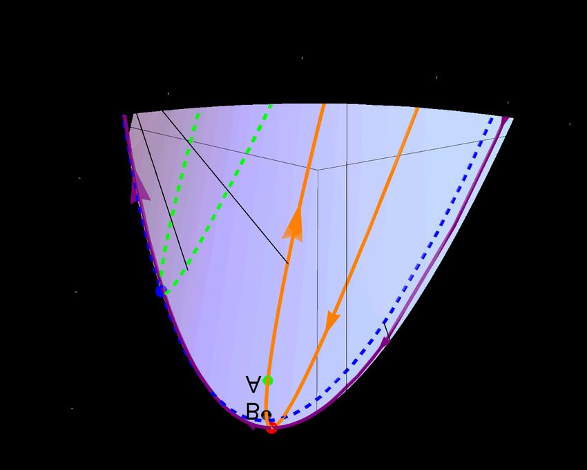
Entropy 2018, 20, 865 3 of 12
Σ
ec
1+ α et
ηe = η = 1 − τ (4)
1− Σ
1−
ec
(1−α)et
!
1 1−Σ ec τΣ
ec
Pe = 1−τ− − . (5)
τt
e (1 − α ) t
e α et
where ∼ refers to energy weighted by the heat output from the baseline Carnot cycle, Tc ∆S; and the
currents are obtained by dividing by the dimensionless total time et. According to the above stated
definition, the Ω function is given by Ω = 2P − Pmin − Pmax = 2 (2η − ηC ) Qh , whose dimensionless
form is
( 1 + τ ) 1 − Σ 2Σ
e = 1−τ −
ec ec
Ω − . (6)
τ et (1 − α) et2 α et2
The main results related to power output and Omega function maximization are presented.
In the LD-HE model τ and Σ e c do not play a role in the optimization, since Σ
e c involves intrinsic
properties of the device. For τ and Σc given, both MP and MΩ operation regimes accept global
e
optimization through α and et.
The values that maximize Pe and Ω e are [24]
r1
MP,
1− Σ
ec
1+
τΣ
α∗
ec
= 1 (7)
r MΩ,
(1+ τ ) (1− Σ
ec )
1+
2τ Σec
p p 2
2
τΣec + 1 − Σ MP,
ec
1− τ
et∗ = p r 2 (8)
2
2τ Σc + 1 − Σ c (1 + τ ) MΩ.
e e
1− τ
From now on, ∗ indicates the steady-state value at MP or MΩ conditions. As expected,
η MΩ ≥ η MP is obtained. Depending on the dissipation coefficient asymmetries, Σ
e c , both efficiencies
take values on the following intervals:
ηC ηC
≤ η MP ≤ , (9)
2 2 − ηC
3ηC 3 − 2ηC
≤ η MΩ ≤ η , (10)
4 4 − 3ηC C
where ηC = 1 − Tc /Th is the Carnot efficiency. The upper bounds are achieved in the limit Σe c → 0 and
the lower bounds when Σ e c → 1. In the symmetric case (Σe c = 1/2), both regimes efficiencies are:
sym p √
η MP = 1 − 1 − ηC = 1 − τ = ηCA , (11)
r r
sym (1 − ηC ) (2 − ηC ) τ (1 + τ )
η MΩ = 1 − = 1− , (12)
2 2
√
where the paradigmatic Curzon–Ahlborn efficiency, ηCA = 1 − Tc /Th , is obtained for the MP case.
On the other hand, efficiency and entropy production only accept optimization through α. For this
reason, the MΩ figure of merit represents a suitable choice to compare the dynamics toward relaxation
of the MP regime with another less entropy producing regime.Entropy 2018, 20, 865 4 of 12
3. Local Stability
As proposed in [20], the optimization variables α and et are dynamic variables governed via a
dynamic system that considers departures from the stationary state (operation regime). The restitution
forces are model as functions of Q
ė c and P.
e The currents associated to α and et are [20]:
dα
ė c (α, et) ,
= f Q (13)
dt
det
= g Pė(α, et) . (14)
dt
To guarantee stability, f and g must be monotonically decreasing functions fulfilling that in the
e c (α∗ , et∗ )) = g( Pe(α∗ , et∗ )) = 0. The simplest way to guarantee this [38–40] is by
stationary state f ( Q
assuming that the dynamics is described by the following linear ODE system with respect to Q ė c and P:
e
dα
ė c (α∗ , et∗ ) − Q
= C Q ė c (α, et) , (15)
dt
det
= D Pe(α∗ , et∗ ) − Pe(α, et) , (16)
dt
where C and D are positive constants and give the strength of the restitution forces, the larger they are,
the fastest the system will evolve.
In Figure 1, representative trajectories around the stationary state are plotted by solving
Equations (15) and (16). The main feature is the existence of a well defined basin of attraction
with a rich dynamics around the stable point. In Figure 1, three kind of curves are explicitly denoted.
The red curves evolve to the stationary state while the rest of the curves evolve to the nullcline where
dα
dt = 0, either from the left (dashed blue curves) or from the right (solid blue curves). A black curve is
shown as a representative case of a trajectory that surrounds the stability basin. The thermodynamics
behavior in the three kind of trajectories are by no means obvious, and the influence of time constraints,
as shown below, could indeed have relevant information on this regard.
In Figure 1, vertical and horizontal lines for constant values of α or et, respectively, are also explicitly
labeled in both cases. In Reference [41], it is shown that these time constraints reproduce open and
closed behaviors for the power vs. efficiency curves, typical from endoreversible (all irreversibilities
coming from the coupling to external heat thermal baths) and irreversible (including irreversibilities
coming from heat leaks and internal dissipation) heat engines. In Figure 1b, the evolution of the same
trajectories is shown in the α̇ vs. ėt plane. The endoreversible limit comprise the points where for the
same velocity in α, one obtains the smaller velocity in the operation time et (which is related to the
irreversibility of the system). Notice how, as the system evolves, the trajectories tend to reach the
endoreversible limit first, after that those evolving in the basin of attraction (red color) enter into a
dynamics bounded by the irreversible limit while some trajectories arriving as the nullcline (blue color)
can cross this limit.
The influence of the irreversible and endoreversible limits on the dynamic evolution of the system
are further addressed in the next section, which contains a thermodynamic analysis of the relaxation
trajectories to find the characteristic energetic behaviors associated with the basin of attraction.Entropy 2018, 20, 865 5 of 12
a) b)
8 0.06
Ωmax
7
6
˜ ̃
t t 0.03
5
Pmax
4
No HE
(P = 0) A
3
B
0
0.2 0.4 0.6 0.8 -0.02 0 0.02 0.04 0.06
α α
Figure 1. (a) Computed trajectories stemming from solving Equations (15) and (16) around the MP
and MΩ regimes. C = D = 1 and Σ e c = τ = 2/5 are used. The No HE label refers to the region
where P ≤ 0, represented by the shaded region. Blue continuous trajectories surround the basin of
attraction and arrive to the nullcline; a representative case of this is shown in black. Dashed blue curves
start at larger times and arrive to the nullcline from the left. Red lines are inside the basin of stability.
The constraints α = constant and et = constant are depicted in both regimes. They produce loop-like
and open curves in the P–η plane, respectively, which are typical for irreversible and endoreversible
heat engines, respectively. (b) The corresponding α̇ vs. ėt curves are depicted. The irreversible and
endoreversible limits are shown. The labels A and B on the irreversible limit correspond to the points
of minimum entropy production and maximum efficiency, respectively (see text for a more detailed
explanation). Arrows denote the evolution direction.
4. Entropy, Efficiency and Power Evolution Toward Relaxation
The role of entropy and internal energy as stability criteria in thermodynamics is well known.
In what appears a separate subject, the goal of optimization of energy converter is focused in obtaining
the larger efficiencies and power-output with the less entropy generation, with the simultaneous
optimization of the three quantities being an impossible task. In this section, we show that stability
favors, to some extent, the simultaneous optimization of the three thermodynamics functions.
By solving numerically Equations (15) and (16), the trajectories (α(t), et(t)) can be computed
and, by substituting them in Equations (3)–(5), the evolution of ∆S,
f η and Pe in the relaxation after a
e ∆S˙
perturbation on the system is obtained. These trajectories are depicted in Figure 2 over the η– P– f
surface. Figure 2a,b shows some of these trajectories around the MP state and Figure 2c,d shows some
trajectories around the MΩ state. The difference between Figure 2a,b is only the view point, the latter
making emphasis in the relation between entropy and efficiency. The same is done for Figure 2c,d for
the MΩ regime. As in Figure 1, blue continuous curves are those that go around the basin of attraction
and arrive to the nullcline dα
dt = 0, the black curve represents one of them, that orbits close to the stable
point but do not converge to it. The dashed trajectories involves perturbation where et > et MP andEntropy 2018, 20, 865 6 of 12
arrive to the nullcline from the opposite side. Red trajectories are inside the basin of attraction for the
MP state and they converge to the stationary state.
The dynamics around the MP stable point is such that, far from it, the solid blue curves evolve
toward the upper values of Pe in trajectories of increasing efficiency and decreasing entropy (more
noticeable in Figure 2b). The curves start to orbit states of larger power while moving to the true
MP state. In these oscillations, there are drops of power and efficiency and an increment of entropy.
After one last oscillation that misses the stable point, the curves decay toward the nullcline in a
trajectory where power output and efficiency decrease, and entropy production increases, finally
ending in the no-HE region where the power output and efficiency are negative.
b)
MP
0.35
η
0.3
0.25
0.1
̃ 0.15
ΔS
d)
0.48 MΩ
η
0.44
0.4
0.04 0.05
̃ 0.06
ΔS
˙
e ∆S
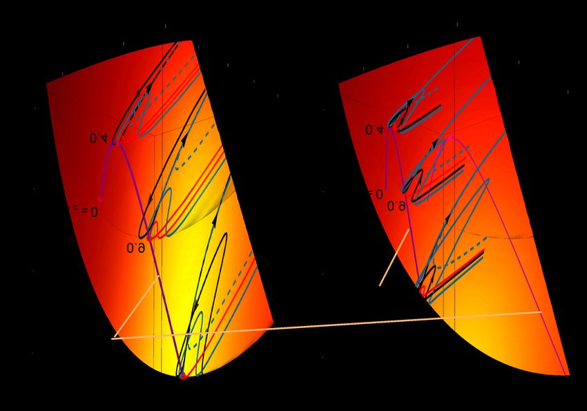
Figure 2. By solving Equations (15) and (16), we obtained trajectories on the (η, P, f ) space.
The depicted trajectories stem from the parameterization appearing in Figure 1. The color and
line-type codes are the same to distinguish different behaviors from the phase space. (a) The case
of MP regime; (b) the same trajectories are shown but emphasizing the relation between entropy
production and efficiency; (c) the MΩ case is shown; and (d) the corresponding figure highlighting the
entropy production vs. efficiency. In all cases, the trajectories evolve toward the cusp in each surface.
τ=Σ e c = 0.4 are used.
On the other hand, the dashed blue curves are such that they enter directly into the nullcline.
The trajectories inside the basin of attraction follow the same dynamic as the blue curves but they
present one small oscillation with a small power and efficiency drop and they rather enter into an orbit
that quickly drives them to the stable point. These small drops of power and efficiency and very small
increment of entropy, which only occurs close to the stable point, could be indeed the true difference
between the states inside the basin of attraction and those states that evolve toward the nullcline.
The dynamics on the MΩ regime follows a very similar pattern, as depicted in Figure 2c,d.
The evolution of the curves still present oscillations over values of the power output, even whenEntropy 2018, 20, 865 7 of 12
the fixed point is not the MP. A distinctive feature is that the trajectories are more lined and with a
narrower basin of attraction. Notice that, when comparing with the MP results, the MΩ regime implies
smaller entropy production trajectories and higher efficiency, in agreement with the bounds accounted
for Equations (9) and (10) for high asymmetries and Equations (11) and (12) for the symmetric case.
Notice in Figure 2c,d the different scales in entropy and efficiency with respect to Figure 2a,b
Therefore, all the above provides a firm basis to consider that stability could be linked to a
˙
e ∆S,
compromise of performance among η, P, f in what we can call a thermodynamic “self-improvement”
in the process of relaxation, with the smallest possible fluctuations on the performance of the engine.
An interesting feature results from comparing the relaxation trajectories with the open
(endoreverversible) and closed (irreversible) behaviors depicted in Figure 3a, where the irreversible
˙
e ∆S-η,
and endoreversible limits are displayed over the surface P- f in continuous lines for the MP state
and in dashed lines for the MΩ state. Both curves cross at the MP state, however, the irreversible limit
displays, additionally, points of minimum entropy production (labeled as A) and maximum efficiency
(labeled as B). The orientation of the arrows indicate the direction at which either α or et increase (from
0 to 1, and from 1 to ∞, respectively). It can be noticed that these times constraints are not arbitrarily
located with respect to the trajectories on the basin of attraction.
As explained above, regarding Figure 1b, far from the stable point, all trajectories tend to reach the
endoreversible limit (given by the constraint α = α Pmax ), while, near the stationary state, the trajectories
are bounded by the irreversible limit given by et = et Pmax . The reason for this is a hierarchy/distinction in
the relaxation behavior due to a thermodynamic self improvement attached to the stability dynamics.
In the linear approximation (near the stationary state), it was obtained that the stability depends only
on the relaxation of α [24], corresponding to the time constraint depicted in Figure 1a (horizontal line
with et = et Pmax ). Thus, trajectories in the basin of attraction are bounded by the irreversible limit; on the
other hand, far from the stationary state, the trajectories display a preference for the endoreversible
limit, which offers a number of advantageous features.
The preference to evolve toward the endoreversible limit can be understood by looking into
Figure 3b–f which apply for the MP regime (although the results are also valid for the MΩ state).
In Figure 3b, the endoreversible limit denote the lower value of heat waste for any given heat input.
In Figure 3c,d, the endoreversible limit gives the larger power and efficiency for a given entropy
production. Figure 3e,f shows that, additionally, it gives the lower entropy production for given heat
output and input, respectively. Thus, the system evolution reveals a preference for a better compromise
displayed by the endoreversible configuration, and the time constraints influence in a major way the
dynamics toward relaxation.
Next, the influence of the asymmetries keeping a fixed thermal gradient it is presented.
e ∆S˙
Figure 4 shows the η, P, f surfaces for three cases of Σ e c = {0.4, 0.9, 0.99} and for all possible values
of α ∈ (0, 1) and t ∈ (0, 50); in Figure 4a for MP and in Figure 4bfor MΩ. Over the depicted surfaces
e
lies the curve of MP states for all Σc ∈ (0, 1) (purple curve). The three MP states Σ e c = {0.4, 0.9, 0.99}
represented in the figure have their own dynamics toward the stable point. Some representative
trajectories are displayed over each surface. In this figure, it is noticeable that relaxation trajectories are
more likely to evolve in the direction of increasing power and efficiency and decreasing entropy. Those
arriving to the stable point, as stated above, have the smallest variations in entropy and efficiency,
while all the trajectories arriving to the nullcline evolve to states of less power, less efficiency and larger
entropy production. Thus, systematically in the search for the true MP, the orbits around the stable
point always search for more “convenient” thermodynamic states. It can be also seen in Figure 4 how
larger values of Σe c produce narrower basins of attraction, thus yielding trajectories with less variations
of power output, efficiency and entropy production. The MΩ states, in comparison with MP states,
have a better energetic evolution (less drops) but with the cost of having more constrained states.
Finally, Figure 5 shows the difference on the dynamics when different thermal gradients are
considered. As τ decreases the surface where the evolution is held diminish its area and the trajectoriesEntropy 2018, 20, 865 8 of 12
are more leaned. As the thermal gradient is larger, the basin of attraction accepts larger perturbations
but the nature of the trajectories is the same.
Figure 3. (a) The resulting endoreversible and irreversible behaviors, produced by the time constraints
˙
α = constant and et = constant, respectively, are depicted in a P–η–∆S f surface; in continuous lines for
MP and in dashed lines for MΩ. (b) Q ė h vs. − Q
ė c is shown. (c,d) The power and efficiency evolution,
respectively, as a function of the entropy generation. (e,f) The evolution of entropy production as the
output and input heat vary due to the relaxation dynamics. (b–f) The endoreversible limit clearly offers
a better compromise in the use of energy. τ = Σe c = 0.4 are used. (b–f) Plots for the MP regime.Entropy 2018, 20, 865 9 of 12
Figure 4. Dynamics described by Equations (15) and (16): local-stability of the MP state (a); and the MΩ
e ∆S˙
state (b) over the surfaces (η, P, f ) for three cases of Σ
e c = {0.4, 0.9, 0.99} with τ = 0.4. The surfaces
with larger Σc ’s contains those with smaller values of Σc . Over these surfaces lies the curve of all MP
e e
states for Σ
e c ∈ (0, 1). In all cases, the trajectories evolve with oscillations over the cuspid.
Figure 5. Relaxation evolution for (τ = {0.3, 0.5}) and for the two operation regimes. The curves of all
MP and MΩ states for Σ e c ∈ (0, 1) are shown. C = D = 1 and Σ e c = 0.9 are used.
5. Conclusions
The analysis of the dynamics behind local stability of operation regimes, such as maximum
power and maximum Ω functions, reveals a feature that recently has started to gain certain attention:
stability/constancy of heat devices should be considered as an additional ingredient in the optimizationEntropy 2018, 20, 865 10 of 12
of heat devices; and there exists a kind of trade-off among stability, power output and efficiency. Here,
the entropy production is added as another relevant aspect to consider.
It has been found that, for irreversible processes obeying the small dissipation assumption,
the stability basin is associated with thermal behaviors of simultaneous improvement of the main
thermodynamics quantities, power, efficiency and entropy, as well as small drops of their performance.
A comparison of the relaxation trajectories with the open and closed P vs. η behaviors of endoreversible
and irreversible heat engines reveals that, far from the stable point, the trajectories tend to evolve to
the endoreversible limit case, while, close to the stable point, the evolution occurs inside the region
delimited by the irreversible limit behavior, and all trajectories crossing this boundary will diverge to a
non-physical state. These qualitative behaviors apply for every value of the dissipation coefficient Σ ec
and for any thermal gradient, given by τ, although small numerical differences can be observed for
concrete numerical values of these parameters.
Author Contributions: The authors contributed equally to the paper. All authors have read and approved the
final manuscript.
Funding: This research was funded by Conacyt-MÉXICO Grant No. FC-1132. Universidad de Salamanca Contract
No. 2017/X005/1 and Junta de Castilla y Leon under project SA017P17.
Acknowledgments: M.S. acknowledges financial support from Conacyt-MÉXICO Grant No. FC-1132. J.G.A.
acknowledges Universidad de Salamanca Contract No. 2017/X005/1. M.J.S., A.C.H., and J.M.M.R. acknowledge
partial financial support from Junta de Castilla y Leon under project SA017P17.
Conflicts of Interest: The authors declare no conflict of interest.
References
1. Sánchez-Orgaz, S.; Pedemonte, M.; Ezzatti, P.; Curto-Risso, P.L.; Medina, A.; Calvo Hernández, A.
Multi-objective optimization of a multi-step solar-driven Brayton plant. Energy Convers. Manag. 2015,
99, 346–358. [CrossRef]
2. Sciubba, E.; Zullo, F. A Novel Derivation of the Time Evolution of the Entropy for Macroscopic Systems in
Thermal Non-Equilibrium. Entropy 2017, 19, 594. [CrossRef]
3. Curzon, F.; Ahlborn, B. Efficiency of a Carnot engine at maximum power output. Am. J. Phys. 1975, 43, 22.
[CrossRef]
4. Angulo-Brown, F. An ecological optimization criterion for finite-time heat engines. J. Appl. Phys. 1991, 69,
7465–7469. [CrossRef]
5. Esposito, M.; Kawai, R.; Lindenberg, K.; Van den Broeck, C. Efficiency at maximum power of low-dissipation
Carnot engines. Phys. Rev. Lett. 2010, 105, 7150603. [CrossRef] [PubMed]
6. Long, R.; Liu, Z.; Liu, W. Performance optimization of minimally nonlinear irreversible heat engines and
refrigerators under a trade-off figure of merit. Phys. Rev. E 2014, 89, 062119. [CrossRef] [PubMed]
7. Tu, Z.C. Stochastic heat engine with the consideration of inertial effects and shortcuts to adiabaticity.
Phys. Rev. E 2014, 89, 052148. [CrossRef] [PubMed]
8. Izumida, Y.; Okuda, K.; Roco, J.M.M.; Calvo Hernández, A. Heat devices in nonlinear irreversible
thermodynamics. Phys. Rev. E 2015, 91, 052140. [CrossRef] [PubMed]
9. Rui L.; Wei L. Unified trade-off optimization for general heat devices with nonisothermal processes.
Phys. Rev. E 2015, 91, 042127. [CrossRef]
10. Rui L.; Wei L. Ecological optimization for general heat engines. Phys. A Stat. Mech. Appl. 2015, 434, 232–239.
[CrossRef]
11. Zhang, Y.; Huang, C.; Lin, G.; Chen, J. Universality of efficiency at unified trade-off optimization. Phys. Rev. E
2015, 93, 032152. [CrossRef] [PubMed]
12. Singh V.; Johal, R.S. Feynman’s Ratchet and Pawl with Ecological Criterion: Optimal Performance versus
Estimation with Prior Information. Entropy 2017, 19, 576. [CrossRef]
13. Iyyappan, I.; Ponmurugan, M. Thermoelectric energy converters under a trade-off figure of merit with
broken time-reversal symmetry. J. Stat. Mech. 2017, 093207. [CrossRef]
14. Ye, Z.; Hu, Y.; He, J.; Wang, J. Universality of maximum-work efficiency of a cyclic heat engine based on a
finite system of ultracold atoms. Sci. Rep. 2017, 7, 6289. [CrossRef] [PubMed]Entropy 2018, 20, 865 11 of 12
15. Bejan, A.; Mamut, E. Thermodynamic Optimization of Complex Energy Systems; Springer Science & Business
Media: Berlin, Germany, 2012; ISBN 9401146853.
16. Avval, H.B.; Ahmadi, P.; Ghaffarizadeh, A.R.; Saidi, M.H. Thermo-economic–environmental multiobjective
optimization of a gas turbine power plant with preheater using evolutionary algorithm. Int. J. Energy Res.
2011, 35, 389–403. [CrossRef]
17. Lucia, U.; Grazzini, G. The Second Law Today: Using Maximum-Minimum Entropy Generation. Entropy
2015, 17, 7786–7797. [CrossRef]
18. Lucia, U.; Açıkkalp, E. Irreversible thermodynamic analysis and application for molecular heat engines.
Chem. Phys. 2017, 494, 47–55. [CrossRef]
19. Iyyappan, I.; Ponmurugan, M. General relations between the power, efficiency, and dissipation for the
irreversible heat engines in the nonlinear response regime. Phys. Rev. E 2018, 97, 012141. [CrossRef]
[PubMed]
20. Reyes-Ramírez, I.; Gonzalez-Ayala, J.; Calvo Hernández, A.; Santillán, M. Local-stability analysis of a
low-dissipation heat engine working at maximum power output. Phys. Rev. E 2017, 96, 042128. [CrossRef]
[PubMed]
21. Gonzalez-Ayala, J.; Santillán, M.; Reyes-Ramírez, I.; Calvo Hernández, A. Link between optimization and
local stability of a low dissipation heat engine: dynamic and energetic behaviors. Phys. Rev. E 2018,
98, 032142. [CrossRef]
22. Viktor, H.; Artem, R. Maximum efficiency of low-dissipation heat engines at arbitrary power. J. Stat. Mech.
2016, 073204. [CrossRef]
23. Calvo Hernández, A.; Medina, A.; Roco, J.M.M. Time, entropy generation, and optimization in low-dissipation
heat devices. New J. Phys. 2015, 17, 075011. [CrossRef]
24. Gonzalez-Ayala, J.; Calvo Hernández, A.; Roco, J.M.M. From maximum power to a trade-off optimization of
low-dissipation heat engines: Influence of control parameters and the role of entropy generation. Phys. Rev. E
2017, 95, 022131. [CrossRef] [PubMed]
25. Sekimoto, K.; Sasa, S. Complementarity Relation for Irreversible Process Derived from Stochastic Energetics.
JPSJ 1997, 66, 3326–3328. [CrossRef]
26. Schmiedl, T.; Seifert, U. Efficiency at maximum power: An analytically solvable model for stochastic heat
engines. Europhys. Lett. 2008, 81, 20003. [CrossRef]
27. Izumida, Y.; Okuda, K. Efficiency at maximum power of minimally nonlinear irreversible heat engines.
Europhys. Lett. 2012, 97, 10004. [CrossRef]
28. Guo, J.; Cai, L.; Yang, H.; Lin, B. Performance characteristics and parametric optimizations of a weak
dissipative pumped thermal electricity storage system. Energy Convers. Manag. 2017, 157, 527–535. [CrossRef]
29. Guo, J.; Wang, J.; Wang, Y; Chen, J. Efficiencies of two-level weak dissipation quantum Carnot engines at the
maximum power output. J. Appl. Phys. 2013, 113, 143510. [CrossRef]
30. Gonzalez-Ayala, J.; Roco, J.M.M.; Medina, A.; Calvo-Hernández, A. Carnot-Like Heat Engines Versus
Low-Dissipation Models. Entropy 2017, 19, 182. [CrossRef]
31. Johal, R.S. Heat engines at optimal power: Low-dissipation versus endoreversible model. Phys. Rev. E 2017,
96, 012151. [CrossRef] [PubMed]
32. Singh, V.; Johal, R.S. Feynman-Smoluchowski engine at high temperatures and the role of the constraints.
J. Stat. Mech. 2018, 2018, 073205. [CrossRef]
33. Yu-Han, M.; Xu, D.; Dong, H.; Chang-Pu, S. Universal constraints for efficiency and power of a
low-dissipation heat engine. Phys. Rev. E 2018, 98, 042112. [CrossRef]
34. Rojas-Gamboa, D. A.; Rodríguez, J. I.; Gonzalez-Ayala, J. ; Angulo-Brown, F. Ecological efficiency of finite-time
thermodynamics: A molecular dynamics study. Phys. Rev. E 2018, 98, 022130. [CrossRef] [PubMed]
35. Bauer, M.; Brandner, K.; Seifert, U. Optimal performance of periodically driven, stochastic heat engines
under limited control. Phys. Rev. E 2016, 93, 042112. [CrossRef] [PubMed]
36. Pietzonka, P.; Seifert, U. Universal Trade-Off between Power, Efficiency, and Constancy in Steady-State Heat
Engines. Phys. Rev. Lett. 2018, 120, 190602. [CrossRef] [PubMed]
37. Holubec, V.; Ryabov, A. Cycling tames power fluctuations near optimum efficiency. Phys. Rev. Lett. 2018,
121, 120601. [CrossRef] [PubMed]
38. Stuki, J.W. Stability analysis of biochemical systems– A practical guide, Prog. Biophys. Mol. Biol. 1978, 33,
99–187. [CrossRef]Entropy 2018, 20, 865 12 of 12
39. Santillán, M.; Mackey, M.C. Dynamic stability versus thermodynamic performance in a simple model for a
Brownian motor. Phys. Rev. E 2008, 78. [CrossRef] [PubMed]
40. Santillán, M.; Maya, G.; Angulo-Brown, F. Local stability analysis of an endoreversible Curzon-Ahborn-Novikov
engine working in a maximum-power-like regime. J. Phys. D Appl. Phys. 2001, 34, 2068. [CrossRef]
41. Gonzalez-Ayala, J.; Calvo Hernández, A.; Roco, J.M.M. Irreversible and endoreversible behaviors of the
LD-model for heat devices: the role of the time constraints and symmetries on the performance at maximum
χ figure of merit. J. Stat. Mech. 2016, 2016, 073202. [CrossRef]
c 2018 by the authors. Licensee MDPI, Basel, Switzerland. This article is an open access
article distributed under the terms and conditions of the Creative Commons Attribution
(CC BY) license (http://creativecommons.org/licenses/by/4.0/).You can also read