Orientation Adaptive Minimal Learning Machine for Directions of Atomic Forces

Page created by Dave Navarro

IT & Technique

English

Like
Share
Embed
Fullscreen
Slides
Download HTML
Download PDF
Abuse

←

→

Page content transcription

If your browser does not render page correctly, please read the page content below

ESANN 2021 proceedings, European Symposium on Artificial Neural Networks, Computational Intelligence
and Machine Learning. Online event, 6-8 October 2021, i6doc.com publ., ISBN 978287587082-7.
Available from http://www.i6doc.com/en/.

Orientation Adaptive Minimal Learning
Machine for Directions of Atomic Forces
Antti Pihlajamäki1 , Joakim Linja2 , Joonas Hämäläinen2 , Sami Malola1 ,
Paavo Nieminen2 , Tommi Kärkkäinen2 and Hannu Häkkinen1,3 ∗

1- University of Jyväskylä - Department of Physics, Nanoscience Center
FI-40014 Jyväskylä, Finland
2- University of Jyväskylä - Faculty of Information Technology
FI-40014 Jyväskylä, Finland
3- University of Jyväskylä - Department of Chemistry, Nanoscience Center
FI-40014 Jyväskylä, Finland

Abstract. Machine learning (ML) force ﬁelds are one of the most com-
mon applications of ML in nanoscience. However, commonly these meth-
ods are trained on potential energies of atomic systems and force vectors
are omitted. Here we present a ML framework, which tackles the greatest
diﬃculty on using forces in ML: accurate prediction of force direction. We
use the idea of Minimal Learning Machine to device a method which can
adapt to the orientation of an atomic environment to estimate the direc-
tions of force vectors. The method was tested with linear alkane molecules.

1 Introduction
In computational studies of atomic and molecular systems there are two funda-
mental quantities: potential energy of the system and force vectors subjecting
to the atoms. In general, atomistic simulations produce output for both of these
quantities. The most accurate way to compute them is to use ab initio methods,
which are directly based on quantum mechanics. However, they are computa-
tionally demanding, which has risen the popularity of machine learning (ML)
tools. This is due to the ability of ML to imitate the results of the high-level
theoretical methods with lowered computational cost. Especially popular tools
are ML force ﬁelds, which estimate high-dimensional potential energy surfaces of
atomic systems [1]. These energy surfaces can be diﬀerentiated to get forces but
the training the methods focuses on potential energies and forces are omitted.
Training a ML method to predict forces, instead of potential energies, is
not simple. Chemical environments of the atoms are often presented using so-
called descriptors. They produce translation, rotation and permutation invariant
representations of the environment according to the chemical composition and
geometry of the system [2]. They make regression tasks more feasible than in
∗ This work was supported by Academy of Finland through the AIPSE research program

with grant 315549 to H.H. and 315550 to T.K., through the Universities Profiling Actions with
grant 311877 to T.K., and through H.H.’s Academy Professorship. Work was also supported
by ”Antti ja Jenny Wihurin rahasto” via personal funding to A.P.. Computations were done at
the FCCI node in the University of Jyväskylä (persistent identifier: urn:nbn:fi:research-infras-
2016072533).

529

the case of using the atomic coordinates. Descriptors are highly useful but they
are not suitable for predicting a rotation variant output, such as force directions,
without major adjustments. However, if the description is rotation variant, the
model would require large amounts of data to cover the orientation space.
We tackle the challenges above by utilizing the Minimal Learning Machine
(MLM) [3] framework to create an orientation adaptive method. The main input
is still an invariant description of a chemical environment. Output half of the
method adjusts the spacial orientation of the reference data, which enables it
to estimate force directions without having to cover the orientation space. Here
we focus on the directions of the forces. Predicting the norms of the forces is
a normal regression task, which can be handled with conventional ML methods
such as Ridge regression or artiﬁcial neural networks.

2 Theoretical basis of orientation adaptive MLM
The general idea of the method is similar to the original MLM, which relies on
separate handling of input and output spaces[3]. The force direction prediction
splits into three parts, which use the descriptions of the chemical environments,
coordinates of the atoms and unit force vectors. First, reference atomic coordi-
nates are ﬁtted on top of input coordinates, rotating reference unit force vectors
respectively. Next, Euclidean distances are measured between input and refer-
ence descriptions forming a distance matrix, which is used to predict the cosines
of angles between rotated reference force vectors and a force vector to be pre-
dicted. Finally, by minimizing the diﬀerence between real and predicted angles,
the direction of the force is found.

2.1 Training orientation adaptive MLM
Three types of data are used in training: described chemical environments
N ×dx
X = {xi }N i=1 ∈ R , cartesian coordinates of the atoms itselves and their
N ×(1+M )×3
M nearest neighbors Y = {yi }N i=1 ∈ R , and unit vectors pointing to
the directions of the forces V = {v̂i }i=1 ∈ RN ×3 . From this data K references
N
K×(1+M )×3
are selected forming Q = {qj }K j=1 ∈ R
K×dx
, S = {sj }Kj=1 ∈ R and
T = {tj }j=1 ∈ R
K K×3
respectively. In yi and si the ﬁrst rows are the positions
of the analyzed atoms itselves.
The angle between force vectors can be measured reliably only if associated
atomic neighborhoods are in the same spatial orientation, therefore reference
neighborhoods in S are aligned with the ones in Y. We used ﬁtting method
introduced by Arun et al.[4]. From point sets one calculates
1+M

Hi,j = (yi,k − yi,1 )T (sj,k − sj,1 ) (1)
k=1

where Hi,j ∈ R3×3 . Using Singular Value Decomposition (SVD) Hi,j = UΛWT
one can form a rotation matrix Ri,j = WUT . This aligns neighbor-atoms, when
the analyzed atom itself is translated to the origin. The optimal order of M

530

neighbor-atoms is not known, therefore
1+Mpermutations are tested and the success
1
of fitting is estimated as gi,j = 1+M k=1 |(yi,k − yi,1 ) − (sj,k − sj,1 )Ri,j |. The
permutation yielding the smallest gi,j is selected.
After SVD fitting, the matrices needed to train the model are formed. The
basic training of the weight matrix B ∈ RK×K is written as
−1 T
B = DTin Din Din Dout (2)
N ×K
where D∗ ∈ R are originally distance matrices in input and output spaces
[3]. In our case there are three different D∗ matrices: Dx = {|xi −qj |} containing
1
1+M
Euclidean distances between chemical descriptions, Dg = { 1+M k=1 |(yi,k −
yi,1 ) − (sj,k − sj,1 )Ri,j |} with the goodness values of the SVD fittings and Dc =
{v̂i · (t̂j Ri,j )} having the cosines of the angles between force vectors in V and
the rotated vectors of T. We use equation (2) to train two weight matrices,
Bg from goodness values of fittings and Bc from cosines. In both training
processes Din = Dx but the output side Dout matrix is substituted with Dc or
Dg respectively. The purpose of two weight matrices is to use one to predict
angles and another is used to determine reliability of the data points.
SVD fitting causes variation to Dc and Dg matrices, because configurations
might be difficult to fit together. This variation is behaving as a semi-random
noise, distribution of which is unclear. Hence, we used Huber regression to make
the model robust to outliers [5]. The idea is similar to the robust MLM by Gomes
et al. [6]. The columns of matrices Bc and Bg are optimized by giving Dx and
columns of Dc or Dg to Huber regressor. The regressor also produces intercept
values cj for every column of B to ensure that data is centered to origin. The
robustness of the method is determined by the Huber parameter ∈ [1, 2], where
1 is producing statistically the most robust model.

2.2 Prediction of output direction
The prediction takes a description x of the chemical environment and y set of
coordinates of neighbor-atoms as an input. Euclidean distances between x and
reference descriptions in Q are measured forming distance vector dx , which is
used to estimate cosines and SVD fitting successes. With normally trained model
this is simply d∗ = dx B∗ and with robust trained model it is d∗ = dx B∗ + c∗ ,
where c∗ contains intercept values. The reference points sets in S are SVD
fitted to y producing success values of fittings, which are saved to vector g, and
rotation matrices to operate reference vectors in T.
Only references for which gj − dg,j ≤ 0 are used to predict the direction.
Otherwise accuracy of the SVD fitting is not enough. Unit vector û pointing to
the predicted direction is found by minimizing loss function
2 2
dc,k − (t̂k Rk ) · û gk
min J(û) = − exp − − . (3)
û∈R3 σ1 σ2
k∈Γ
Here σ1 and σ2 are parameters defining the width and the depth of the contribu-
tions of the included references. Γ contains the indeces of the accepted references.

531

The optimization is done via Sequential Quadratic Programming (SQP). Initial
guess is always a vector pointing from the atom itself to its nearest neighbor.

3 Testing with alkanes
Linear alkane molecules with number of carbon atoms ranging from two to seven
were used as test systems. Thermal vibrations of the molecules were simulated
by running molecular dynamics (MD) using Density Functional Tight-Binding
(DFTB) code Hotbit to compute potential energies and forces [7]. For every atom
initial velocities were generated from Maxwell-Boltzmann distribution with tem-
perature of 750 K. A single run was 1000 MD steps (1 step = 1 configuration of
the molecule) with 1.5 fs time step. Chemical environments were described using
the Smooth Overlap of Atomic Positions (SOAP) [8] implemented in DScribe
package [2]. SOAP parameters were set to nmax = 6, lmax = 1 and cut-off radius
was 3.0 Å (for further details see corresponding references). For the SVD fitting
four nearest neighbors were used. The dataset was produced by two separate
MD runs from all molecules (6 × 2 × 1000 configurations, 2 × 27000 carbon en-
vironments, 2 × 66000 hydrogen environments). Features in SOAP descriptions
were min-max scaled into [0, 1] and training data of 7500 points was sampled
for both elements using RS-maximin [9, 10]. All training data points were saved
as reference points. The descriptions of the hydrogen and carbon atoms were
sampled separately and separate models were trained for both elements. For
both elements one regular and eleven robust models were trained. For robust
models Huber parameters were sampled evenly from the range [1, 2] with steps
of 0.1. The third set of MD runs was used as test data. For carbon models,
test data contained all data points from the third MD runs. For hydrogen, data
points from the every second configurations of the molecules were used. The
parameters in loss function (3) were σ1 = 0.25 and σ2 = 0.5. The performance
was measured with weighted averages of the angles between predicted and real
force vectors. The squared norms of the real force vectors were used as weights.
In Figure 1 A the weighted average angles are shown for different models.
Training errors of regular models are out of visualization range. For hydrogen
this training error is 1.3° and for carbon 7.4°. Horizontal lines, representing
the test errors of regular models, lie at 55.4° for carbon and 42.1° for hydrogen.
Adding robustness increases training errors but generality is improved. For
carbon all robust models are working better than the regular model, the best
one producing the weighted average angle of 47.2° with Huber parameter of 1.1.
For hydrogen the effect of robustness is not as clear as for carbon. Only three
most robust models show improvement and the best result with Huber parameter
1.0 is giving the weighted average angle of 38.3°. Panels D-G in Figure 1 show
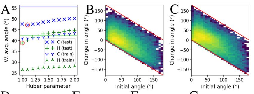
the test results for the regular models and the best robust models. In the case
of carbon the effect of robustness is not clear. The main improvements lie in the
region of large forces. For corresponding results for hydrogen effect is evident.
The directions of large forces have improved. The directions of the small forces
are difficult to handle, because even the tiniest movement of the atoms might

532

D E F G

Fig. 1: Performance of the method. Panel A shows the weighted average
angles between predicted and real directions. Lines show the test error of the
regular models and crosses correspond to the robust ones with the best test
results circled. Training errors of the regular models are below the visualization
range. B and C show the eﬀect of robustness from the best models of carbon and
hydrogen respectively as 2D histograms. Colors are logarithmically normalized.
Panels D-G show the test results. Colors present the density of the points.

totally change it. It is significantly more important to get correct directions for
the large forces than for small ones. For hydrogen the robust model is starting
to perform less well for small forces, which is seen as a different position of the
density maximum.
In Fig. 1 B and C the effect of added robustness is visualized. Horizontal
axes are the angles from the predictions with regular models. Vertical axes show
the difference φj − θj , where j ∈ [1, Ntest ], θj is a angle produced by the regular
model and φj is a corresponding angle from the best robust model. Negative
values correspond to improved predictions. Lower side red line shows the optimal
correction. Data is focusing to the lower region showing that robustness is
mostly improving predictions. For carbon in panel B this is clear, because data
is distributed close to the lower red line. For hydrogen improvement is modest.
The maximum region is spread significantly along horizontal direction (no effect)
and for small initial angles prediction have worsened but the main trend is
improving. A similar behavior can be seen in Fig 1 F and G.

533

ESANN 2021 proceedings, European Symposium on Artificial Neural Networks, Computational Intelligence
and Machine Learning. Online event, 6-8 October 2021, i6doc.com publ., ISBN 978287587082-7.
Available from http://www.i6doc.com/en/.

      4    Conclusions
      Orientation adaptive MLM shows great promise on force direction prediction.
      Its advantage is that it is not bound to full atomic structures but local chemical
      environments are enough. The shown accuracy is not perfect but it could be
      improved by optimizing its several parameters such as the ones of the SOAP
      descriptor, the loss function and the number of reference points. We are also
      working to improve the ﬁtting of atomic neighborhoods. A beautiful aspect of the
      method is that even after training the model, there are possibilities to aﬀect its
      accuracy by tailoring the loss function and the optimization method. The future
      applications of the method lie in atomic structure optimization and MD simu-
      lations. However, direction estimation is not only important in nanoscience but
      also in, for example, engineering wind power[11] and predicting stock market[12].
      Our method adds a new adjustable tool to tackle directional tasks.

      References
       [1] A. Pihlajamäki, J. Hämäläinen, J. Linja, et al. Monte Carlo Simulations of Au38(SCH3)24
           Nanocluster Using Distance-Based Machine Learning Methods. In J. Phys. Chem. A, vol.
           124 p. 4827–4836, 2020. doi:10.1021/acs.jpca.0c01512.
       [2] L. Himanen, M. O. J. Jäger, E. V. Morooka, et al. DScribe: Library of descriptors for
           machine learning in materials science. In Comput. Phys. Commun., vol. 247 p. 106949,
           2020. doi:10.1016/j.cpc.2019.106949.
       [3] A. H. de Souza Júnior, F. Corona, G. A. Barreto, et al. Minimal Learning Machine: A
           novel supervised distance-based approach for regression and classification. In Neurocom-
           puting, vol. 164 pp. 34 – 44, 2015. doi:10.1016/j.neucom.2014.11.073.
       [4] K. S. Arun, T. S. Huang, and S. D. Blostein. Least-Squares Fitting of Two 3-D
           Point Sets. In IEEE T. Pattern Anal., vol. PAMI-9 pp. 698 – 700, 1987. doi:
           10.1109/TPAMI.1987.4767965.
       [5] P. J. Huber. Robust Statistics. John Wiley & Sons, Inc, New Jersey, USA, 1981. ISBN
           0-47141805-6.
       [6] J. P. P. Gomes, D. P. P. Mesquita, A. L. Freire, et al. A Robust Minimal Learning
           Machine based on the M-Estimator. In ESANN 2017 proceedings, European Symposium
           on Artificial Neural Networks, Computational Intelligence and Machine Learning, pp.
           383–388. 2017.
       [7] P. Koskinen and V. Mäkinen. Density-functional tight-binding for beginners. In
           Comp. Mater. Sci., vol. 47(1) pp. 237 – 253, 2009.                 ISSN 0927-0256.     doi:
           10.1016/j.commatsci.2009.07.013.
       [8] A. P. Bartók, R. Kondor, and G. Csányi. On representing chemical environments. In
           Phys. Rev. B, vol. 87, 2013. doi:10.1103/PhysRevB.87.184115.
       [9] T. F. Gonzalez. Clustering to minimize the maximum intercluster distance. In Theor.
           Comput. Sci., vol. 38 pp. 293–306, 1985. doi:10.1016/0304-3975(85)90224-5.
      [10] J. Hämäläinen, A. S. C. Alencar, T. Kärkkäinen, et al. Minimal Learning Machine:
           Theoretical Results and Clustering-Based Reference Point Selection. In J. Mach. Learn.
           Res., vol. 21(239) pp. 1–29, 2020. URL http://jmlr.org/papers/v21/19-786.html.
      [11] Z. Tang, G. Zhao, and T. Ouyang. Two-phase deep learning model for short-term
           wind direction forecasting. In Renew. Energ., vol. 173 pp. 1005–1016, 2021. doi:
           10.1016/j.renene.2021.04.041.
      [12] M. Ballings, D. V. den Poel, N. Hespeels, et al. Evaluating multiple classifiers for stock
           price direction prediction. In Expert Syst. Appl., vol. 42 pp. 7046–7056, 2015. doi:
           10.1016/j.renene.2021.04.041.

                                                   534

You can also read