Parameterized Splitting of Summed Volume Tables
←
→
Page content transcription
If your browser does not render page correctly, please read the page content below
Eurographics Conference on Visualization (EuroVis) 2021 Volume 40 (2021), Number 3
R. Borgo, G. E. Marai, and T. von Landesberger
(Guest Editors)
Parameterized Splitting of Summed Volume Tables
Christian Reinbold and Rüdiger Westermann
Computer Graphics & Visualization Group, Technische Universität München, Garching, Germany
Abstract
Summed Volume Tables (SVTs) allow one to compute integrals over the data values in any cubical area of a three-dimensional
orthogonal grid in constant time, and they are especially interesting for building spatial search structures for sparse volumes.
However, SVTs become extremely memory consuming due to the large values they need to store; for a dataset of n values an SVT
requires O(n log n) bits. The 3D Fenwick tree allows recovering the integral values in O(log3 n) time, at a memory consumption
of O(n) bits. We propose an algorithm that generates SVT representations that can flexibly trade speed for memory: From similar
characteristics as SVTs, over equal memory consumption as 3D Fenwick trees at significantly lower computational complexity,
to even further reduced memory consumption at the cost of raising computational complexity. For a 641 × 9601 × 9601 binary
dataset, the algorithm can generate an SVT representation that requires 27.0GB and 46 · 8 data fetch operations to retrieve an
integral value, compared to 27.5GB and 1521 · 8 fetches by 3D Fenwick trees, a decrease in fetches of 97%. A full SVT requires
247.6GB and 8 fetches per integral value. We present a novel hierarchical approach to compute and store intermediate prefix
sums of SVTs, so that any prescribed memory consumption between O(n) bits and O(n log n) bits is achieved. We evaluate the
performance of the proposed algorithm in a number of examples considering large volume data, and we perform comparisons
to existing alternatives.
CCS Concepts
• Information systems → Data structures; • Human-centered computing → Scientific visualization;
1. Introduction in main memory. While the input field is only of size O(n), the
memory consumption of a SVT is of O(n log n).
Summed Area Tables (SATs) are a versatile data structure which Alternative SVT representations such as 3D Fenwick trees
has initially been introduced to enable high-quality mipmapping [Fen94, Mis13, SR17] offer a memory-efficient intermediate data
[Cro84]. SATs store the integrals over the data values in quadratic structure from which an adaptive space partition can be con-
areas of a two-dimensional orthogonal grid that start at the grid’s structed. 3D Fenwick trees have a memory consumption of O(n)
origin. The entries in a SAT can be considered prefix sums, as they bits, yet recovering the integral values requires a number of
are computed via column- and row-wise one-dimensional prefix O(log3 n) data fetch operations. For the example given in Fig. 1,
sums. With four values from a SAT the integral over any quadratic a 3D Fenwick tree requires only 27.5GB of memory, but to obtain
region can be obtained in constant time. The three-dimensional an integral value for a given volume 1512 · 8 fetches need to be
(3D) variant of SATs is termed Summed Volume Tables (SVTs). performed.
They are of special interest in visualization, since they can be used
For labelled datasets, SVTs can be used as an alternative to hier-
to efficiently build adaptive spatial search structures for sparse vol-
archical label representations like the mixture-graph [ATAS21], to
umes. In particular, construction methods for kD-trees and Bound-
efficiently determine the number of labels contained in a selected
ing Volume Hierarchies (BVHs) [VMD08, HHS06] can exploit
sub-volume. Furthermore, SVTs can effectively support a statis-
SVTs to efficiently find the planes in 3D space where the space
tical analysis of the data values in arbitrary spatial and temporal
should be subdivided.
sub-domains. As another application of SVTs, we briefly sketch
meteorological data analysis in Sec. 7. This includes the time- or
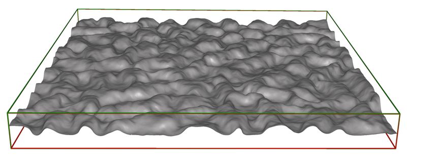
Fig. 1 shows a temperature snapshot in Rayleigh-Bénard con- memory-efficient computation of moving averages over selected
vection flow of size 641 × 9691 × 9601. To efficiently render this sub-regions and time intervals.
dataset via direct volume rendering algorithms, some form of adap-
tive spatial subdivision needs to be used to effectively skip empty
space. However, the SVT from which such an acceleration struc- 1.1. Contribution
ture can be computed requires 247.6GB of memory, so that only We propose an algorithm to generate SVT representations that can
on computers with large memory resources all data can be stored flexibly trade speed for memory. These representations build upon
© 2021 The Author(s)
Computer Graphics Forum © 2021 The Eurographics Association and John
Wiley & Sons Ltd. Published by John Wiley & Sons Ltd.C. Reinbold & R. Westermann / Parameterized Splitting of Summed Volume Tables
1x • a capacity estimator for the memory and compute requirements
1x n1 x of a given parameter tree,
n2 x
• a heuristic that automatically provides a parameter tree that
3x matches a prescribed capacity.
n3 x
Precision
Count
7x n4 x We analyze our proposed approach with respect to memory
consumption and data fetch operations, and compare the results
7x n5 x
to those of alternative SVT representations. By using differently
28x n6 x sized datasets, we demonstrate lower capacity requirements and
improved scalability of our approach compared to others.
The paper is structured as follows: We first discuss approaches
Figure 1: Schematic operation principle of splitting SVTs. A 3D ar- related to ours in the light of memory consumption and computa-
ray is hierarchically split into multiple high to low precision arrays tional issues. After a brief introduction to the concept of SATs, we
(decreasing color saturation indicates decreasing precision), to ob- introduce the versatile data structure our approach builds upon. We
tain a data structure from which sums over axis-aligned subarrays demonstrate in particular the parameterization of this data structure
can be computed. For the 641×9601×9601 input volume obtained to enable trading memory consumption for computational access
by a supercomputer simulation of a Rayleigh–Bénard convection, efficiency. In Sec. 6, we then describe how to realize a concrete
the SVT requires 247.6GB. Our algorithm generates SVT represen- SVT representation that adheres to a user defined performance or
tations at 27.0GB or 71.2GB, requiring respectively 46 or 8 data memory budget. We evaluate our design choices and compare the
fetch operations per prefix sum. obtained representations to alternative approaches in Sec. 7. We
conclude our work with ideas for future work.
2. Related Work
a recursive uni-axial partitioning of the domain and corresponding
partial prefix sums, in combination with a hierarchical representa- SATs have been introduced by Crow [Cro84], as a data struc-
tion that progressively encodes this information. Since partial pre- ture to quickly obtain integral values over arbitrary rectangular
fix sums require less bits to encode their values, the overall mem- regions in 2D data arrays. Since then, SATs have found use in
ory consumption can be controlled by the number and position of many computer vision and signal processing tasks such as ob-
the performed domain splitting operations. By using different par- ject detection [BTVG06, VJ04, GGB06, Por05], block matching
titioning strategies, any prescribed memory consumption between [FLML14], optical character recognition [SKB08] and region fil-
O(n) bits and O(n log n) bits can be achieved. tering [HPD08, Hec86, BSB10].
In principle, the algorithm proceeds in two phases: Firstly, for In computer graphics, SVTs are used to realize gloss effects
every possible SVT representation of a given volume an abstract [HSC∗ 05], and in particular to accelerate the creation of spatial
parameter tree is constructed. This tree encodes the uni-axial split search structures for sparse scene or data representations. Havran et
operations in a hierarchical manner, and it allows estimating both al. [HHS06] build a BVH / SKD-Tree hybrid acceleration structure
the memory consumption of the resulting SVT representation and for mesh data by discretizing the 3D domain and finding kd-splits in
the required data fetch operations for computing an integral value. expected O(log log n). A SVT over the discretized domain is then
Secondly, the tree is translated into the concrete SVT representa- used to evaluate the split cost function in constant time. Similarly,
tion, by traversing the tree and performing the encoded operations. Vidal et al. [VMD08] propose to use SVTs to speed up cost func-
tion evaluations in a BVH construction process for voxelized vol-
To find a SVT representation according to a prescribed mem-
ume datasets. In their work, the cost function requires the computa-
ory consumption or number of fetches, we propose a heuris-
tion of bounding volumes over binary occupancy data. By running
tic that generates a parameter tree which adheres to a given re-
binary search on a SVT, this task can be solved in O(log n) in-
source budget. This heuristic provides a close-to-optimal parame-
stead of O(n3 ), where n is the side length of the volume. Ganter &
ter tree for arbitrary budgets, over the entire spectrum ranging from
Manzke [GM19] propose to use SVTs to cluster bounding volumes
memory-efficient yet compute-intense SVT representations to stan-
of small size before assembling them bottom-up into a BVH for
dard memory-exhaustive SVT representations with constant recon-
Direct Volume Rendering (DVR). SVTs also allow to compute sta-
struction time.
tistical quantities for arbitrarily large axis-aligned regions in con-
Our algorithm generates SVT representations with equal mem- stant time [PSCL12]. Thus, they facilitate interactive exploratory
ory consumption as 3D Fenwick trees at significantly lower com- tasks in large scale volume datasets. The major drawback of SVTs
putational complexity. For the example in Fig. 1, we can construct is their memory consumption. Since prefix sums may span up to n
a SVT representation that requires 27.0GB but requires only as few elements, where n is the number of entries in a d-dimensional ar-
as 46 · 8 data fetch operations to retrieve an integral value, a de- ray, SVT entries require up to O(log n) bits precision. This yields a
crease in data fetch operations of 97% compared to Fenwick trees. total memory consumption of O(n log n), where the original array
Our specific contributions are is only of size O(n).
• an abstract parameter tree representation that translates directly In Computer Graphics, classical Mip Mapping [Wil83] (or Rip
into a SVT representation, Mapping in the anisotropic case) has been used for decades to ap-
© 2021 The Author(s)
Computer Graphics Forum © 2021 The Eurographics Association and John Wiley & Sons Ltd.C. Reinbold & R. Westermann / Parameterized Splitting of Summed Volume Tables
proximately compute partial means (or equivalently sums) of tex- to 30%. However, total memory consumption still is in O(n log n)
tures in constant time and O(n) memory. Partial means of boxes and does not scale well.
with power of two side length are precomputed and then interpo-
lated to approximate boxes with arbitrary side length. Belt [Bel08] 3D Fenwick Trees as introduced by Mishra [Mis13] have bene-
proposes to apply rounding by value truncation to the input array ficial properties with regard to both memory consumption and ac-
before computing its corresponding SVT. By reducing the preci- cess. As shown by Schneider & Rautek [SR17], they require O(n)
sion of the input, the SVT requires less bits of precision as well. To memory while allowing to compute prefix sums by summing up
compensate for rounding error accumulation, the rounding routine O(log3 n) values. In the 1D case [Fen94] this is achieved by recur-
is improved by considering introduced rounding errors of neigh- sively processing subsequent pairs of numbers such that the first
boring SVT entries. Clearly, this scheme cannot be used to reduce number is stored verbatim; and the second one is summed up with
memory requirements for arrays of binary data. Although approx- the first one and then passed to the next recursion level. In the 3D
imate schemes may suffice for imaging or computer vision tasks case, this process generalizes to processing 23 -shaped blocks where
where small errors usually are compensated for, they are inappro- one corner is stored verbatim and the other corners are processed
priate in situations where hard guarantees are required (e.g. the sup- recursively. Note that a complexity of O(log3 n) still yields num-
port of a BVH has to cover all non-empty regions). bers in the thousands for n ≥ 10243 and above. Our approach im-
proves significantly in this regard.
Exact techniques such as computation through the overflow
Memory Efficient Integral Volume (MEIV) by Urschler et al.
[Bel08] or the blocking approach by Zellmann et al. [ZSL18] en-
[UBD13] first computes the full SVT and then partitions it into
force a maximal precision bound per SVT entry and, thus, avoid
bricks of small size (brick sizes of 33 up to 123 were investigated).
the logarithmic increase in memory. The former approach simply
For each brick, MEIV stores its smallest prefix sum bo together
drops all except for ` least significant bits and hence stores prefix
with a parameter µ describing a one-parameter model for the brick
sums modulo 2` . As long as queried boxes are small enough such
entries subtracted by bo. The value of µ is determined by an opti-
that partial sums greater or equal than 2` are omitted, this method
mization step performing binary search. Since the model cannot fit
is exact. This approach excels in filtering tasks with kernels of pre-
all block entries perfectly, the remaining error per entry is stored
scribed box size. However, it is not applicable in situations where
in a dynamic word length storage with smallest as possible preci-
box sizes are either large or not known in advance.
sion. As a result, MEIV is able to decrease memory consumption
Zellmann et al., on the other hand, brick the input array into exceptionally well with regard to the minimal overhead of fetching
323 bricks and compute a SVT for each brick separately, hence only two values from memory, namely some brick information and
they dub their method Partial SVT. As each prefix sum cannot sum a value from the dynamic word length storage. Its clear downside is
over more than 323 elements, the amount of additional bits per en- the increased construction time by fitting µ. In the authors’ exper-
try is limited to 15 bits. However, when computing sums along iments, constructing the MEIV representation with optimal block
boxes which do not fit into a single 323 brick, one value has to size for the largeRandomVolume dataset takes 75 times longer than
be fetched from memory for each brick intersecting the queried for the regular SVT. Further, MEIV cannot give any memory guar-
box. Since there still are O(n/(323 )) = O(n) many bricks, this ap- antees as the final memory consumption is sensitive to the chosen
proach scales equally poorly as summing up all values by iterating brick size as well as the actual dataset. Compared to MEIV, we ob-
over the input array directly. More generally, any attempt to store tain the same savings in memory by allowing 6 instead of 2 fetches
intermediate sums with a fixed precision PREC scales poorly. In from memory, and—more importantly—memory requirements of
order to recover the "largest" possible sum of all array elements, our approach are known before actual encoding. Further, our ap-
one would have to add up at least O(n)/2PREC factors of maximal proach is able to flexibly adapt memory requirements in the full
size 2PREC . To circumvent this issue, the authors propose to build range of O(n) to O(n log n) respecting the user’s need, and thus
a hierarchical representation of partial SVTs where the largest en- still can be used whereas other approaches (especially Ehsan and
tries of each partial SVT form a new array that again is bricked and MEIV) run out of memory.
summed up partially. However, the authors admit that all bricks that
overlap only partially with the queried box have to be processed at
their current hierarchy level. Hence, the number of touched bricks 3. Summed Volume Tables
reduces to the size of the box boundary. In the best case of cubes
as boxes, the complexity still is O(n2/3 )—which is impractical for We now briefly describe the basic concept underlying SVTs. For
n ≥ 10243 . the sake of clarity, we do so on the example of a SAT, the 2D coun-
terpart of a SVT, before we extend the concept to an arbitrary num-
Ehsan et al. [ECRMM15] propose a technique that allows to ber of dimensions. Note that we use 1-based indexing whenever
compute arbitrary prefix sums by fetching a constant number of accessing arrays during the course of the paper.
four values only through replacing each third row and column of
Given a two-dimensional array F of scalar values, an entry (x, y)
a 2D array by their corresponding high precision SAT entries. By
of its corresponding SAT is computed by summing up all values
either adding an array entry to preceding SAT entries, or subtract-
contained in the rectangular subarray that is spanned by the indices
ing it from subsequent ones, the full SAT can be recovered. Their
(1, 1) and (x, y), that is
approach directly generalizes to 3D, requiring eight values instead.
As a consequence, they only have to store 19 out of 27 SVT entries SATF [x, y] := ∑ F[x0 , y0 ].
in high O(log n) precision, reducing memory consumption by up x0 ≤x, y0 ≤y
© 2021 The Author(s)
Computer Graphics Forum © 2021 The Eurographics Association and John Wiley & Sons Ltd.C. Reinbold & R. Westermann / Parameterized Splitting of Summed Volume Tables
If the values of a SAT are precomputed, partial sums of F for
Fa
arbitrary rectangular subarrays can be computed in constant time, 1 0 0 0 1 0 1 0 1 1 1 2 1 0 0 1 0 1 1 1
0 0 0 1 0 1 0 0 0 0 1 1 1 2 0 0 0 0 0 1 0 1 0 0 1
by making use of the inclusion-exclusion principle. Instead of read- 1 0 1 0 0 1 0 0 1 1 0 0 2 1 1 4
1 0 1 0 1
0 1 0 0 1 1 0 0
1 1 1 0 1
ing and adding up values of F along the whole region spanned by 1 0 1 0 0 1 0 0 1 1 1 0 2 1 310 0 1 100 1 0 110 1 1 0
1 2 1 0 1
(x1 + 1, y1 + 1) and (x2 , y2 ), it suffices to read the SAT-values at the 1 1 1 1 1 1 0 0 0 1 0 0 4 2 211 1 1 011 1 0 001 1 0 0
1 2 0 0 1
0 0 0 1 0 1 0 1 1 1 0 1 2 00 0 0 00 1 0 01 1 0
corners of the selected subarray. It holds that 1 3 0 1 1
0 1 0 1 1 0 1 1 0 1 2 3 0 1 0 1 0 1 0 1
F[x0 , y0 ] = SATF [x1 , y1 ] + SATF [x2 , y2 ]− Fs0 Fs1 Fs2
∑
x1C. Reinbold & R. Westermann / Parameterized Splitting of Summed Volume Tables
1 0 0 0 1 0 1 0 1 1 3x 1x
0 0 0 1 0 1 0 0 0 0 1
1 0 1 0 0 1 0 0 1 1 0 0
2. dim (y)
)
1
(z
1 0 1 0 0 1 0 0 1 1 1 0
m
1
1 1 1 1 1 1 0 0 0 1 0 0
di
3.
1
0 0 0 1 0 1 0 1 1 1 0
1
1. dim (x) 0 1 0 1 1 0 1 1 0 1
(a) 2x 2x
1 2 2x 1 0 0 1 1
1 1 2 0 0 0 0 0 0 1
2 1 1 4 1 0 1 0 1 1 1 0 0
1 1 1
2 1 3 0 1 0 1 1 0 1 1 1 0
2 1 1
4 2 2 1 1 1 1 0 1 0 1 0 0 (b)
2 0 1
0 2 0 0 0 0 0 1 1 0 0 0 4x
3 0 1 0 0 0
2 3 0 1 0 0 1 0 0 0 0
0
0 0 0 0
0
0 0 0 0
0
0 0 0
2x 2 0 1 4x 0 0 1
0 0
0
1 1 1 1 0 0 0 1
2 1 2 1 1 0 1 0 0 (c) pad
2 0
2 1 2 0 0 1 0
0
I = {2} 0 1 0 I = {2,3} Figure 4: Splitting a 13 × 4 × 3 array along the longest dimension
I = {1,2,3}
I = {Ø} into subarrays of size 3 with (a) at_end, (b) distributed and (c) pad
1x 8 7 1x 8 6
alignment. Split positions are highlighted on the left. The number
5 6 7 5 5 6
8 8 6 5
2x 2 0 1 4x 0 0 2
2 4 5 4
8 1 1 1 1 0 1 1 2 4 and shape of resulting subarrays is shown on the right.
8 8 5 1 2 1 2 1 1 0 1 1 1 2 4 4 2
7 2 1 3
6 7 2 1 2 1 2 0 0 1 1 1 3 2 1
5 0 2
0 5 0 0 1 0 1 2 1
3 1
2 3 0 1
Memory
at_end: The last subarray remains "incomplete" and thus has a
Figure 3: Sample split hierarchy of a 10 × 4 × 3 binary input ar- size smaller than z along the split dimension.
ray. We show aggregate arrays and subarrays generated during the distributed: A slice is removed from as many subarrays as one
recursive split process. Whenever two or more subarrays of similar would have to pad in order to expand the last subarray to size z
shape form in a split operation, a multiplier in the top left corner of along the split dimension.
a block indicates how many arrays of its shape arise. The block’s pad: The last subarray is padded with zeros until size z is reached.
filling with numbers matches the first (i.e. leftmost/undermost) of
Figure 4 depicts the results of all alignment strategies when split-
its associated subarrays. The other subarrays of similar shape may
ting a 13 × 3 × 3 field with fixed subarray size of 3 along the first
contain different numbers. As a final step indicated by wavy ar-
dimension. During our experiments we noticed no difference in
rows, each terminal array is processed by computing cumulative
quality when generating SVT representations with either at_end or
sums according to the leaf parameter I (see Sec. 4.1). The result is
distributed aligned splits. Further, both yield subarrays of at most
stored in memory.
two different shapes, thus restricting the branching factor of the re-
cursion to 3. Pad alignment incurs an additional memory overhead
of up to 10%. In return it guarantees a unique subarray shape, re-
ducing the branching factor to 2. This property may be favourable
parameter subtree representing its subsequent split process is built when engineering massively parallel en- & decoding schemes in
and attached to the root node. If a newly acquired array is terminal, future work. In the scope of this paper we decided to utilize dis-
a leaf node describing its memory layout is created and attached tributed aligned splits.
instead.
In summary, a split now is defined by the split dimension k and
In a naive implementation, the parameter quickly becomes un- subarray size z that allows to infer the split positions according to
manageable since it is branching with a factor that scales with the the distributed alignment strategy. Both values are encoded into an
number of subarrays per split. By recursively splitting all subar- internal tree node representing the split. A leaf node, on the other
rays of similar shape in the same way, one can collapse all of their hand, contains a set of dimension indices I ⊆ {1, . . . , d} which de-
corresponding subtrees to a single one and thus reduce the branch- scribe along which dimensions array values are cumulated before
ing factor to the number of different subarray shapes occurring in finally storing each cumulated value in memory. The special cases
a split, plus one for the aggregate array. Hence, we constrain the of storing verbatim or SVT entries are represented by I = ∅ and
branching factor by requiring as few as possible different subarray I = {1, . . . , d}, respectively. Fig. 5 shows the parameter tree de-
shapes. This can be achieved by specifying a fixed subarray size scribing the split hierarchy of Fig. 3. Note that a tree node may
z along the split dimension and placing split positions accordingly represent more than one array by collapsing subtrees of similarly
with equal spacing. However, we have to resolve alignment issues shaped subarrays. For instance, two arrays of shape 3 × 4 × 3 are
if z + 1 is not a divisor of the length nk of the split dimension mi- represented by the "k= 2, z= 1" internal node, and the memory lay-
nus one. Overall, we experimented with three different alignment out of the four terminal arrays of shape 3 × 1 × 3 is given by the
strategies: "I = {1,2,3}" node.
© 2021 The Author(s)
Computer Graphics Forum © 2021 The Eurographics Association and John Wiley & Sons Ltd.C. Reinbold & R. Westermann / Parameterized Splitting of Summed Volume Tables
k = 1, z = 3
1 0 0 0 1 0 1 0 1 1 3 1 0 0 1 0 1 0 1 1
0 0 0 1 0 1 0 0 0 0 1 2 3 0 0 0 0 0 1 0 0 0 0 0 1
1 0 1 0 0 1 0 0 1 1 0 0 3 2 51 0 1 0 1 0 1 0 1 10 1 1 0 0
1 3 613 0 1 1 100 1 0 0 100 1 1 1 1 0
1 0 1 0 0 1 0 0 1 1 1 0 3
1 6 213 1 1 1 001 1 1 1 100 0 1 1 0 0
1 1 1 1 1 1 0 0 0 1 0 0 6
1 2 00 0 0 0 00 1 0 0 01 1 1 1 0
I = {2} k = 2, z = 1 I = {2,3} 0 0 0 1 0 1 0 1 1 1 0
1
2
4 0 1 1
0 1 0 1 1 0 1 1 0 1 4 0 1 0 1 0 1 1 0 1
shift flip
Figure 6: Splitting a 10 × 4 × 3 array by permitting subtraction.
I=Ø I = {1,2,3} I=Ø Compared to Fig. 2, the first split position is introduced after two
subarrays instead of one, and the second (red) subarray is conju-
Figure 5: A parameter tree of depth 2 describing the split hierarchy gated by first shifting by one and then flipping. Note how the boxed
of Fig. 3. It has two internal (blue) and five leaf nodes (green). The 1 changes position. Subarrays in green are not conjugated.
leftmost subtree of each internal node describes the split hierarchy
of the aggregate array whereas the remaining subtrees describe the
split hierarchy of subarrays for two different subarray shapes. Text
a top-down-top traversal of the corresponding parameter tree de-
in nodes indicate encoded parameters. Note that the lower right
scribing the split hierarchy. When descending the tree, information
leaf node can be chosen arbitrarily since for the 3D shape given
about shapes and largest possible entries is propagated according
in Fig. 3 there is only one unique subarray shape arising from the
to the split parameters k, z. Note that whereas the largest possible
lower split.
entry for subarrays can be taken over from the array being split, for
aggregate arrays, an additional factor of 2z + 1 has to be applied.
It matches the number of values that are summed up to compute
4.2. The conjugate trick a single entry of the aggregate array when utilizing the conjugate
trick (see Sec. 4.2).
To reduce the numbers of split positions and thus the number of
high precision aggregates by one half (without changing the subar-
ray size), we are generalizing the technique described by Ehsan 5.1. Memory requirements
et al. [ECRMM15]. Instead of adding up a subarray prefix sum Let T be the parameter tree. If T consists of a single, terminal node
and the aggregate prefix sum at the preceding split position as in with dimension indices I, the largest possible entry that will be
Eq. (1), one can obtain the same result by subtracting the prefix stored in memory is given by m · ∏i∈I ni , where n is the array shape
sum of a flipped subarray from the aggregate prefix sum at the sub- at the terminal node and m is the array’s largest possible entry. Con-
sequent split position. If Fsi is the (i + 1)-th subarray with entries sequently, we have
Fsi [v] = F[v|k=ci +vk ], we denote with Fs∗i its conjugate that is ob-
tained by shifting by one and mirroring along the split dimension, MEM(T ) = |n| · dlog2 (1 + m · ∏ ni )e.
i∈I
i.e. Fs∗i [v] = F[v|k=ci+1 +1−vk ]. Then we have
SVTF [v] = SVTFa [v |k=i ] − SVTFs∗ [v |k= j ], (2) If the root node of T is an internal node, let Ta be the subtree
i−1
describing the representation of the aggregate array Fa , and let Ts1
where i = min{m | cm ≥ vk } and j = ci − vk . and Ts2 be the two subtrees describing representations for the two
distinct subarray shapes. Then, the memory consumption can be
By replacing every second subarray by its conjugated version,
computed as
one out of two split positions become superfluous. An exemplary
split resulting from this process is shown in Fig. 6. Whenever a MEM(T ) = MEM(Ta ) + λ1 · MEM(Ts1 ) + λ2 · MEM(Ts2 ),
corner v is located in a subarray with odd index, Eq. (2) is used to
where λi is the number of subarrays with shape represented by Tsi .
compute the prefix sum, and Eq. (1) otherwise. If the last subarray
of a split is a conjugate one, a split position at nk (the last possible The memory required for storing the parameter tree itself is neg-
position) is added to ensure that a subsequent split position always ligible. Even for large datasets of GB-scale, the whole parameter
exists. Allowing for both addition and subtraction and thus halv- tree is of KB-size. If the parameter tree is fixed beforehand and
ing the size of Fa generally improves the final SVT representation baked into the encoding & decoding algorithm, it does not need to
by a more shallow split hierarchy and/or smaller block sizes at leaf be stored at all.
levels. This is advantageous as smaller SVT leafs require less pre-
cision per entry, and smaller verbatim leafs require less additions 5.2. Estimation of fetch operations
to obtain a prefix sum.
The parameter tree T exposes an upper bound for the number of
fetch operations required to compute a prefix sum. We call this
5. Analysis of the parameter tree bound the fetch estimate for T and denote it by FETCH(T ). If the
If the shape of the input array F as well as its largest possible en- root node of T is terminal with dimension indices I, we require
try (usually of the form 2#bits − 1) is known in advance, all rele- FETCH(T ) = ∏ ni
vant properties of a SVT representation of F can be derived via i∈{1,...,d}\I
© 2021 The Author(s)
Computer Graphics Forum © 2021 The Eurographics Association and John Wiley & Sons Ltd.C. Reinbold & R. Westermann / Parameterized Splitting of Summed Volume Tables
fetches to compute a prefix sum, with n being the array shape at the
Memory consumption
Memory consumption
terminal node. If the root node of T is internal, we have
FETCH(T ) = FETCH(Ta )+
(3)
max(FETCH(Ts1 ), FETCH(Ts2 ))
min
with the same notation as in Sec. 5.1. Since computing a pre-
fix sum according to Eq. (1, 2) is performed by querying a prefix min
sum of the aggregate array and one subarray, the fetch estimate is
an upper bound for the number of fetch operations—however, not Fetch count Fetch count
necessarily the minimal one. In the appendix, we present a method
for computing a tighter bound that in our experiments is lower by Figure 7: Schematic illustration of parameter tree search spaces.
3% on average and 24% at most. All fetch counts presented in this Each dot represents a parameter tree of certain fetch count and
paper are computed with the tighter bound instead of the fetch es- memory consumption. Optimal parameter trees are colored in
timate. green and define the memory-performance trade-off curve shown in
black. By restricting the search space in one quantity and optimiz-
A very coarse upper bound for the number of compute opera- ing for the other, the optimum is uniquely determined (highlighted
tions per prefix sum can be given by four times the number of dot).
fetches. Since memory access is of magnitudes slower than sim-
ple arithmetic operations, we conclude that computing prefix sums
is memory-bound. Hence, we use the number of fetch operations as
querying this search space for SVT representations yields a param-
performance indicator.
eter tree instance that minimizes both the fetch count and the mem-
ory consumption with respect to input arrays of fixed shape and
5.3. Update costs precision. However, representations with low fetch count have a
high memory consumption and vice versa. To obtain a well defined
Whenever a value of F is modified, a single aggregate of Fa as well
optimization problem, we restrict the search space to representa-
as one value of the subarray containing the modified value have
tions that do not exceed a prescribed budget of either the number
to be updated. Hence, the cost UPDATE(T ) for updating the SVT
of fetch operations or the memory consumption, and then ask for
representation can be described by the same recursion formula (3)
the SVT representation that minimizes the respective other quan-
as for the fetch estimate. At terminal nodes however, update costs
tity. The resulting parameter trees follow a memory-performance
are computed by
trade-off curve as shown in Fig. 7.
UPDATE(T ) = ∏ ni
The parameters which define a parameter tree are all discrete
i∈I
quantities, so that we are facing a combinatorial optimization prob-
since an entry of a terminal array of shape n can be part of up to lem. Even though we do not give a formal proof here, we believe
∏i∈I ni sums stored in memory. that this problem is NP-hard. Thus, we propose a heuristic H that
receives the shape n of the input array as well as a control parameter
5.4. Construction costs λ and returns a parameter tree H(λ, n) that is close to the mem-
ory-performance trade-off curve. Increasing [decreasing] λ typi-
In the supplement, we show that each value stored in memory by cally results in parameter trees with higher [lower] fetch count and
our SVT representation is a certain partial sum of the input array lower [higher] memory consumption. In particular, this design al-
F. Hence, all stored values can be efficiently determined by com- lows finding a beneficial parameter tree for a prescribed budget B
puting the classical SVT of F for instance via GPU computing, of either fetches or—more interestingly—memory. It is achieved
and then sampling a partial sum from the SVT for each stored by defining the function
value. Since our representation stores n values at leaf nodes, and (
SVTs can be computed in O(n) and sampled in O(1), the over- FETCH(H(λ, n)) − B if fetch budget
f (λ) =
all runtime-complexity of the construction algorithm is O(n). Due MEM(H(λ, n)) − B if memory budget
to the fundamental assumption that O(n log n) of main memory is
and applying a root-finding method such as the bisection method
not available, we propose to realize the classical SVT via bricking
to find λ with f (λ) ≤ 0 being close to zero. Then, H(λ, n) is a
strategies falling back to larger, but slower memory (e.g. persistent
parameter tree that, on the one hand, minimizes the unconstrained
storage). After construction, partial sums can be queried by fetch-
quantity, and exhausts the given budget on the other hand.
ing data from the constructed SVT representation that is stored in
(fast) main memory. In the algorithmic formulation of the heuristic, λ represents a
threshold for the fetch estimate described in Sec. 5.2. It is guar-
anteed that the fetch estimate of H(λ, n) does not exceed λ. We
6. Identification of optimal parameter trees
achieve this by the following procedure: If λ equals one, the heuris-
Our split hierarchy design opens up a high-dimensional search tic returns the parameter tree representing a classical SVT; that is
space for SVT representations, with the parameters trees being el- a single leaf node with I = {1, . . . , d}. If, on the other hand, λ is
ements in the space of parameters defining the hierarchy. Ideally, at least as large as the shape product |n|, it returns a single leaf
© 2021 The Author(s)
Computer Graphics Forum © 2021 The Eurographics Association and John Wiley & Sons Ltd.C. Reinbold & R. Westermann / Parameterized Splitting of Summed Volume Tables
node with setting I = ∅—that is the verbatim representation. For
1 < λ < |n|, the heuristic builds an internal node. The split di- 608KB
mension k is chosen such that nk = max(n1 , . . . , nd ). The subar-
ray size z is derived from λ according to an interpolation function
that is manually defined to match the structure of optimal param- 400KB
eter trees for small array shapes. These were computed once by a
Branch-and-Bound strategy that performs an exhaustive search.
200KB
The split parameters k and z define the shapes n(a) , n(s1 ) , n(s2 ) of
the aggregate array and the subarrays. Thus, we can use the heuris-
tic recursively to compute the subtrees of the internal node. To do 32KB
so, we define control parameters λa , λs and set the aggregate sub- 100 101 102 103 104 105
tree to H(λa , n(a) ) and both subarray subtrees to H(λs , n(s1 ) ) and
H(λs , n(s2 ) ) respectively. By requiring λa , λs ≥ 1 and λa + λs ≤ λ,
we assure that the recursion terminates and that the fetch estimate Figure 8: Memory-performance curves for a binary 643 volume,
of the final parameter tree does not exceed λ. This is due to Eq. (3) when (blue) solving the global combinatorial optimization prob-
and the assumption that the heuristic already satisfies this guaran- lem of parameter trees, and when (green) utilizing parameter trees
tee for recursive calls. In order to find a reasonable choice for λa returned by our heuristic. The x-axis shows number of fetch opera-
and λs , we again analyzed optimal parameter trees and noticed that tions. The y-axis shows memory consumption. Black lines indicate
the ratio of the fetch estimate FETCH(Ta ) of the aggregate subtree lower and upper bounds for the memory consumption of SVT rep-
to the fetch estimate FETCH(T ) of the whole tree correlates to the resentations.
ratio of the number of split positions (n(a) )k to the length nk of the
split dimension. While the latter ratio can be computed from the
split parameters, the first is unknown yet. However, by assuming 7.1. Quality of the heuristic
that the observed correlation applies for arbitrary array shapes, we
We now evaluate how closely the parameter trees returned by the
can derive an estimate for the first ratio. Now, the exact value for
heuristic match the optimal parameter trees. The optimal mem-
λa is obtained by matching λa /λ to the estimate of the first ratio.
ory-performance curve for a binary 643 volume is shown by the
Then, λs is computed by subtracting λa from λ. Pseudo code for
blue curve in Fig. 8. A point (x, y) on the curve indicates that there
the heuristic is given in the appendix.
exists an optimal parameter tree with x fetches and y bits of mem-
ory consumption, i.e., if memory is constrained to y bits, our hier-
archical data structure principally allows to reduce the number of
7. Evaluation required fetches to x, and vice versa. The green curve indicates the
The following evaluation sheds light on a) the quality of the heuris- characteristic of our proposed heuristic. By measuring the shift in
tic to find an optimal parameter tree (Sec. 6) and b) on the proper- x-direction, one can determine the fetch operation overhead of the
ties of our derived SVT representations compared to alternative ap- heuristic for a fixed memory threshold. Compared to the optimal
proaches, such as MEIV by Urschler et al. [UBD13], 3D Fenwick solution, roughly 1.5 times the optimal amount of fetches are re-
Trees by Mishra [Mis13], Partial SVTs by Zellmann et al. [ZSL18], quired. Note that due to the logarithmic scale of the x-axes, a shift
and the approach of Ehsan et al. [ECRMM15]. translates to a factor instead of an offset. Vice versa, measuring the
shift in y-direction yields the memory overhead of the heuristic, as-
All our experiments were run on a server architecture with 4x suming a fixed budget of fetches. Here we can clearly see that the
Intel Xeon Gold 6140 CPUs with 18 cores @ 2.30GHz each. Al- heuristic performs quite well except for the number of 4 fetches,
though we do not exploit any degree of parallelism, the genera- where memory consumption is increased by 25%.
tion of parameter trees with the proposed heuristic requires be-
Note that although the memory-performance curve given by the
tween 8.5s seconds for the smallest and 45.4s for the largest dataset
heuristic is not guaranteed to be monotone, it shows a clear falling
(see Table 1). Timings reflect convergence speed of the bisection
trend. Thus, when using the bisection method w.r.t. λ to achieve a
method used during parameter tree search as well as the cost for
certain memory threshold, close to perfect results can be expected.
evaluating the heuristic in each bisection step. Parameter tree gen-
We are also confident that the heuristic has not been manually over-
eration for single digit fetch counts is fast since the runtime of the
fitted to the validation scenario. In the design phase, optimal param-
heuristic correlates with the size of the parameter tree—and trees
eter trees for various 1D to 4D arrays with at most 9.000 elements
are very shallow in that scenario.
were investigated, while the volume used in the evaluation contains
As the parameter tree has to be created only once for a fixed ar- 262.144 elements. On the other hand, due to this we cannot ensure
ray shape and precision, we consider the runtime of the heuristic that the results of the evaluation generalize to GB-scale arrays.
as negligible. Finding globally optimal parameter trees, however, is
not tractable even for MB-scale datasets. The Branch-and-Bound
7.2. Comparative study
strategy for precomputing optimal parameter trees already takes
12.5 hours for a 643 dataset, clearly necessitating the use of a In this study, we compare the SVT representations found by our
heuristic. heuristic to the approaches proposed by Ehsan et al. [ECRMM15],
© 2021 The Author(s)
Computer Graphics Forum © 2021 The Eurographics Association and John Wiley & Sons Ltd.C. Reinbold & R. Westermann / Parameterized Splitting of Summed Volume Tables
Table 1: Performance statistics for various SVT representations. Each group of three rows contains results (memory consumption, fetch count)
for different approaches using the same volume. For each volume, theoretical lower and upper bounds for SVT representations are given.
The Reference column shows results for the reference approaches by others. The Ours columns show results and timings for parameter tree
computation for our SVT representations under varying constraints. Either memory or fetch count is constrained according to the reference
in the same row. Note that the non-constrained quantities (in bold) are significantly lower than the corresponding reference quantities.
Volume Reference Ours (Memory ≤ Ref. Memory) Ours (Fetch ≤ Ref. Fetch)
Name Memory Fetch Memory Fetch Timing Memory Fetch Timing
256 × 256 × 256 Ehsan 36.6MB 8 35.1MB 3 20ms 14.9MB 8 41ms
Size: 2MB Part. SVT 32MB 512 27.0MB 4 25ms 3.9MB 476 8.0s
SVT: 50MB Fen. Tree 8.0MB 512 8.0MB 38 8.5s 3.9MB 476 8.1s
1024 × 1024 × 1024 Ehsan 2.8GB 8 2.7GB 3 23ms 1.2GB 8 52ms
Size: 128MB Part. SVT 2GB 32K 1.5GB 5 147ms 170.1MB 27.5K 31.4s
SVT: 3.9GB Fen. Tree 511.6MB 1000 511.6MB 40 6.9s 252.7MB 952 20.5s
2048 × 2048 × 2048 Ehsan 24.3GB 8 24.2GB 3 26ms 10.3GB 8 56ms
Size: 1GB Part. SVT 16GB 256K 12.7GB 5 161ms 1.2GB 255.8K 33.5s
SVT: 34GB Fen. Tree 4.0GB 1331 4.0GB 39 9.7s 1.9GB 1294 17.3s
641 × 9601 × 9601 Ehsan 176.6GB 8 168.1GB 3 30ms 71.2GB 8 51ms
Size: 6.9GB Part. SVT 110.1GB 1.8M 86.7GB 5 157ms 7.5GB 1.7M 40.4s
SVT: 247.6GB Fen. Tree 27.5GB 1521 27.0GB 46 11.8s 11.8GB 1468 34.6s
8192 × 8192 × 8192 Ehsan 1.8TB 8 1.8TB 3 51ms 725.5GB 8 40ms
Size: 64GB Part. SVT 1TB 16M 892.8GB 5 100ms 67.9GB 10.6M 39.1s
SVT: 2.5TB Fen. Tree 256.0GB 2197 252.7GB 46 10.7s 114.4GB 2188 45.4s
Mishra [Mis13], Zellmann et al. [ZSL18] and Urschler et al. 3D array into subarrays of size 323 , so that empty subarrays can be
[UBD13]. Table 2 summarizes the qualitative features supported pruned and do not need to be stored. Even though the so generated
by the varying approaches. For a quantitative analysis, we manu- sparse structure requires a certain overhead to encode the sparsity
ally compute the memory consumption as well as the number of information, it is likely that at extreme sparsity levels the Partial
fetch operations for all reference methods except for Urschler et SVTs become competitive with respect to memory consumption. It
al., which will be covered later. We use binary volumes of shape is, on the other hand, not the case that the number of fetch opera-
2563 and 1K 3 , to reproduce the results of the alternatives from tions decreases similarly, since indirect memory access operations
other works. To demonstrate the scalability of our approach, ad- are required to step along the sparse encoding.
ditional results using large scale binary datasets from 2K 3 to 8K 3
Another comparison we perform is against MEIV of Urschler
are presented. The results of these experiments are given in Table 1.
et al. [UBD13], by reusing the array shapes and precision of the
They generalize to arrays with elements of arbitrary precision p, by
datasets used in the authors’ work. We set the lowest achieved
adding an offset of (p − 1) · n to all memory footprints of both our
memory consumption achieved by MEIV as fixed memory bud-
and reference methods.
get and compute the parameter tree according to Sec. 6. For the
It can be seen that our proposed heuristic performs significantly smallRandomVolume dataset of shape 5123 and a maximal possible
better than any other approach relying on intermediate sum com- entry of 1023 we require 6 fetch operations and 311MB of mem-
putation. In all cases, we can achieve an improvement of more than ory (compared to 319MB by MEIV). For the largeRandomVolume
a factor of 2.5 in memory consumption or number of fetch oper- dataset of shape 1K 3 and a maximal possible entry of 512 we
ations while matching the budget regarding the respective other again require 6 fetch operations, but 2491MB of memory (com-
quantity. Notably, while it seems that the approach by Ehsan is in pared to 2544MB by MEIV). In the case of the realCTVolume
all scenarios only this factor behind us, it cannot reduce the mem- dataset with shape 512 × 512 × 476 and a maximal possible entry
ory consumption any further. Thus, where Ehsan requires 1.8TB, of 1023, MEIV achieves roughly 350MB of memory consumption.
our SVT variant can go down as low as 64GB. In comparison to We achieve 304MB while requiring 5 fetch operations. Clearly, we
Partial SVTs, we can trade almost all fetch operations for the mem- achieve results of equal quality compared to MEIV without having
ory requirement of 67.9GB, and can reduce the memory require- its limitations as described in Sec. 2.
ment about more than 90% at the same number of fetch opera-
tions. Compared to the 3D Fenwick Tree, our SVT representation 7.3. Meteorological use case
requires only 2% of the number of fetch operations at similar mem-
ory consumption. In meteorological and climatological research, historical weather
data such as the publicly available ERA5 data set [HBB∗ 20] con-
It is fair to say, however, that the improvements over Partial taining global, atmospheric reanalysis data is often analyzed us-
SVTs with respect to memory requirement become less significant ing statistical measures like mean and variance over spatial sub-
with increasing sparsity of the volume. Partial SVTs first split the domains and time intervals. These measures indicate trends and can
© 2021 The Author(s)
Computer Graphics Forum © 2021 The Eurographics Association and John Wiley & Sons Ltd.C. Reinbold & R. Westermann / Parameterized Splitting of Summed Volume Tables
Table 2: Properties of different SVT representations where n is the number of data values in the volume. Besides memory consumption, we
show runtime-complexities for reconstructing an arbitrary partial sum, reconstructing an actual data value, single-threaded construction
of the data structure, and updating the representation after a single data value is changed. Further, we indicate if memory consumption
can be predicted before constructing the representation, if construction is straightforwardly parallelizable, and if representations can be
modified to exploit sparsity in datasets. For our approach, we present lower and upper complexity bounds for all achievable representations.
(*) Average runtime-complexity is shown. Worst Case complexity is O(log3 n). (**) Our approach reconstructs data values with the same
amount of fetches as required for partial sum reconstruction by regarding data values as partial sums over hyperboxes of size 1. (***) Update
performance heavily depends on the actual parameter tree (see Sec. 5.3).
Verbatim SVT Ehsan Part. SVT Fen. Tree MEIV Ours
O(n) O(n log n)
Memory consumption O(n) O(n log n) O(n log n) O(n) O(n) – O(n log n)
large const. better in practice
O(n)
Read partial sum O(n) O(1) O(1) O(log3 n) O(1) O(1) – O(n)
small const.
Read data value O(1) O(1) O(1) O(1) O(1) * O(1) O(1) – O(n) **
O(n)
Construction time – O(n) O(n) O(n) O(n) O(n)
large const.
3
Data value update O(1) O(n) O(n) O(1) O(log n) O(n) O(1) – O(n) ***
Predictable memory
X X X X X x X
consumption
Parallelizable construction – X X X X X X
Can exploit sparsity X x x X x x ?
be used to reveal correlations between observed physical quantities In the future, we intend to address the following issues: Firstly,
at different sub-domains and times. we will engineer cache-aware and/or GPU-accelerated encoding
As a use case, we utilize the 2m temperature field of the ERA5 and decoding schemes, so that a) decoding can further benefit from
hourly data on single levels from 1979 to 2020 [HBB∗ 18]. Data massive parallelism and b) encoding can be realised in timings sim-
is rescaled to 8bit integers according to Sec. 4 and hourly data ilar to state-of-the-art SAT encoding. [CWT∗ 18, EFT∗ 18, HSO07]
is aggregated per day, yielding an 8bit precision dataset of size Secondly, we will apply our approach to build spatial acceleration
1440 × 721 × 15404. We use our parameterized SVT representa- structures such as BVHs for large-scale mesh or volume datasets.
tion to plot the mean temperature progressions over different in- Further, we plan to efficiently build implicit BVH structures for
teractively selected, spatial sub-domains of 150 × 50 grid points DVR that optimize for low variance in density per bounding vol-
(roughly matching the extend of the Sahara) in a line plot. Assum- ume. By using the technique described by Phan et al. [PSCL12],
ing a horizontal resolution of 200 pixels, we partition the user cho- our technique allows to compute variances in constant time with-
sen time range in 200 equally large intervals and compute one ag- out running out of memory. Note that memory efficient SVT im-
gregate for each pixel. When viewing the whole temporal domain, plementations are especially important in this regard, because the
each aggregate thus describes a sub-domain of 150 × 50 × 77 grid SVT that is used for computing second order moments is created
points and requires 577.500 fetches from the verbatim dataset of from an input of double precision than the dataset. Third, we will
size 14.9GB. A SVT requires only 8 fetch operations but 78.2GB investigate potential optimizations for sparse data. Here we will ad-
of memory. In contrast, by employing our parameterized SVT rep- dress how much memory used by our data structure can be saved by
resentation using 22.8GB of memory, we can still perform the com- pruning empty subarrays, and whether the heuristic can be adapted
putation of mean values per any sub-domain using 31 · 8 fetch op- to respect empty regions in the dataset.
erations, facilitating an interactive visual analysis of arbitrary sub-
regions. Further, we plan to extend our approach to nominal data, that is,
computing SVTs of histograms instead of scalar entries. Applica-
tions are in any research field processing segmented volumes such
8. Conclusion and future work as neuroscience or material science. For instance, Al-Thelaya et
We have proposed a versatile data structure and heuristic for gener- al. [ATAS21] perform sub-volume queries over nominal data to en-
ating SVT representations that can flexibly trade speed for memory. able real-time computation of local histograms over user selected
Hence, SVT representations that are specifically built for a fixed regions. However, due to arranging histograms in a Mip Map struc-
memory or compute budget can be utilized. In a number of experi- ture, their approach requires an additional footprint assembly step
ments on large scale datasets we have compared the resulting SVT that quickly becomes unfeasible if very large regions are selected.
representations to those by others, and we have demonstrated sig- By replacing the Mip Map architecture with our SVT scheme, we
nificantly reduced memory consumption at similar decoding per- believe it will be possible to build a sophisticated mixture graph
formance, or vice versa. that allows to skip the footprint assembly step entirely.
© 2021 The Author(s)
Computer Graphics Forum © 2021 The Eurographics Association and John Wiley & Sons Ltd.C. Reinbold & R. Westermann / Parameterized Splitting of Summed Volume Tables
References L UPU C., R ADNOTI G., DE ROSNAY P., ROZUM I., VAMBORG F.,
V ILLAUME S., T HÉPAUT J.-N.: The era5 global reanalysis. Quar-
[ATAS21] A L -T HELAYA K., AGUS M., S CHNEIDER J.: The Mixture terly Journal of the Royal Meteorological Society 146, 730 (2020),
Graph-A Data Structure for Compressing, rendering, and querying seg- 1999–2049. URL: https://rmets.onlinelibrary.wiley.
mentation histograms. IEEE Transactions on Visualization and Com- com/doi/abs/10.1002/qj.3803, arXiv:https://rmets.
puter Graphics 27, 2 (2021), 645–655. doi:10.1109/TVCG.2020. onlinelibrary.wiley.com/doi/pdf/10.1002/qj.3803,
3030451. 1, 10 doi:https://doi.org/10.1002/qj.3803. 9
[Bel08] B ELT H. J. W.: Word Length Reduction for the Integral Im- [Hec86] H ECKBERT P. S.: Filtering by Repeated Integration. SIG-
age. In 15th IEEE International Conference on Image Processing (2008), GRAPH Comput. Graph. 20, 4 (Aug. 1986), 315–321. doi:10.1145/
pp. 805–808. doi:10.1109/ICIP.2008.4711877. 3 15886.15921. 2
[BSB10] B HATIA A., S NYDER W. E., B ILBRO G.: Stacked Integral [HHS06] H AVRAN V., H ERZOG R., S EIDEL H.: On the Fast Construc-
Image. In IEEE International Conference on Robotics and Automation tion of Spatial Hierarchies for Ray Tracing. In IEEE Symposium on In-
(2010), pp. 1530–1535. doi:10.1109/ROBOT.2010.5509400. 2 teractive Ray Tracing (2006), pp. 71–80. doi:10.1109/RT.2006.
[BTVG06] BAY H., T UYTELAARS T., VAN G OOL L.: SURF: Speeded 280217. 1, 2
Up Robust Features. In Computer Vision – ECCV 2006 (Berlin, Heidel- [HPD08] H USSEIN M., P ORIKLI F., DAVIS L.: Kernel Integral Images:
berg, 2006), Leonardis A., Bischof H., Pinz A., (Eds.), Springer Berlin A Framework for Fast Non-Uniform Filtering. In IEEE Conference on
Heidelberg, pp. 404–417. 2 Computer Vision and Pattern Recognition (2008), pp. 1–8. doi:10.
[Cro84] C ROW F. C.: Summed-Area Tables for Texture Mapping. In 1109/CVPR.2008.4587641. 2
Proceedings of the 11th Annual Conference on Computer Graphics and [HSC∗ 05] H ENSLEY J., S CHEUERMANN T., C OOMBE G., S INGH M.,
Interactive Techniques (New York, NY, USA, 1984), SIGGRAPH ’84, L ASTRA A.: Fast Summed-Area Table Generation and its Applications.
Association for Computing Machinery, p. 207–212. doi:10.1145/ Computer Graphics Forum 24, 3 (2005), 547–555. doi:10.1111/j.
800031.808600. 1, 2 1467-8659.2005.00880.x. 2
[CWT∗ 18] C HEN P., WAHIB M., TAKIZAWA S., TAKANO R., M AT- [HSO07] H ARRIS M., S ENGUPTA S., OWENS J. D.: Parallel prefix sum
SUOKA S.: Efficient Algorithms for the Summed Area Tables Primi- (scan) with CUDA. GPU gems 3, 39 (2007), 851–876. 10
tive on GPUs. In IEEE International Conference on Cluster Computing
(CLUSTER) (2018), pp. 482–493. doi:10.1109/CLUSTER.2018. [Mis13] M ISHRA P.: A New Algorithm for Updating and Querying Sub-
00064. 10 arrays of Multidimensional Arrays. arXiv (2013). arXiv:1311.
6093v6. 1, 3, 8, 9
[ECRMM15] E HSAN S., C LARK A. F., R EHMAN N. U., M C D ONALD -
M AIER K. D.: Integral Images: Efficient Algorithms for Their Compu- [Por05] P ORIKLI F.: Integral Histogram: A Fast Way to Extract His-
tation and Storage in Resource-Constrained Embedded Vision Systems. tograms in Cartesian Spaces. In IEEE Computer Society Conference
Sensors 15, 7 (2015), 16804–16830. doi:10.3390/s150716804. on Computer Vision and Pattern Recognition (CVPR’05) (2005), vol. 1,
3, 6, 8 pp. 829–836 vol. 1. doi:10.1109/CVPR.2005.188. 2
[EFT∗ 18] E MOTO Y., F UNASAKA S., T OKURA H., H ONDA T., [PSCL12] P HAN T., S OHONI S., C HANDLER D. M., L ARSON E. C.:
NAKANO K., I TO Y.: An Optimal Parallel Algorithm for Computing Performance-Analysis-Based Acceleration of Image Quality assessment.
the Summed Area Table on the GPU. In IEEE International Parallel In IEEE Southwest Symposium on Image Analysis and Interpretation
and Distributed Processing Symposium Workshops (IPDPSW) (2018), (2012), pp. 81–84. doi:10.1109/SSIAI.2012.6202458. 2, 10
pp. 763–772. doi:10.1109/IPDPSW.2018.00123. 10 [SKB08] S HAFAIT F., K EYSERS D., B REUEL T. M.: Efficient Imple-
[Fen94] F ENWICK P. M.: A New Data Structure for Cumulative Fre- mentation of Local Adaptive Thresholding Techniques Using Integral
quency Tables. Software: Practice and Experience 24, 3 (1994), 327– Images. In Document Recognition and Retrieval XV (2008), Yanikoglu
336. doi:10.1002/spe.4380240306. 1, 3 B. A., Berkner K., (Eds.), vol. 6815, International Society for Optics and
Photonics, SPIE, pp. 317 – 322. doi:10.1117/12.767755. 2
[FLML14] FACCIOLO G., L IMARE N., M EINHARDT-L LOPIS E.: Inte-
gral Images for Block Matching. Image Processing On Line 4 (2014), [SR17] S CHNEIDER J., R AUTEK P.: A Versatile and Efficient GPU Data
344–369. doi:10.5201/ipol.2014.57. 2 Structure for Spatial Indexing. IEEE Transactions on Visualization and
Computer Graphics 23, 1 (2017), 911–920. doi:10.1109/TVCG.
[GGB06] G RABNER M., G RABNER H., B ISCHOF H.: Fast Approxi- 2016.2599043. 1, 3
mated SIFT. In Computer Vision – ACCV 2006 (Berlin, Heidelberg,
2006), Narayanan P. J., Nayar S. K., Shum H.-Y., (Eds.), Springer Berlin [UBD13] U RSCHLER M., B ORNIK A., D ONOSER M.: Memory Effi-
Heidelberg, pp. 918–927. 2 cient 3D Integral Volumes. In Proceedings of the IEEE International
Conference on Computer Vision (ICCV) Workshops (June 2013). 3, 8, 9
[GM19] G ANTER D., M ANZKE M.: An Analysis of Region Clustered
BVH Volume Rendering on GPU. Computer Graphics Forum 38, 8 [VJ04] V IOLA P., J ONES M. J.: Robust Real-Time Face Detection. In-
(2019), 13–21. doi:10.1111/cgf.13756. 2 ternational Journal of Computer Vision 57, 2 (2004), 137–154. 2
[HBB∗ 18] H ERSBACH H., B ELL B., B ERRISFORD P., B IAVATI G., [VMD08] V IDAL V., M EI X., D ECAUDIN P.: Simple Empty-Space Re-
H ORÁNYI A., M UÑOZ , S ABATER J., N ICOLAS J., P EUBEY C., R ADU moval for Interactive Volume Rendering. Journal of Graphics Tools 13,
R., ROZUM I., S CHEPERS D., S IMMONS A., S OCI C., D EE D., T HÉ - 2 (2008), 21–36. doi:10.1080/2151237X.2008.10129258. 1,
PAUT J.-N.: ERA5 hourly data on single levels from 1979 to present,
2
2018. Copernicus Climate Change Service (C3S) Climate Data Store [Wil83] W ILLIAMS L.: Pyramidal Parametrics. In Proceedings of the
(CDS). Accessed on 08-03-2021. doi:10.24381/cds.adbb2d47. 10th Annual Conference on Computer Graphics and Interactive Tech-
10 niques (New York, NY, USA, 1983), SIGGRAPH ’83, Association for
[HBB∗ 20] H ERSBACH H., B ELL B., B ERRISFORD P., H IRAHARA Computing Machinery, p. 1–11. doi:10.1145/800059.801126.
S., H ORÁNYI A., M UÑOZ -S ABATER J., N ICOLAS J., P EUBEY C., 2
R ADU R., S CHEPERS D., S IMMONS A., S OCI C., A BDALLA S., [ZSL18] Z ELLMANN S., S CHULZE J. P., L ANG U.: Rapid kd Tree Con-
A BELLAN X., BALSAMO G., B ECHTOLD P., B IAVATI G., B ID - struction for Sparse Volume Data. In Proceedings of the Symposium on
LOT J., B ONAVITA M., D E C HIARA G., DAHLGREN P., D EE D., Parallel Graphics and Visualization (Goslar, DEU, 2018), EGPGV ’18,
D IAMANTAKIS M., D RAGANI R., F LEMMING J., F ORBES R., Eurographics Association, p. 69–77. 3, 8, 9
F UENTES M., G EER A., H AIMBERGER L., H EALY S., H OGAN R. J.,
H ÓLM E., JANISKOVÁ M., K EELEY S., L ALOYAUX P., L OPEZ P.,
© 2021 The Author(s)
Computer Graphics Forum © 2021 The Eurographics Association and John Wiley & Sons Ltd.You can also read