Super Star Clusters in the Central Starburst of NGC 4945 - IOPscience
←
→
Page content transcription
If your browser does not render page correctly, please read the page content below
The Astrophysical Journal, 903:50 (24pp), 2020 November 1 https://doi.org/10.3847/1538-4357/abb67d
© 2020. The Author(s). Published by the American Astronomical Society.
Super Star Clusters in the Central Starburst of NGC 4945
Kimberly L. Emig1 , Alberto D. Bolatto2 , Adam K. Leroy3 , Elisabeth A. C. Mills4 , María J. Jiménez Donaire5 ,
Alexander G. G. M. Tielens1,2 , Adam Ginsburg6 , Mark Gorski7 , Nico Krieger8 , Rebecca C. Levy2 ,
David S. Meier9,10 , Jürgen Ott10 , Erik Rosolowsky11 , Todd A. Thompson3 , and Sylvain Veilleux2
1
Leiden Observatory, Leiden University, P.O. Box 9513, 2300-RA Leiden, The Netherlands; emig@strw.leidenuniv.nl
2
Department of Astronomy and Joint Space-Science Institute, University of Maryland, College Park, MD 20742, USA
3
Department of Astronomy, The Ohio State University, 140 West 18th Avenue, Columbus, OH 43210, USA
4
Department of Physics and Astronomy, University of Kansas, 1251 Wescoe Hall Drive, Lawrence, KS 66045, USA
5
Observatorio Astronómico Nacional, Alfonso XII 3, E-28014, Madrid, Spain
6
Department of Astronomy, University of Florida, P.O. Box 112055, Gainesville, FL, USA
7
Chalmers University of Technology, Gothenburg, Sweden
8
Max-Planck-Institut für Astronomie, Königstuhl 17, D-69120 Heidelberg, Germany
9
Department of Physics, New Mexico Institute of Mining and Technology, 801 Leroy Place, Socorro, NM 87801, USA
10
National Radio Astronomy Observatory, P.O. Box O, 1003 Lopezville Road, Socorro, NM 87801, USA
11
Department of Physics, 4-183 CCIS, University of Alberta, Edmonton, AB T6G 2E1, Canada
Received 2020 May 4; revised 2020 August 24; accepted 2020 September 5; published 2020 October 30
Abstract
The nearby (3.8 Mpc) galaxy NGC 4945 hosts a nuclear starburst and Seyfert type 2 active galactic nucleus
(AGN). We use the Atacama Large Millimeter/submillimeter Array (ALMA) to image the 93 GHz (3.2 mm)
free–free continuum and hydrogen recombination line emission (H40α and H42α) at 2.2 pc (0 12) resolution.
Our observations reveal 27 bright, compact sources with FWHM sizes of 1.4–4.0 pc, which we identify as
candidate super star clusters. Recombination line emission, tracing the ionizing photon rate of the candidate
clusters, is detected in 15 sources, six of which have a significant synchrotron component to the 93 GHz
continuum. Adopting an age of ∼5 Myr, the stellar masses implied by the ionizing photon luminosities are log10
(Må/Me)≈4.7–6.1. We fit a slope to the cluster mass distribution and find β=−1.8±0.4. The gas masses
associated with these clusters, derived from the dust continuum at 350 GHz, are typically an order of magnitude
lower than the stellar mass. These candidate clusters appear to have already converted a large fraction of their
dense natal material into stars and, given their small freefall times of ∼0.05 Myr, are surviving an early volatile
phase. We identify a pointlike source in 93 GHz continuum emission that is presumed to be the AGN. We do not
detect recombination line emission from the AGN and place an upper limit on the ionizing photons that leak into
the starburst region of Q0105 Me), compact
Galaxy (Bressert et al. 2012; Longmore et al. 2014; Ginsburg
(FWHM size of 2–3 pc; Ryon et al. 2017) clusters, referred to
et al. 2018), the most massive young clusters in the local
as super star clusters. Super star clusters likely have high star
universe are often found in starbursting regions and merging
formation efficiencies (Goddard et al. 2010; Adamo et al. 2011;
galaxies (e.g., Zhang & Fall 1999; Whitmore et al. 2010;
Ryon et al. 2014; Adamo et al. 2015; Johnson et al. 2016;
Linden et al. 2017). Direct optical and even near-infrared
Chandar et al. 2017; Ginsburg & Kruijssen 2018). They may
observations of forming clusters are complicated by large
represent a dominant output of star formation during the peak
amounts of extinction. Analyses of optically thin free–free
epoch of star formation (z∼1–3; Madau & Dickinson 2014).
emission and long-wavelength hydrogen recombination lines of
The process by which these massive clusters form may now
star clusters offer an alternative, extinction-free probe of the
also relate to the origin of globular clusters.
ionizing gas surrounding young star clusters (Condon 1992;
The earliest stages of cluster formation are the most volatile
Roelfsema & Goss 1992; Murphy et al. 2018). However,
and currently unconstrained (Dale et al. 2015; Ginsburg et al.
achieving a spatial resolution matched to the size of young
2016; Krause et al. 2016; Li et al. 2019; Krause et al. 2020).
clusters (1 pc) (Ryon et al. 2017) in galaxies at the necessary
Characterizing properties of young (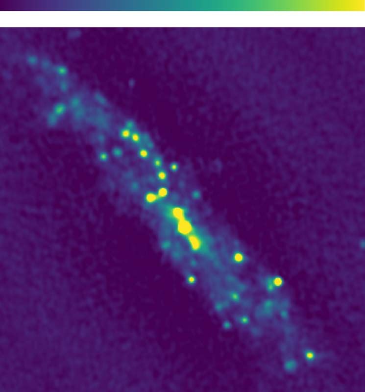
The Astrophysical Journal, 903:50 (24pp), 2020 November 1 Emig et al.
target in a campaign to characterize massive star clusters in image. Again, we use Briggs weighting with a robust parameter
local starbursts with ALMA. of r=0.5, which represents a good compromise between
The galaxy NGC4945 is unique in that it is one of the resolution and surface brightness sensitivity.
closest galaxies (3.8±0.3 Mpc; Karachentsev et al. 2007) After imaging, we convolved the continuum and line images
where a detected active galactic nucleus (AGN) and central to convert from an elliptical to a round beam shape. For the
starburst coexist. In the central ∼200 pc, the starburst full-bandwidth continuum image presented in this paper, the
dominates the infrared luminosity and ionizing radiation fiducial frequency is ν=93.2 GHz, and the final FWHM beam
(Marconi et al. 2000; Spoon et al. 2000 ), and an outflow of size is θ=0 12. The rms noise away from the source is
warm ionized gas has been observed (Heckman et al. 1990; ≈0.017 mJy beam−1, equivalent to 0.2 K in Rayleigh–Jeans
Moorwood et al. 1996; Mingozzi et al. 2019). Individual star brightness temperature units. Before convolution to a round
clusters have not previously been observed in NGC4945 due beam, the beam had a major and minor FWHM of
to the high extinction at visible and short IR wavelengths 0 097×0 071.
(e.g., AV36 mag; Spoon et al. 2000). Evidence for a For the H40α and H42α spectral cubes, the final FWHM
Seyfert AGN comes from strong, variable X-ray emission, as beam size is 0 20, convolved from 0 097×0 072 and
NGC4945 is one of the brightest sources in the X-ray sky and 0 11×0 083, respectively. The slightly lower resolution
has a Compton thick column density of 3.8×1024 cm−2 resulted in more sources with significantly detected line
(Marchesi et al. 2018). A kinematic analysis of H2O maser emission. We boxcar-smoothed the spectral cubes from the
emission yields a black hole mass of 1.4×10⁶ Me (Greenhill native 0.488 MHz channel width to 2.93 MHz. The typical rms
et al. 1997). in the H40α cube is 0.50 mJy beam−1 per 8.9 km s−1channel.
In this paper, we use ALMA to image the 93 GHz free–free The typical rms in the H42α cube is 0.48 mJy beam−1 per
continuum and hydrogen recombination line emission (H40α 10.3 km s−1channel.
and H42α) at 2.2 pc (0 12) resolution. This emission allows us As part of the analysis, we compare the high-resolution data
to probe photoionized gas on star cluster scales and thereby with observations taken in a 1 km intermediate configuration as
trace ionizing photon luminosities. We identify candidate star part of the same observing project. We use the intermediate-
clusters and estimate properties relating to their size, ionizing configuration data to trace the total recombination line emission
photon luminosity, stellar mass, and gas mass. of the starburst. We use the continuum image provided by the
Throughout this paper, we plot spectra in velocity units with observatory pipeline, which we convolve to have a circular
respect to a systemic velocity of Vsystematic=580 km s−1 in the beam FWHM of 0 7; the rms noise in the full-bandwidth
local standard of rest frame; estimates of the systemic velocity image is 0.15 mJy beam−1. The spectral cubes have a typical
vary by ±25 km s−1 (e.g., Chou et al. 2007; Roy et al. 2010; rms per channel of 0.24 mJy beam−1 with the same channel
Henkel et al. 2018). At a distance of 3.8 Mpc, 0 1 corresponds widths as the extended-configuration cubes. We do not jointly
to 1.84 pc. image the configurations because our main science goals are
focused on compact, pointlike objects. The extended-config-
uration data on their own are well suited to study these objects,
2. Observations
and any spatial filtering of extended emission will not affect the
We used the ALMA Band 3 receivers to observe NGC4945 analysis.
as part of the project 2018.1.01236.S (PI: A. Leroy). We We compare the continuum emission at 3 mm with archival
observed NGC4945 with the main 12 m array telescopes in ALMA imaging of the ν=350 GHz (λ∼850 μm) continuum
intermediate and extended configurations. Four spectral (project 2016.1.01135.S; PI: N. Nagar). At this frequency, dust
windows in Band 3—centered at 86.2, 88.4, 98.4, and emission dominates the continuum. We imaged the calibrated
100.1 GHz—capture the millimeter continuum primarily from visibilities with a Briggs robust parameter of r=−2 (toward
free–free emission and cover the hydrogen recombination lines uniform weighting), upweighting the extended baselines to
of principal quantum number (to the lower state) n = 40 and produce a higher-resolution image suitable for comparison to
42 from the α (Dn = 1) transitions. The rest frequency of our new Band 3 data. We then convolve the images to produce
H40α is 99.0230 GHz, and that of H42α is 85.6884 GHz. a circularized beam, resulting in an FWHM resolution of 0 12
In this paper, we focus on the 93 GHz (λ∼3.2 mm) (from an initial beam size of 0 10×0 064), exactly matched
continuum emission and the recombination line emission to our 93 GHz continuum image. These data have an rms noise
arising from compact sources in the starbursting region. We of 0.7 mJy beam−1 (0.2 K).
image the data from an 8 km extended configuration, which are We compare the ALMA data with Australian Long Baseline
sensitive to spatial scales of 0 07–6″ (2–100 pc), in order to Array (LBA) imaging of ν=2.3 GHz continuum emission
focus on the compact structures associated with candidate (Lenc & Tingay 2009). At this frequency and resolution, the
clusters. We analyze the observatory-provided calibrated radio continuum is predominantly synchrotron emission. We
visibilities using version 5.4.0 of the Common Astronomy use the Epoch 2 images (courtesy of E. Lenc) that have a native
Software Application (CASA; McMullin et al. 2007). angular resolution slightly higher than the 3 mm ALMA data,
When imaging the continuum, we flag channels with strong with a beam FWHM of 0 080×0 032 and an rms noise of
spectral lines. Then we create a continuum image using the full 0.082 mJy beam−1.
bandwidth of the line-free channels. We also make continuum
images for each spectral window. For all images, we use Briggs
3. Continuum Emission
weighting with a robust parameter of r=0.5.
When imaging the two spectral lines of interest, we first The whole disk of NGC4945, as traced by Spitzer IRAC
subtract the continuum in uv space through a first-order 8 μm emission (program 40410; PI: G. Rieke), is shown in
polynomial fit. Then, we image by applying a CLEAN mask Figure 1. The 8 μm emission predominantly arises from UV-
(to all channels) derived from the full-bandwidth continuum heated polycyclic aromatic hydrocarbons (PAHs), thus tracing
2
The Astrophysical Journal, 903:50 (24pp), 2020 November 1 Emig et al.
young and may still harbor reservoirs of gas, though in
Section 5.7, we find that the fraction of the mass still in gas
tends to be relatively small.
In Figure 3, the 93 GHz peaks without dust counterparts tend
to be strong sources of emission at 2.3 GHz (Lenc &
Tingay 2009), a frequency where synchrotron emission
typically dominates. As discussed in Lenc & Tingay (2009),
the sources at this frequency are predominantly supernova
remnants. The presence of 13 possible supernova remnants—
four of which are resolved into shell-like structures 1.1–2.1 pc
in diameter—indicates that a burst of star formation activity
started at least a few Myr ago. Lenc & Tingay (2009) modeled
the spectral energy distributions (SEDs) of the sources
spanning 2.3–23 GHz and found significant opacity at
2.3 GHz (τ=5–22), implying the presence of dense, free–
free plasma in the vicinity of the supernova remnants.
At 93 GHz, the very center of the starburst shows an elongated
region of enhanced emission (about 20 pc in projected length, or
∼1″) that is also bright in 350 GHz emission. This region is
connected to the areas of highest extinction. Higher column
Figure 1. Spitzer IRAC 8 μm emission from UV-heated PAHs over the full
densities of ionized plasma are also present in the region; Lenc &
galactic disk of NGC4945. The black square indicates the 8″×8″ Tingay’s (2009) observations reveal large free–free opacities, at
(150 pc×150 pc) central starburst region of interest in this paper; the inset least up to 23 GHz. The brightest peak at 93 GHz, centered at (α,
shows the ALMA 93 GHz continuum emission. δ)93=(13 h 05 m 27.4798 s±0.004 s, −49° 28′ 05.404″±
0.06″), is colocated with the kinematic center as determined from
H2O maser observations (a, d )H2 O =(13 h 05 m 27.279 s±
the interstellar medium and areas of active star formation. The 0.02s, −49° 28′ 04.44″±0.1″) (Greenhill et al. 1997) and
black square indicates the 8″×8″ (150 pc×150 pc) starburst presumably harbors the AGN core. We refer to the elongated
region that is of interest in this paper. region of enhanced emission surrounding the AGN core as the
Figure 2 shows the 93 GHz (λ∼3 mm) continuum emission circumnuclear disk. The morphological similarities between 93
in the central starburst of NGC4945. Our image reveals and 350 GHz, together with the detection of a synchrotron point
∼30 peaks of compact, localized emission with peak flux source (likely a supernova remnant; see Section 3.2 and source
densities of 0.6–8 mJy (see Section 3.1). On average, the 17) in the circumnuclear disk, indicate that star formation is likely
continuum emission from NGC4945 at this frequency is present there.
dominated by thermal, free–free (bremsstrahlung) radiation
(Bendo et al. 2016). Free–free emission from bright, compact
3.1. Point-source Identification
regions may trace photoionized gas in the immediate
surroundings of massive stars. We take into consideration the We identify candidate star clusters via pointlike sources of
pointlike sources detected at 93 GHz as candidate massive star emission in the 93 GHz continuum image. Sources are found
clusters, though some contamination by synchrotron-domi- using PyBDSF (Mohan & Rafferty 2015) in the following way.
nated supernova remnants or dusty protoclusters may still be Islands are defined as contiguous pixels (of nine pixels or
possible. The morphology of the 93 GHz emission and more) above a threshold of seven times the global rms value of
clustering of the peaks indicate possible ridges of star σ≈0.017 mJy beam−1. Within each island, multiple Gaus-
formation and shells. The extended, faint negative bowls sians may be fit, each with a peak amplitude greater than the
flanking the main disk likely reflect the short spacing data peak threshold of 10 times the global rms. We chose this peak
missing from this image. We do not expect that they affect our threshold to ensure that significant emission can also be
analysis of the point source–like cluster candidates. identified in the continuum images made from individual
The large amount of extinction present in this high- spectral windows. The number of Gaussians is determined
inclination central region (i∼72°; Henkel et al. 2018) has from the number of distinct peaks of emission higher than the
previously impeded the direct observation of its star clusters. peak threshold that have a negative gradient in all eight
The Paschen-α (Paα) emission (Marconi et al. 2000) of the evaluated directions. Starting with the brightest peak, Gaus-
n = 3 hydrogen recombination line at 1.87 μm, shown in sians are fit and cleaned (i.e., subtracted). A source is identified
Figure 3, reveals faint emission above and below the star- with a Gaussian as long as subtracting its fit does not increase
forming plane. Corrected for extinction, the clumps of ionized the island rms.
emission traced by Paα would give rise to free–free emission Applying this algorithm to our 93 GHz image yielded 50
below our ALMA detection limit. The Paα and mid-infrared Gaussian sources. We remove five sources that fall outside of
(MIR) spectral lines give support for dust extinction of the star-forming region. We also remove three sources that
AV>160 mag surrounding the AGN core and more generally appeared blended, with an offset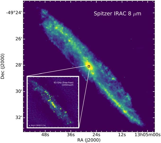
The Astrophysical Journal, 903:50 (24pp), 2020 November 1 Emig et al.
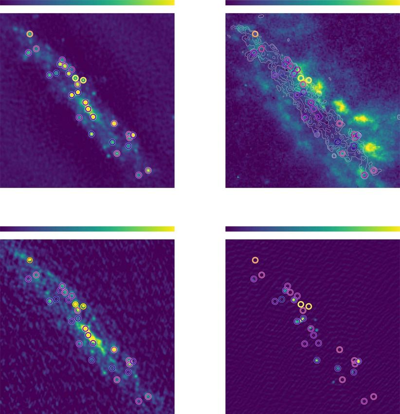
Figure 2. ALMA 93 GHz (λ∼3.2 mm) continuum emission in the central starburst of NGC4945. The continuum at this frequency is dominated by ionized, free–
free emitting plasma. In this paper, we show that the pointlike sources are primarily candidate massive star clusters. The brightest point source of emission at the center
is presumably the Seyfert AGN. The rms noise away from the source is σ≈0.017 mJy beam−1, and the circularized beam FWHM is 0 12 (or 2.2 pc at the distance of
NGC4945). The contours of the continuum image show 3σemission (gray) and [4σ, 8σ, 16σ, K256σ] emission (black).
with the apertures used for flux extraction. The sources match (source 18), which, due to self-absorption at frequencies greater
well with what we would identify by eye. than 23 GHz, is bright at 93 GHz but not at 2.3 GHz and
therefore has the lowest S2.3/S93 ratio.
3.2. Point-source Flux Extraction From the continuum measurements, we construct simple
SEDs for each source. These SEDs are used for illustrative
For each source, we extract the continuum flux density at purposes and do not affect the analysis in this paper. Examples
2.3, 93, and 350 GHz through aperture photometry. Before of the SEDs of three sources are included in Figure 5. We show
extracting the continuum flux at 2.3 GHz, we convolve the an example of a free–free-dominated source (source 22), which
image to the common resolution of 0 12. We extract the flux represents the majority of sources, as well as a dust- (source 12)
density at the location of the peak source within an aperture and a synchrotron- (source 14) dominated source. Of the
diameter of 0 24. Then we subtract the extended background sources with extracted emission of >3σ at 2.3 GHz, nine also
continuum that is local to the source by taking the median flux have the free–free absorption of their synchrotron spectrum
density within an annulus of inner diameter 0 24 and outer modeled. We plot this information whenever possible. When a
diameter 0 30; using the median suppresses the influence of source identified by Lenc & Tingay (2009) lies within 0 06
nearby peaks and the bright surrounding filamentary features. (half the beam FWHM) of the 93 GHz source, we associate the
The flux density of each source at each frequency is listed in low-frequency modeling with the 93 GHz source. We take the
Table 1. When the extracted flux density within an aperture is model fit by Lenc & Tingay (2009) and normalize it to the
less than three times the global rms noise (in the 2.3 and 2.3 GHz flux that we extract; as an example, see the solid
350 GHz images), we assign a 3σ upper limit to that flux purple curve in the middle panel of Figure 5. The SEDs of all
measurement. sources are shown in Figure 13 in Appendix C.
In Figure 4, we plot the ratio of the flux densities extracted at
350 and 93 GHz (S350/S93) against the ratio of the flux
densities extracted at 2.3 and 93 GHz (S2.3/S93). Synchrotron-
3.3. Free–Free Fraction at 93 GHz
dominated sources, which fall to the bottom right of the plot,
separate from the free–free- (and dust-) dominated sources, The flux density of optically thin, free–free emission at
which lie in the middle of the plot. One exception is the AGN millimeter wavelengths (see Appendix A.2; Draine 2011)
4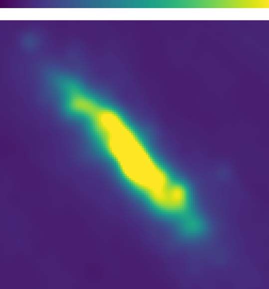
The Astrophysical Journal, 903:50 (24pp), 2020 November 1 Emig et al.
Figure 3. Top left: 93 GHz continuum emission with sources identified; also see Table 1. Circles show apertures (diameter of 0 24) used for continuum extraction.
Their colors indicate the measured in-band spectral index, as in Figure 4, where dark purple indicates synchrotron-dominated emission and yellow indicates dust-
dominated emission. Top right: HST Paα emission–hydrogen recombination line, n = 3, at 1.87 μm (courtesy of P. van der Werf) tracing ionized gas at ≈0 2
resolution (Marconi et al. 2000). Dust extinction of AV>36 mag obscures the Paα recombination emission at shorter wavelengths from the starburst region. Contours
trace 93 GHz continuum, as described in Figure 2. Bottom left: ALMA 350 GHz continuum emission tracing dust. Bottom right: Australian LBA 2.3 GHz continuum
imaging of synchrotron emission primarily from supernova remnants (Lenc & Tingay 2009).
arises as where EMC=nen+V is the volumetric emission measure of the
ionized gas, D is the distance to the source, and Te is the
⎛ n e n +V ⎞ electron temperature of the medium. Properties of massive star
Sff = (2.08 mJy) ⎜ ⎟
⎝ 5 ´ 108 cm-6 pc3 ⎠ clusters (i.e., ionizing photon rate) can thus be derived through
-2 an accurate measurement of the free–free flux density and an
⎛ Te ⎞-0.32 ⎛ n ⎞-0.12 ⎛ D ⎞
´ ⎜ ⎟ ⎜ ⎟ ⎜ ⎟ , (1 ) inference of the volumetric emission measure. We will
⎝ 10 4 K ⎠ ⎝ 100 GHz ⎠ ⎝ 3.8 Mpc ⎠ determine a free–free fraction, fff, and let Sff=fffS93.
5The Astrophysical Journal, 903:50 (24pp), 2020 November 1 Emig et al.
Table 1
Properties of the Continuum Emission from Candidate Star Clusters
Source R.A. Decl. S93 α93 S2.3a S350b fff fsync fdc
(mJy) (mJy) (mJy)
1 13:05:27.761 −49:28:02.83 1.28±0.13 −0.80±0.11 2.3±0.4 L 0.51±0.08 0.49 L
2 13:05:27.755 −49:28:01.97 1.01±0.10 0.80±0.22 L 26.6 0.78±0.05 L 0.22
3 13:05:27.724 −49:28:02.64 0.82±0.08 −0.27±0.23 L 14.8 0.89±0.16 0.11 L
4 13:05:27.662 −49:28:03.85 0.95±0.09 −1.12±0.42 L 16.0 0.27±0.31 0.73 L
5 13:05:27.630 −49:28:03.76 0.77±0.08 −1.57±0.63 L L 0.00±0.40 1.00 L
6 13:05:27.612 −49:28:03.35 1.73±0.17 −1.11±0.22 7.1±0.7 L 0.28±0.16 0.72 L
7 13:05:27.602 −49:28:03.15 0.98±0.10 −0.61±0.19 L 15.5 0.65±0.14 0.35 L
8 13:05:27.590 −49:28:03.44 1.89±0.19 −0.40±0.20 L 14.9 0.80±0.15 0.20 L
9 13:05:27.571 −49:28:03.78 1.76±0.18 −1.01±0.22 12.2±1.2 L 0.36±0.16 0.64 L
10 13:05:27.558 −49:28:04.77 2.41±0.24 −1.10±0.20 9.5±0.9 L 0.29±0.14 0.71 L
11 13:05:27.557 −49:28:03.60 0.76±0.08 −0.59±0.38 L 13.9 0.66±0.28 0.34 L
12 13:05:27.540 −49:28:03.99 1.28±0.13 1.47±0.37 L 37.4 0.62±0.09 L 0.38
13 13:05:27.530 −49:28:04.27 1.78±0.18 −0.22±0.15 L 20.8 0.93±0.11 0.07 L
14 13:05:27.528 −49:28:04.63 3.06±0.31 −1.22±0.19 14.3±1.4 11.2 0.20±0.14 0.80 L
15 13:05:27.522 −49:28:05.80 0.83±0.08 −0.71±0.28 L L 0.57±0.21 0.42 L
16 13:05:27.503 −49:28:04.08 0.98±0.10 1.34±0.37 L 23.9 0.65±0.09 L 0.35
17 13:05:27.493 −49:28:05.10 3.69±0.37 −0.61±0.13 5.3±0.5 47.1 0.65±0.10 0.35 L
18 13:05:27.480 −49:28:05.40 9.74±0.97 −0.85±0.05 L 39.0 0.47±0.03 0.53 L
19 13:05:27.464 −49:28:06.55 1.30±0.13 −1.36±0.38 7.8±0.8 L 0.10±0.28 0.90 L
20 13:05:27.457 −49:28:05.76 2.51±0.25 −0.88±0.13 L 22.4 0.45±0.09 0.55 L
21 13:05:27.366 −49:28:06.92 1.19±0.12 −1.38±0.41 4.7±0.5 L 0.09±0.30 0.91 L
22 13:05:27.358 −49:28:06.07 2.57±0.26 −0.19±0.18 L 34.8 0.95±0.13 0.05 L
23 13:05:27.345 −49:28:07.44 0.95±0.09 −0.28±0.25 L 9.7 0.88±0.18 0.12 L
24 13:05:27.291 −49:28:07.10 0.90±0.09 −1.22±0.36 3.2±0.4 L 0.20±0.26 0.80 L
25 13:05:27.288 −49:28:06.56 0.91±0.09 −0.27±0.35 2.1±0.4 15.2 0.89±0.26 0.11 L
26 13:05:27.285 −49:28:06.72 1.13±0.11 −0.33±0.38 1.4±0.4 18.5 0.85±0.28 0.15 L
27 13:05:27.269 −49:28:06.60 2.75±0.28 −1.08±0.14 31.2±3.1 L 0.30±0.10 0.70 L
28 13:05:27.242 −49:28:08.43 0.80±0.08 −0.54±0.12 L L 0.70±0.09 0.30 L
29 13:05:27.198 −49:28:08.22 1.43±0.14 −0.29±0.20 L 12.6 0.88±0.14 0.12 L
Notes.Here R.A. and decl. refer to the center location of a Gaussian source identified in the 93 GHz continuum image in units of hour angle and degrees, respectively;
S93 is the flux density in the 93 GHz full-bandwidth continuum image; α93 is the spectral index at 93 GHz (S∝ν α), as determined from the best-fit slope to the
85–101 GHz continuum emission; S2.3 is the flux density extracted in the 2.3 GHz continuum image; S350 is the flux density extracted in the 350 GHz continuum
image; and fff, fsyn, and fd are the free–free, synchrotron, and dust fractional contribution to the 93 GHz continuum emission, respectively, as determined from the
spectral index. See Section 3.3 for a description of how the errors on these fractional estimates are determined.
a
A 3σ upper limit to the sources undetected in 2.3 GHz continuum emission is 1.2 mJy.
b
The error on the 350 GHz flux density measurement is 3.2 mJy. A 3σ upper limit to the undetected sources is 9.6 mJy.
c
The error on the fractional contributions is the same as for fff unless otherwise noted.
In this section, we focus on determining the portion of free– spectral window using aperture photometry with the same
free emission that is present in the candidate star clusters at aperture sizes as described in Section 3.2. We fit a first-order
93 GHz. To do this, we need to estimate and remove polynomial to the five continuum measurements—four from
contributions from synchrotron emission and dust continuum. each spectral window and one from the full-bandwidth image.
We determine an in-band spectral index across the 15 GHz The fit to the in-band spectral index is listed in Table 1 with the
bandwidth of the ALMA Band 3 observations. Using the 1σ uncertainty to the fit. The median uncertainty of the spectral
spectral index,12 we constrain the free–free fraction, as well as indices is 0.13. The spectral indices measured in this way were
the fractional contributions of synchrotron and dust (see consistent for the brightest sources with the index determined
Figure 4 and Table 1). We found the in-band index to give by CASA tclean; however, we found our method to be more
stronger constraints and, for 2.3 GHz, be more reliable than reliable for the fainter sources. Nonetheless, the errors are large
extrapolating (assuming indices of −0.8, −1.5) because of the for faint sources.
two decades’ difference in frequency coupled with the large
optical depths already present at 2.3 GHz.
3.3.2. Decomposing the Fractional Contributions of Emission Type
3.3.1. Band 3 Spectral Index
From the in-band spectral index fit, we estimate the
We estimate an in-band spectral index at 93 GHz, α93, from fractional contribution of each emission mechanism—free–
a fit to the flux densities in the spectral window continuum free, synchrotron, and (thermal) dust—to the 93 GHz con-
images of the ALMA Band 3 data. The spectral windows span tinuum. To do this, we simulate how mixtures of synchrotron,
15 GHz, which we set up to have a large fractional bandwidth. free–free, and dust emission could combine to create the
We extract the continuum flux density of each source in each observed in-band index. We assume fixed spectral indices for
each component and adjust their fractions to reproduce the
12
Similar methods have been used by, e.g., Linden et al. (2020). observations (see below).
6The Astrophysical Journal, 903:50 (24pp), 2020 November 1 Emig et al.
Figure 4. Top:ratio of the flux densities extracted at 350 and 93 GHz
(S350/S93) plotted against the ratio of the flux densities extracted at 2.3 and
93 GHz (S2.3/S93). Bottom: the relation we use to determine the free–free
fraction from the in-band index, α93, at 93 GHz. Data points in both plots are
colored by the in-band index derived only from our ALMA data. Yellow
indicates dust-dominated sources, whereas purple indicates synchrotron-
dominated sources. Candidate star clusters in which free–free emission
dominates at 93 GHz appear ∼pink. The diameter of each data point is Figure 5. Example SEDs constructed for each source. Top: dust-dominated,
proportional to the flux density at 93 GHz and correspondingly inversely source 12. Middle: synchrotron-dominated, source 14. Bottom: free–free-
proportional to the error of the in-band spectral index. dominated, source 22. The dashed orange line represents a dust spectral index
of α=4.0, normalized to the flux density we extract at 350 GHz (orange data
We consider that a source is dominated by two types of point). The dashed black line represents a free–free spectral index of
α=−0.12, normalized to the flux density we extract at 93 GHz (black data
emission (a caveat we discuss in detail in Section 6): free–free point). The pink data points show the flux densities extracted from the Band 3
and dust or free–free and synchrotron. With synthetic data spectral windows. The gray shaded region is the 1σ error range of the Band 3
points, we first set the flux density at 93 GHz, S93, to a fixed spectral index fit, except we have extended the fit in frequency for displaying
value and vary the contributions of dust and free–free continua, purposes. The purple line represents a synchrotron spectral index of α=−1.5,
normalized to the flux density we extract at 2.3 GHz (purple data point), except
such that S93=Sd+Sff. For each model, we determine the for source 14, where the solid purple line represents the normalized
continuum flux at each frequency across the Band 3 frequency 2.3–23 GHz fit from Lenc & Tingay (2009). Error bars on the flux density
coverage as the sum of the two components. We assume that data points are 3σ.
the frequency dependence of the free–free component is
αff=−0.12 and the frequency dependence of the dust
component is αd=4.0. We fit the (noiseless) continuum of free–free fraction of the candidate star clusters when the fit to
the synthetic data across the Band 3 frequency coverage with a their in-band index is α93−0.12.
power law, determining the slope as α93, the in-band index. We Our choices for the spectral indices of the three emission
express the results in terms of free–free and dust fractions, types are motivated as follows. In letting αff=−0.12, we
rather than absolute flux. In this respect, we explore free–free assume that the free–free emission is optically thin (e.g., see
fractions to the 93 GHz continuum ranging from fff=(0.001, Appendix A.2). We do not expect significant free–free opacity
0.999) in steps of 0.001. We let the results of this process at 93 GHz given the somewhat-evolved age of the candidate
constrain our free–free fraction when the in-band index clusters in the starburst (see Section 5.2). In letting αd=4.0,
measured in the actual (observed) data is α93 −0.12. we assume the dust emission is optically thin with a
Next, we repeat the exercise, but we let synchrotron and wavelength-dependent emissivity so that τ∝λ−2 (e.g., see
free–free dominate the contribution to the continuum at Draine 2011). The low dust optical depths estimated in
93 GHz. We take the frequency dependence of the free–free Section 5.6 imply a dust spectral index steeper than 2, though
component as αff=−0.12 across the Band 3 frequency the exact value might not be 4, e.g., if our assumed emissivity
coverage, and we set the synchrotron component to power-law index is not applicable. The generally faint dust
αsyn=−1.5. We let the results of this process constrain the emission indicates that our assumptions about dust do not have
7The Astrophysical Journal, 903:50 (24pp), 2020 November 1 Emig et al.
a large effect on our results. For the synchrotron frequency where bn + 1 is the local thermodynamic equilibrium (LTE)
dependence, we assume αsyn=−1.5. This value is consistent departure coefficient, EML=nenpV is the volumetric emission
with the best-fit slope of αsyn=−1.4 found by Bendo et al. measure of ionized hydrogen, D is the distance to the source, Te
(2016) averaged over the central 30″ of NGC4945. Further- is the electron temperature of the ionized gas, and ν is the rest
more, the median slope of synchrotron-dominated sources frequency of the spectral line.
modeled at 2.3–23 GHz is −1.11 (Lenc & Tingay 2009), Figure 6 shows the spectra of the 15 sources with detected
indicating that even at 23 GHz, the synchrotron spectra already radio recombination line emission. We extract H40α and H42α
show losses due to aging, i.e., are steeper than a canonical spectra at the location of each source with an aperture diameter
initial injection of αsyn≈−0.8. While our assumed value of of 0 4, or twice the beam FWHM. We average the spectra of
αsyn=−1.5 is well motivated, on average, variations from the two transitions together to enhance the signal-to-noise ratio
source to source are likely present. of the recombination line emission. To synthesize an effective
Through this method of decomposition, the approximate H41α profile, we interpolate the two spectra of each source to a
relation between the in-band index and the free–free fraction is fixed velocity grid with a channel width of 10.3 km s−1; weight
⎧ 0.72 a 93 + 1.09, - 1.5 a 93 - 0.12 each spectrum by s-rms 2
, where σrms is the spectrum standard
fff = ⎨ , (2 ) deviation; and average the spectra together, lowering the final
⎩- 0.24 a 93 + 0.97, 4.0 a 93 - 0.12 noise. The averaged spectrum has an effective transition of
H41α at νeff=92.034 GHz.
for which α93−0.12, the synchrotron fraction is found to be We fit spectral features with a Gaussian profile. We calculate
fsyn=1 − fff and we set fd=0, and for which α93 −0.12 an integrated signal-to-noise ratio for each line by integrating
the dust fraction is found to be fd=1 − fff and fsyn=0. This the spectrum across the Gaussian width of the fit (i.e., ±σGaus)
relation is depicted in the bottom panel of Figure 4 using the and then dividing by the noise over the same region, N srms,
values that have been determined for each source. where N is the number of channels covered by the region. We
report on detections with an integrated signal of >5σrms.
3.3.3. Estimated Free–Free, Synchrotron, and Dust Fractions to the Table 2 summarizes the properties of the line profiles derived
93 GHz Continuum from the best-fit Gaussian. The median rms of the spectra is
σrms=0.34 mJy.
Table 1 and Figure 4 summarize our estimated fractional In Figure 12 of Appendix B, we show that the central
contribution of each emission mechanism to the 93 GHz velocities of our detected recombination lines are in good
continuum of each source. We use the same relation above to agreement with the kinematic velocity expected of the disk
translate the range of uncertainty on the spectral index to an rotation. To do this, we overlay our spectra on H40α spectra
uncertainty in the emission fraction estimates. We find that, at extracted from the intermediate-configuration observations
this 0 12 resolution, the median free–free fraction of sources is (0 7 resolution).
fff=0.62, with a median absolute deviation of 0.29. Most of In 12 of the 15 sources, we detect relatively narrow features
the spectral indices are negative, and as a result, we find that of FWHM∼(24–58) km s−1. Larger line widths of
synchrotron emission can have a nontrivial contribution with a FWHM∼(105–163) km s−1 are observed from bright sources
median fraction of fsyn=0.36 and median absolute deviation that also have high synchrotron fractions, indicating that
of 0.32. On the other hand, three of the measured spectral multiple components, unresolved motions (e.g., from expand-
indices are positive. The median dust fraction of sources is ing shells or galactic rotation), or additional turbulence may be
fd=0 with a median absolute deviation of 0.10. A 1σlimit on present. Six sources with detected recombination line emission
the fractional contribution of dust does not exceed fd=0.47 have considerable ( fsyn0.50) synchrotron emission (i.e.,
for any single source. sources 1, 4, 6, 14, 21, and 27) at 93 GHz.
Additional continuum observations of comparable resolution In the top panel of Figure 7, we show the total recombination
at frequencies between 2 and 350 GHz would improve the line emission extracted from the starburst region in the 0 2
estimates of the fractional contribution of free–free, dust, and resolution “extended” configuration observations. The aperture
synchrotron to the 93 GHz emission. we use, designated as region T1, is shown in Figure 8. Details
of the aperture selection are described in Section 4.1.1. The
4. Recombination Line Emission spectrum consists of two peaks reminiscent of a double horn
Hydrogen recombination lines at these frequencies trace profile representing a rotating ring. We fit the spectrum using
ionizing radiation (E>13.6 eV); this recombination line the sum of two Gaussian components. In Table 3, we include
emission is unaffected by dust extinction. The integrated the properties of the best-fit line profiles. The sum total area of
emission from a radio recombination line transition to quantum the fits is (2.1±0.6)Jy km s−1.
number n, which we derive for millimeter-wavelength transi-
tions in Appendix A.1, is described by
4.1. Line Emission from 0 7 Resolution, Intermediate-
ò Sn dv = (65.13 mJy km s-1) configuration Observations
Figure 7 also shows integrated spectra derived from
⎛ ne np V ⎞ ⎛ D ⎞-2
´ bn + 1⎜ ⎟⎜ ⎟ intermediate-resolution (0 7) data. We use these data as a
⎝ 5 ´ 108 cm-6 pc3 ⎠ ⎝ 3.8 Mpc ⎠ tracer of the total ionizing photons of the starburst region. We
expect that the intermediate-resolution data include emission
⎛ Te ⎞-1.5 ⎛ n ⎞
´ ⎜ ⎟ ⎜ ⎟, (3 ) from both discrete, pointlike sources and diffuse emission from
⎝ 10 4 K ⎠ ⎝ 100 GHz ⎠ any smooth component.
8The Astrophysical Journal, 903:50 (24pp), 2020 November 1 Emig et al.
Figure 6. Radio recombination line spectra for sources with significantly detected emission. The thin blue line is the H40α spectrum. The thin green line is the H42α
spectrum. These spectra have been regridded from their native velocity resolution to the common resolution of 10.3 km s−1. The thick black line is the weighted
average spectrum of H40α and H42α, effectively H41α. In red is the best fit to the effective H41α radio recombination line feature.
The total integrated emission in the intermediate-configura- 4.1.1. Total Emission from the Starburst Region
tion data is about three times larger than the integrated emission In Figure 8, we show the integrated intensity map of H40α
in the extended-configuration data. Spectra representing the emission integrated in vsystemic±170 km s−1 as calculated
total integrated line flux are shown in Figure 7. In Figure 8, we from the 0 7 intermediate-configuration data. Diffuse emission
show the integrated intensity map of H40α emission from the is detected throughout the starburst region and up to 30 pc in
intermediate-configuration (0 7) data. In Table 3, we include apparent size beyond the region where we detect the bright
the best-fit line profiles. point sources at high resolution.
We also compare the line profiles of H40α and H42α in Also shown in Figure 8 are the apertures used to extract
the intermediate-configuration (0 7) data; see Table 4 spectra in Figure 7. We fit a two-dimensional Gaussian to the
and Figures 9and 10. We find that the integrated line continuum emission in the 0 7 resolution observations (see
emission of H42α is enhanced compared with H40α, Figure 9). This results in a best fit centered at (α,
reaching a factor of 2 greater when integrated over the entire δ)=(13hr 05m 27 4896, −49° 28′ 05 159), with major and
starburst region. Yet we see good agreement between the two minor Gaussian widths of σmaj=2 4 and σmin=0 58 and an
lines at the scale of individual cluster candidates. Spectral angle of θ=49°. 5; we use this fit as a template for the aperture
lines (possibly arising from c-C3H2) likely contaminate the location, position angle, width, and height. We independently
H42α line flux in broad, typically spatially unresolved line vary the major and minor axes (in multiples of 0.5σmaj and
profiles. 0.5σmin, respectively) in order to determine the aperture that
9The Astrophysical Journal, 903:50 (24pp), 2020 November 1 Emig et al.
Figure 8. Integrated intensity (moment 0) map of H40α emission integrated at
Vsystemic±170 km s−1 and observed with the intermediate telescope
configuration at native 0 7 resolution. Overlaid are contours of the 93 GHz
Figure 7. The H40α line spectra extracted from the aperture regions T1 (top)
continuum from extended-configuration, high-resolution (0 12) data as
and T2 (bottom; see Figure 8). In blue is the extended-configuration
described in Figure 1. Red ellipses mark the apertures used to extract the
(“extended”) spectrum extracted from the high-resolution 0 2 data; this
total line emission from regions T1 and T2.
spectrum shows the maximum total integrated line flux extracted. In purple is
the intermediate-configuration (“intermed”) spectra extracted from low-
resolution, native 0 7 data; the spectrum from the T2 region is the total
maximum integrated line flux from these data. The solid black line represents
the sum total of two Gaussian fits. The dotted black line represents the single
Gaussian fits.
Table 2
Average Line Profiles Nominally Located Near H41α
Source Vcen Peak FWHM σrms
(km s−1) (mJy) (km s−1) (mJy)
1 131.6±12 0.69±0.16 105.2±28 0.35
3 117.4±4.0 1.26±0.28 37.2±9.4 0.36
4 107.5±4.3 1.28±0.26 42.9±10 0.36
6 79.4±3.1 1.33±0.27 31.1±7.3 0.33
7 77.2±3.0 1.46±0.32 28.1±7.0 0.36
8 87.5±2.1 2.24±0.24 38.7±4.9 0.33
12 53.6±3.9 1.72±0.24 55.9±9.1 0.39
13 45.7±1.7 2.68±0.26 34.8±3.9 0.31
14 111.8±12 0.82±0.12 163.1±28 0.33
15 5.6±2.8 1.62±0.33 28.2±6.6 0.37
21 −140.7±8.3 0.99±0.15 113.3±20 0.34
22 −80.6±4.0 1.61±0.22 58.4±9.4 0.34
25 −102.3±3.3 1.42±0.24 39.0±7.7 0.32
26 −107.6±2.2 1.86±0.27 30.9±5.3 0.33
27 −102.3±1.6 2.02±0.27 23.6±3.6 0.28
Note.Here Vcen is the central velocity of the best-fit Gaussian, peak is the peak Figure 9. Continuum emission at 93 GHz observed with an intermediate
configuration with native resolution FWHM=0 7 (or 12.9 pc at the distance
amplitude of the Gaussian fit, FWHM is the FWHM of the Gaussian fit, and
of NGC4945). The rms noise away from the source is σ≈0.15 mJy beam−1.
σrms is the standard deviation of the fit-subtracted spectrum. The contours of the continuum image show 3σemission (gray) and [4σ, 8σ,
16σ, K] emission (black). Apertures (red) with a diameter of 4″ mark the
maximizes the total integrated signal in channels within regions N, C, and S.
±170 km s−1. With the extended-configuration cube, we find
the largest integrated line emission with an aperture of We extract the total H40α line flux from the intermediate-
8 4×1 5, which we refer to as T1. With the intermediate- configuration (0 7 resolution) cube using the T2 aperture (see
configuration cube, the largest integrated line emission arises bottom panel of Figure 7). The spectrum shows a double horn
with an aperture of 12 0×2 9, which we refer to as T2. profile, indicating ordered disklike rotation. We fit the features
10The Astrophysical Journal, 903:50 (24pp), 2020 November 1 Emig et al.
Table 3
H40α Line Profiles from the Regions of Total Flux
Region Config. Vcen,1 Peak1 FWHM1 Vcen,2 Peak2 FWHM2 H40α Flux
(km s−1) (mJy) (km s−1) (km s−1) (mJy) (km s−1) (mJy km s−1)
T1 Extended −139±9 9.7±2 78±22 91±13 8.9±1.8 138±14 2100±600
T1 Intermed −117±9 16±3 99±21 66±2 16±2 186±15 4800±900
T2 Intermed −114±13 19±4 113±31 86±13 23±3 167±14 6400±1000
Table 4
Comparison of Integrated Recombination Line Flux
Region H42α Flux H40α Flux Ratio H42α/H40α
(Jy km s−1) (Jy km s−1)
N 2.1±0.2 1.5±0.2 1.4±0.2
C 5.9±0.3 3.7±0.3 1.6±0.2
S 1.9±0.2 0.96±0.1 2.0±0.3
with two Gaussians. The sum total of their integrated line flux
is (6.4±1.0)Jy km s−1.
We also extract H40α line flux from the intermediate-
configuration (0 7 resolution) cube within the T1 aperture in
order to directly compare the integrated line flux in the two
different data sets using the same aperture regions. We find
more emission in the intermediate-configuration data, a factor
of ∼2.3 greater than the extended-configuration data. This
indicates that some recombination line emission originates on
large scales (>100 pc) to which the high-resolution long
baselines are not sensitive.
4.1.2. H42α Contamination
In this section, we compare the line profiles from H40α and
H42α extracted from the 0 7 intermediate-configuration data.
In principle, we expect the spectra to be virtually identical,
which is why we average them to improve the signal-to-noise
ratio at high resolution. Here we test that assumption at low
resolution. To summarize, we find evidence that a spectral line
may contaminate the H42α measured line flux in broad
(typically spatially unresolved) line profiles. Yet we see good
agreement between the two lines at the scale of individual
cluster candidates.
We extracted spectra in three apertures to demonstrate the
constant velocity offset of the contaminants. We approximately
matched the locations of these apertures to those defined in
Bendo et al. (2016), in which H42α was analyzed at 2 3 Figure 10. Comparison of our H40α (purple) and H42α (green) from
resolution; in this way, we are able to confirm the flux and line intermediate-configuration, low-resolution data from the regions defined in
profiles we extract at 0 7 resolution with those at 2 3. The Figure 9 as N (top), C (middle), and S (bottom). We find H42α to be
nonoverlapping circular apertures with diameters of 4″ contaminated by spectral lines that may include c-C3H2 432−423, shown as a
dashed line in the panels at expected velocities with respect to H42α. When
designated as north (N), center (C), and south (S) are shown in contaminant lines are included, the integrated line flux of H42α is
Figure 9. overestimated by a factor of 1.5 in these apertures; this grows to a factor of
We used our intermediate-configuration data to extract an 2 when integrating over the total starburst emission.
H40α and H42α spectrum in each of the regions. We overplot
the spectra of each region in Figure 10. We fit a single indicates that we are recovering the H42α total line flux and
Gaussian profile to the line emission, except for the H42α properties with our data.
emission in region N, where two Gaussian components better On the other hand, the H40α flux we extract is about a factor
minimized the fit. The total area of the fits is presented in of ∼1.6 lower than the H42α fluxes in these apertures (see
Table 4 as the integrated line flux. Figure 10 and Table 4). The discrepancy grows to a factor of 2
Our line profiles of H42α are similar in shape and velocity in the profile extracted from the total region.
structure to those analyzed in Bendo et al. (2016), and the The additional emission seen in the H42α spectrum at
integrated line emission is also consistent (within 2σ). This velocities of +100 to +250 km s−1 with respect to the bright,
11The Astrophysical Journal, 903:50 (24pp), 2020 November 1 Emig et al.
Table 5
Temperature Analysis
Source ò SL dV S93 fff Te
(mJy km s−1) (mJy) (K)
8 92±15 3.5±0.4 0.74±0.20 6000±1700
13 99±14 2.9±0.3 0.91±0.22 5600±1400
22 100±21 3.4±0.3 0.78±0.20 5600±1700
26 61±13 2.6±0.3 0.72±0.29 6400±2600
27 50±10 3.6±0.4 0.45±0.16 6500±2300
Note.Here ò SL dV refers to the integrated line emission, S93 is the continuum
flux density extracted at 93 GHz in the 0 2 resolution image, fff is the
estimated free–free fraction at 0 2 resolution, and Te is the electron
temperature derived using Equation (4).
presumably hydrogen recombination line peak is absent in the
H40α profile. It is not likely to be a maser-like component of
hydrogen recombination emission, since the relative flux does
not greatly vary in different extraction regions, and densities
outside of the circumnuclear disk would not approach the
emission measures necessary (e.g., EMv1010 cm−6 pc3) for
stimulated line emission.
We searched for spectral lines in the frequency range
νrest∼85.617–85.660 GHz corresponding to these velocities
and find several plausible candidates, though we were not able Figure 11. Top:complementary cumulative distribution of the ionizing photon
to confirm any species with additional transitions in the rate, Q0, of candidate star clusters in NGC4945 (see Table 6) and NGC253
(E.A.C. Mills et al. 2020, in preparation). The turnoff at lower values likely
frequency coverage of these observations. A likely candidate reflects completeness limits. Bottom: stellar mass, Må, of our candidate star
may be the 432−423 transition of c-C3H2. This molecule has a clusters inferred from the ionizing photon rates of a cluster with an age of 5 Myr,
widespread presence in the diffuse interstellar medium (ISM) plotted as a complementary cumulative distribution. We also include the stellar
of the Galaxy (e.g., Lucas & Liszt 2000), and the 220−211 masses of clusters in the starburst of NGC253 (E.A.C. Mills et al. 2020, in
preparation) and the galaxies LMC, M51, and the Antennae (Mok et al. 2020).
transition has been detected in NGC4945 (Eisner et al. 2019). Since the clusters in NGC253 are likely close to a zero-age main sequence, they
As an example, we plot the velocity of c-C3H2 432−423 would produce more ionizing photons per unit mass as compared with the
relative to H42α in Figure 10. slightly older stellar population in the clusters of NGC4945.
5. Physical Properties of the Candidate Star Clusters 2.2 pc. The uncertainties we report reflect the errors of the
In this section, we estimate the properties of the candidate Gaussian fit.
star clusters, summarized in Table 6. We discuss their size and Based on high-resolution imaging of embedded clusters in
approximate age. Properties of the ionized gas content, such as the nucleus of the Milky Way and NGC253, some of these
temperature (see Table 5), metallicity, density, and mass, are clusters might break apart at higher resolution (Ginsburg et al.
derived from the continuum and recombination line emission. 2018, Levy et al., in preparation). If they follow the same
We estimate the ionizing photon rate of the candidate star pattern seen in these other galaxies, each source would have
clusters and use it to infer the stellar mass (see Figure 11). one or two main components with potentially several
From the dust emission at 350 GHz, we estimate the gas masses associated fainter components.
of the candidate star clusters. With a combined total mass from
gas and stars, we estimate current mass surface densities and 5.2. Age
freefall times. Throughout our analysis, we assume that the candidate star
We exclude source 5 from the analysis, since the free–free clusters formed in an instantaneous burst of star formation
fraction is fffThe Astrophysical Journal, 903:50 (24pp), 2020 November 1 Emig et al.
Table 6
Physical Properties of Candidate Star Clusters
Source FWHM log (EMC)a log (EML )a log (Q0 )a log (M )a log (Mgas )a log (STot )a log (t ff )a
(pc) (cm−6 pc3) (cm−6 pc3) (s−1) (Me) (Me) (Me pc−2) (yr)
1 3.0±0.1 8.1 8.6 51.2 5.1The Astrophysical Journal, 903:50 (24pp), 2020 November 1 Emig et al.
well-fit recombination line emission. Most of these sources 5.4. Ionized Gas: Emission Measure, Density, and Mass
have higher free–free fractions than the median. To derive the
We determine the volumetric emission measure of gas
temperatures, we reevaluate the continuum (fraction of) free– ionized in candidate star clusters using Equations (1) and (3)
free emission at a resolution of 0 2, since the free–free fraction together with the mean temperature derived in Section 5.3. In
may change with resolution. Therefore, we convolve the Band Table 6, we list the results for each candidate star cluster.
3 continuum images to 0 2 resolution. We extract the Emission measures that we determine from the free–free
continuum from the full-bandwidth image through aperture continuum are in the range log10 (EMC cm-6 pc3)∼7.3–8.7,
photometry using an aperture diameter of 0 4. In order to with a median value of 8.4. We also calculate the volumetric
exactly match the processing of the spectral line data, we do not emission measure of ionized hydrogen as determined by the
subtract background continuum emission within an outer effective H41α recombination line when applicable, noting that
annulus. Then, by extracting the continuum in each spectral EMC=(1+y)EML. The line emission measures are in the
window (using the same aperture diameters just described), we range log10 (EML cm-6 pc3)∼8.4–8.9, with a median value of
fit for the in-band spectral index. We use the procedure 8.5. The uncertainty in the emission measures is ∼0.4 dex and
described in Section 3.3 to constrain the free–free fraction from is dominated by the errors of the free–free fraction.
the spectral index fit. Next, we solve for the electron density. We use the emission
With the free–free fraction and measured fluxes, we plug the measure determined from the free–free continuum, assume
line-to-continuum ratio into Equation (4) and take bn = 0.73 ne=n+, and consider a spherical volume with
(Storey & Hummer 1995) to arrive at the temperature. The r=FWHMsize/2. We arrive at densities in the range
departure coefficient at n = 41 is loosely (13.6 eV is
temperatures derived from radio recombination lines. We find
a representative O/H metallicity of 12+log10(O/ H)= ⎛ n e n +V ⎞
Q0 = (3.8 ´ 10 51 s-1) ⎜ ⎟
8.9±0.1. This value is in approximate agreement (within 2σ) ⎝ 5 ´ 108 cm-6 pc3 ⎠
with the average metallicity and standard deviation of ⎛ Te ⎞-0.83
12 + log10 (O H) = 8.5 0.1 (Stanghellini et al. 2015) deter- ´ ⎜ ⎟ , (7 )
⎝ 10 4 K ⎠
mined in 15 star-forming regions in the galactic plane of
NGC4945 (and which is consistent with no radial gradient) where EMC=nen+V is the volumetric emission measure of the
using strong line abundance ratios of oxygen, sulfur, and total ionized gas we take from the continuum-derived emission
nitrogen spectral lines. measure, and Te is the electron temperature of the ionized gas.
14You can also read