Glaciar Perito Moreno, Patagonia: climate sensitivities and glacier characteristics preceding the 2003/04 and 2005/06 damming events
←
→
Page content transcription
If your browser does not render page correctly, please read the page content below
Journal of Glaciology, Vol. 53, No. 180, 2007                                                                                3

       Glaciar Perito Moreno, Patagonia: climate sensitivities and
       glacier characteristics preceding the 2003/04 and 2005/06
                              damming events
                            Martin STUEFER,1 Helmut ROTT,2 Pedro SKVARCA3
 1
  Geophysical Institute & Arctic Region Supercomputing Center, University of Alaska Fairbanks, Alaska 99775-7320, USA
                                                 E-mail: stuefer@gi.alaska.edu
               2
                Institut für Meteorologie und Geophysik, Universität Innsbruck, A-6020 Innsbruck, Austria
                     3
                      Instituto Antártico Argentino, Cerrito 1248, C1010AAZ Buenos Aires, Argentina

           ABSTRACT. Mass balance and climate sensitivity of Glaciar Perito Moreno (GPM), one of the main
           outlet glaciers of Hielo Patagónico Sur (southern Patagonia icefield), were investigated. Field
           measurements were carried out from 1995 to 2003, including ice ablation and velocity at stakes,
           seismic profiling, bathymetry of the lake near the calving fronts and meteorological data. The database
           was complemented by satellite observations, to derive the motion field by interferometric data, map
           glacier boundaries and snowlines from multi-year time series of radar images, and obtain glacier
           topography from the Shuttle Radar Topography Mission. In September 2003, GPM started to dam the
           southern arm of Lago Argentino, resulting in a maximum rise of the lake level of 9.35 m before the dam
           burst in March 2004. The ice dam formed again in August 2005, bursting in March 2006. Analysis of
           mass fluxes indicates no long-term trend in mass balance. This behaviour, contrasting with most
           retreating glaciers in the vicinity, can be attributed to a particular glacier geometry. Monthly climate
           sensitivity characteristics for glacier mass balance were derived using a degree-day model, showing
           similar importance of both temperature and precipitation. Also, the reconstruction of the mass balance
           for the last 50 years from local climate data shows a near-steady-state condition for GPM, with some
           small fluctuations, such as a slightly positive balance after 1998, that may have triggered the minor
           advance leading to damming events in 2003 and 2005.

INTRODUCTION                                                     observations of frontal moraines, analyses of aerial photo-
                                                                 graphs (with the oldest photographs dating back to the mid-
The Hielos Patagónicos (Patagonian icefields), the largest      1940s) and satellite images showed the predominance of
temperate ice masses in the Southern Hemisphere, are             glacier retreat for HPS during the last 50 years (Aniya and
located in a latitude zone of strong climatic gradients.         others, 1996). Comparison of elevation data from the 2000
Glacier/climate interactions in this region are of relevance     Shuttle Radar Topography Mission (SRTM) with earlier
for understanding the global climate pattern. In addition, the   cartography revealed thinning of the ablation areas of the
icefields and the periglacial areas hold valuable information    majority of Patagonian glaciers over the last 30 years (Rignot
on the Quaternary palaeoenvironments (Warren and Sug-            and others, 2003).
den, 1993). For these reasons, interest in the glaciology of        Calving glaciers represent a large portion of the outlet
the Patagonian icefields has increased in recent years,          glaciers of the Patagonian icefields. Although most of the
although most of the field investigations so far have been       HPS glaciers have retreated during the last 50 years, some of
quite limited in time and space. Warren and Aniya (1999)         the large glaciers have behaved differently. Glaciar Brüggen,
point out the need for reliable climate data and detailed        calving into a Pacific fjord, is thought to have reached its
glaciological case studies to understand the response of the     neoglacial maximum in the late 1990s (Warren and others,
Patagonian icefields to climatic change. Initialization of       1997), whereas Glaciar Perito Moreno (GPM) exhibited only
more extensive measurements of glaciological and climate         minor fluctuations of the glacier front for about 80 years
parameters has been urgently recommended (Casassa and            (Aniya and Skvarca, 1992; Skvarca and Naruse, 1997;
others, 2002).                                                   Stuefer, 1999).
   The Patagonian icefields account for more than 60% of            In this paper, we describe the mass-balance components
the Southern Hemisphere’s glacial area outside Antarctica.       of GPM and their relations to climatic factors. The quasi-
The largest ice mass is Hielo Patagónico Sur (HPS; southern     steady-state assumption, confirmed by our field measure-
Patagonia icefield), extending from 48.3 to 51.68 S and          ments, supports the estimation of mass fluxes over multi-year
covering an area of approximately 13 000 km2 (Aniya and          periods. The database for our study includes an 8 year time
others, 1996). The average width of HPS is 30–40 km,             series of glaciological field observations, satellite images
and the narrowest part at 508 S is only 17 km wide (Fig. 1       from various sensors and climate measurements near the
inset with overview map). The main outlet glaciers, des-         glacier front. So far only small parts of these observations
cending from firn plateaux, calve into Pacific fjords in the     have been presented in the open literature, published after
west or into lakes in the east. The low altitude of ablation     2 years of fieldwork (Rott and others, 1998). GPM started to
areas, the vicinity of the sea and large mass turnovers are      dam Brazo Rico and Brazo Sur, the southern arms of Lago
typical characteristics of these temperate glaciers. Field       Argentino, at the end of the 8 year field observation period.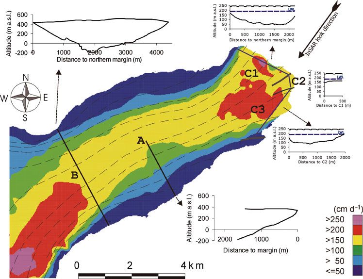
4 Stuefer and others: Climate sensitivities of Glaciar Perito Moreno
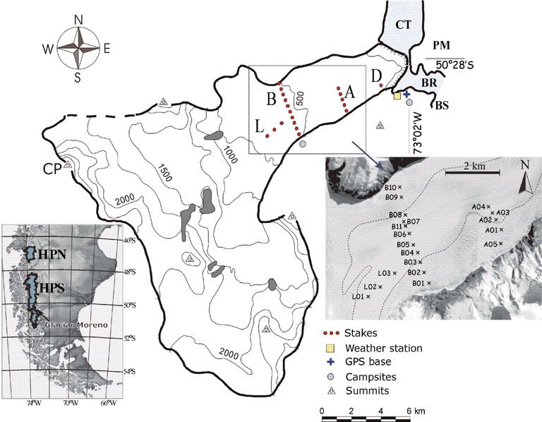
Fig. 1. Map of GPM with location of the stakes (profiles A, B, L and D), the automatic weather station, the GPS base and the campsites. The
calving front is shown as a line with dashes. CT: Canal de los Témpanos; BR: Brazo Rico; BS: Brazo Sur; PM: Penı́nsula Magallanes;
CP: Cerro Pietrobelli. The insets show an overview map with locations of the northern (HPN) and southern (HPS) Patagonian icefields, and
individual stake positions superimposed on a SPOT (Système Probatoire pour l’Observation de la Terre) image acquired on 23 August 1995;
the dashed line in the zoom inset defines the border between the smooth glacier surface of the central ablation area (zone 1) and marginal
and crevassed areas (zone 2).
This enabled us to document variations of glacier parameters Aniya, 1992). Two survey lines were set up, at a distance of
preceding the damming event. about 5 km from the glacier front. Elevation measurements
during the expeditions of 1990/91 and 1993/94 and repeat
Characteristics of Glaciar Perito Moreno and measurements in April 1996 showed no significant changes
fieldwork of ice thickness at any of the nine survey points (Skvarca and
GPM extends over a length of about 30 km from the Naruse, 1997). Later measurements showed average thick-
continental divide eastwards to Lago (lake) Argentino ening of 1.4 m a–1 at eight points in the period 1999–2002
(185 m a.s.l.) (Fig. 1). The average height of the ice divide (Skvarca and others, 2004).
is about 2200 m, with the highest point at Cerro Pietrobelli We conducted ten field campaigns between November
(2950 m a.s.l.). Based on the digital elevation data of the 1995 and October 2003, at the beginning and the end
SRTM (http://www2.jpl.nasa.gov/srtm/) and optical satellite of the three summers 1995/96, 1996/97 and 1997/98
data (Stuefer, 1999), we determined the area of GPM as (November/December and March/April), and in March/
254 km2. This is a few square kilometres less than shown in April of the years 1999–2002; the most recent campaign
previous publications, mainly due to a shift of the ice divide was in October 2003. An automatic weather station was
in the SRTM data compared to previous maps that were less installed in November 1995 on the shore of Brazo Rico,
accurate in the upper reaches of the glacier. The front 360 m from the southern front of GPM (508290 22.70800 S,
terminates with calving cliffs rising 50–80 m above the water 738020 48.00200 W; 192 m a.s.l.) (Fig. 1). The regular field-
level in Canal de los Témpanos to the north and in the work focused on the establishment and maintenance of a
southern arm (Brazo Rico) of Lago Argentino (Naruse and stake network for measurements of ice ablation and ice
others, 1992). The water of Brazo Rico discharges into the motion. In addition, we measured ice thickness using
Canal de los Témpanos through a narrow channel or below seismic reflection, and conducted echo soundings of lake
the frontal ice near Penı́nsula Magallanes. depth near the glacier fronts. Global positioning system
Previous glaciological fieldwork on GPM has been (GPS) surveys were carried out in order to map glacier
carried out, mainly near the front and on the lower part of boundaries, lake shores and peaks.
the terminus, with the first documented visit by Hauthal in
1899 (Hauthal, 1904). During the 1990s, surface motion, ice Damming of Brazo Rico
ablation, frontal position and meteorological data were GPM is noted for spectacular water outbursts after
measured during various field campaigns, usually in early damming the Brazo Rico–Brazo Sur (BR–BS) by reaching
summer, within the Japan–Argentina–Chile joint Glacio- the opposite shore at Penı́nsula Magallanes. The first known
logical Research Project in Patagonia (GRPP) (Naruse and oblique photograph of GPM showed the terminus in 1899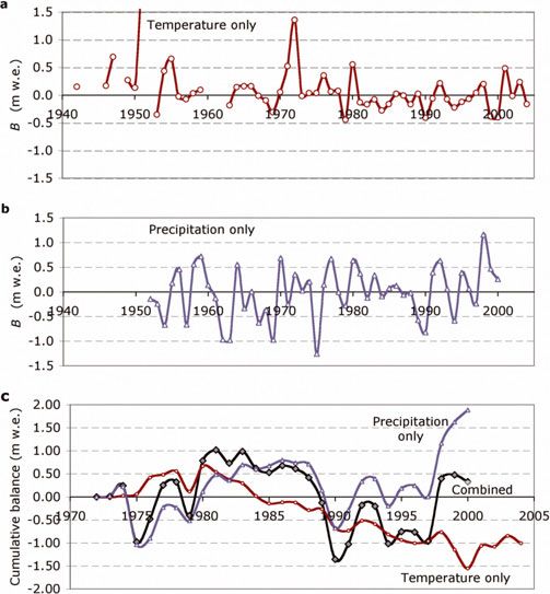
Stuefer and others: Climate sensitivities of Glaciar Perito Moreno                                                                 5

approximately 1 km above the present position (Hauthal,
1904). During the following years the glacier advanced,
inhibiting the runoff from BR–BS in 1917, the first
documented damming event (Liss, 1970). About 22 dam-
ming episodes occurred between 1917 and the present
(Heinsheimer, 1958; Aniya and Skvarca, 1992; Skvarca and
Naruse, 1997). Liss (1970) reported a maximum rise of BR–
BS water level of 28.4 m during a damming period of more
than 1.5 years from 1964 until 1965. This maximum was
not confirmed by measurements of the elevation of lower
boundaries of dense vegetation, which revealed an
estimated maximum damming height of 23.5 m above the
normal lake level (Stuefer, 1999). Water drainage over the           Fig. 2. Oblique frontal photograph of GPM, with diagram with the
low land on the northeastern side of Brazo Rico would                years of damming of BR–BS by the glacier terminus superimposed.
impede lake damming in excess of about 25 m. BR–BS was               The damming heights above a normal reference lake level are
dammed typically every 2–4 years until 1988, when                    marked for years when lake level observations are available.
damming occurred for the last time before 2003. Since
1988 the glacier front has been in an advanced position
and the glacier has repeatedly touched the opposite shore            the order of several metres at C-band if snow is dry (Rott and
at Penı́nsula Magallanes during winter, but ice tunnels              Siegel, 1997). However, in wet snow, as is the case for the
enabled runoff. Figure 2 shows the years when damming                SRTM campaign in Patagonia, the penetration depth
occurred. The maximum rise of BR–BS water level was                  amounts to only a few centimetres.
reported for a few cases, as shown in Figure 2.                         In order to obtain an independent estimate of accuracy,
   During 2003 the glacier front advanced 100–120 m in              we compared SRTM elevation data to GPS measurements at
Canal de los Témpanos and by 150 m in Brazo Rico. In                reference points in the surroundings of our meteorological
September 2003 the central part of the front of GPM blocked          station (on land) and at ablation stakes on GPM, made
the outflow from BR–BS, which consequently caused                    1 month afterwards. The mean elevation difference for
flooding of pastureland and enlarged the normal lake                 reference points on land was 0.02 m; the difference at the
surface area (150 km2) by 22 km2 (Chinni and Warren,                stakes between GPS and SRTM was, on average, 0.4 m after
2004; Rott and others, 2005). In early March 2004 the lake           correcting stake measurements by 2.1 m to account for
level of BR–BS had risen by 9.35 m (Skvarca and Naruse,             1 month’s ablation. The maximum absolute difference
2005). On 11 March 2004 the water started to drain, first            between any of the 16 GPS points and the SRTM DEM
through englacial fissures and conduits, which subsequently          amounted to 6.5 m, where these differences can be partly
evolved into an ice tunnel. Two days later a section of the ice      attributed to the different horizontal scales (point measure-
front of 60 m height collapsed.                                      ments vs 90 m grid). This comparison implies high accuracy
   Most recently, in August 2005, the ice dam has formed             of the SRTM DEM on the glacier.
again, impeding the drainage of water from BR–BS into the               The accuracy of topography from previous sources is less
main body of Lago Argentino. The rupture of the ice dam              reliable, as we found by comparing GPS measurements of
occurred almost exactly 2 years after the 2004 event. The            control points outside the glaciers (e.g. at mountain peaks)
water from BR–BS started to drain on the morning of                  with topographic maps, revealing elevation differences up to
10 March 2006, and the spectacular final collapse of the ice-        100 m (Stuefer, 1999). For comparison with SRTM, we
tunnel roof took place 3 days later, around midnight of              derived a DEM by digitizing 1 : 100 000 scale cartographic
13 March 2006.                                                       maps, based on aerial photographs taken in March 1975 and
                                                                     published by the Instituto Geográfico Militar of Argentina in
                                                                     1982. A mean vertical random error of 49 m and a mean
GLACIER GEOMETRY
                                                                     vertical bias of 9 m resulted from comparing SRTM and map
Cartography and SRTM topography                                      topography over exposed rock near GPM. GPM topography
Digital elevation data of Patagonia, including the glaciers,         derived from SRTM is consistently higher than the map
are available from the SRTM conducted in February 2000 as            topography over the glacier; taking into account the 9 m
a joint project of NASA, the US National Imagery and                 bias, the topography comparison reveals an overall thicken-
Mapping Agency (NIMA), the German Aerospace Research                 ing of 1.4 m a–1 for the period 1975–2000, with a mean
Center (DLR) and the Italian Space Agency (ASI) (http://             value of 1.9 m a–1 for the accumulation area and of 0.3 m a–1
www2.jpl.nasa.gov/srtm/). We used the SRTM standard                  for the ablation area. These data agree with the near steady
digital elevation model (DEM) at 90 m resolution, with a             state of the glacier surface in the ablation area and with the
nominal absolute vertical accuracy (90% linear error) of             observed balanced or slightly positive net mass balance over
16 m and a nominal absolute horizontal accuracy of 20 m.             recent years. However, Rignot and others (2003; online
For geocoding satellite images we interpolated the SRTM to           material at http://www.sciencemag.org/cgi/content/full/302/
a 25 m grid. This DEM is based on single-pass interferometry         5644/434/DC1, table S1) used a different 1968 map source
of the spaceborne imaging radar-C synthetic aperture radar           to derive a mean thinning of 0.42 m a–1 for 1975–2000 (total
(SIR-C SAR) system, using the C-band channel. Two per cent           of 10.5 m) for the GPM glacier area below 1650 m. The
of the GPM glacier area was not imaged by SRTM due to                different results and derived high vertical random errors
layover or radar shadow. We interpolated the elevation in            indicate that inaccuracies of available maps are too high to
these areas linearly. A possible error source for interfero-         enable a reliable quantitative comparison with SRTM for the
metric mapping over glaciers is radar penetration being of           GPM area.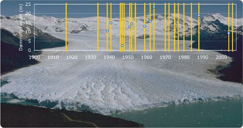
6                                                                             Stuefer and others: Climate sensitivities of Glaciar Perito Moreno

Fig. 3. Map of SIR-C/X-SAR-derived magnitude of ice velocity on the terminus of GPM. Velocity is colour-coded in steps of 50 cm d–1; the
dashed lines indicate the direction of ice flow. The insets show cross-sections along seismic/stake profiles A and B; and along C1, C2 and C3,
linear sections for calculating the calving flux; blue dashed lines show the lake water level (LWL).

Seismic measurements                                                     the northern part of the glacier bed can possibly be explained
The ice thickness of GPM was determined using the seismic                by geological differences between the opposite sides of the
reflection method along profiles A and B (Fig. 1) in Novem-              valley. The dacitic-rhyolitic volcanic rocks, which build up
ber 1996. Large parts of the profiles are crevassed and                  Cerro Cervantes in the south, probably continue below the
very rugged, and water is abundant within the ice and at                 glacier towards the centre of the profile. The mountains north
the surface. The seismic signals were recorded with a                    of the glacier are made up of black shale that is less resistant
24-channel Strataview seismograph, using two geophone                    to erosion. A second reflector shows up clearly at two-way
strings, each with 12 geophones, at a spacing of 10 m along              travel times between 0.03 and 0.15 s below the ice bottom.
lines in the direction of the profiles. The P-wave velocity was          This reflector probably represents an interface between
estimated at 3700 m s–1 by analyzing travel times of the                 subglacial sediments and bedrock.
direct P-waves between the shot points and the geophones.
                                                                         Bathymetry
This value is in agreement with measurements of wave speed
in temperate ice of other glaciers (Nolan and others, 1995;              Bathymetric measurements were carried out close to the
Nolan and Echelmeyer, 1999). The reflecting interface at the             calving fronts in Canal de los Témpanos and Brazo Rico
glacier bed was migrated using available routines from the               (Stuefer, 1999). The lake depth was measured along lines
DISCO2 software package under the assumption that the                    oriented parallel to the glacier fronts at distances 40–100 m
reflection originated in the plane of the profile.                       from the calving cliffs. The maximum depth in Brazo Rico
    The reflected seismic waves at profile A revealed a                  close to the front was 110 m, and in Canal de los Témpanos
downward slope of the glacier bed from the margin towards                the maximum depth was 164 m. The bottom depth at the
the centre line, as expected. At a distance of 1650 m from               front of section C2 in Figure 3 was estimated at 20 m below
the southern margin (almost halfway across the glacier), the             lake level by extrapolating the surface slope at Penı́nsula
farthest point reached, an ice thickness of 555 m was                    Magallanes. The height of the ice front was obtained from
measured. Subtracting this value from the surface elevation              Naruse and others (1992), who measured heights of 55–
of 360 m a.s.l. results in a depth of the glacier bed of 195 m           77 m above lake level, and from the analysis of digitized
below sea level, rising towards the calving terminus where               photographs. According to the water depth at the calving
the maximum depth of the glacier bed is 20 m a.s.l.                     fronts and the height of the ice surface above the lake level,
    Analysis of seismograms along profile B revealed a                   the glacier is grounded everywhere.
subglacial trough of approximately parabolic shape, with
the deepest part shifted to the north of the centre (inset Fig. 3).
                                                                         SURFACE VELOCITY
The average surface altitude along this transect was
495 m a.s.l. The two-way travel time of the deepest reflected            Stake measurements of velocities
signal from the interface at the glacier bottom was 0.38 s,              We used a Trimble GPS Pathfinder Pro XL in differential
corresponding to an ice thickness of 703 m (35 m) and an                mode for measuring 213 positions of ablation stakes
elevation of 208 m below sea level. The greater steepness of             between 1995 and 2003. The Trimble phase-processor
Stuefer and others: Climate sensitivities of Glaciar Perito Moreno                                                                               7

software provided horizontal point measurement accuracies
between 10 and 30 cm. For 19 stakes velocities were
measured for two summer and one winter season, and for
8 stakes at profiles A and B for six additional annual periods.
The lower transverse profile (profile A, Fig. 1) consisted of
5 stakes between the southern margin and the centre of the
glacier; the distance to the calving front was 4.5 km and the
mean elevation 360 m a.s.l. A heavily crevassed zone
prevented access to the northern part of the tongue. The
upper transverse profile (profile B, Fig. 1), consisting of
11 stakes, spanned the whole glacier width of 4.4 km at a
mean elevation of 500 m a.s.l., 7.5 km from the front. The
3 stakes of the longitudinal profile L (L01, L02, L03) were
placed along the centre line; the maximum distance to
profile B was 2.3 km (L01). The stakes were re-drilled at the
initial positions during each field campaign to obtain
comparable data for the different periods. All stakes were
found again during the following campaigns. In March 1997
the stake net was reduced to 3 stakes at profile A
(maintained until October 2003) and 5 stakes in the smooth
central zone of profile B (until March 2002).
    Figure 4 shows seasonal and mean annual deviations
from the 6 year mean velocity profiles (1996/97–2001/02)
along the transverse profiles. In the following discussion the
terms summer and winter refer to the periods defined by the
field campaigns that vary slightly from year to year (Table 1).
Annual velocities and velocities measured during winter and                  Fig. 4. Seasonal and annual deviations of surface velocities from the
summer periods are all similar. The mean annual velocity at                  6 year (1996/97–2001/02) mean profiles as derived from the stakes
                                                                             of (a) profile A and (b) profile B. The insets show mean profiles and,
A02, for example, varied between 1.05 and 1.14 m d–1
                                                                             for comparison, interferometric spaceborne imaging radar-C/X-band
during the 7 years (Fig. 4a). In the centre of profile B (B05
                                                                             SAR velocities.
and B06) the mean annual velocity varied between 1.72 and
1.84 m d–1 over the 6 year measurement period, with the
minimum in 1999/2000 (Fig. 4b). Our analysis suggests an
uncertainty of about 0.005 m d–1 in the seasonal velocities                  profile B and 8% in profile A. This ratio is contrary to the
and 0.002 m d–1 in the annual velocities.                                    longitudinal trend in magnitude of the velocity. The
    The seasonal variations were also rather small, with an                  maximum velocity, 2.39 m d–1, was measured at L01 in
average increase of velocity of only 7% during the two                       summer 1996/97.
summer periods 1995/96 and 1996/97 compared to the                              Considering the small average seasonal variability of the
winter period 1996. The summer-to-winter velocity ratio                      measured velocities and the rather stable glacier geometry,
showed a slight increase downstream, with the minimum                        no surge-type characteristics are evident. Previous measure-
difference observed in profile L (4%), followed by 7% in                     ments of ice motion on GPM were carried out at stakes in

Table 1. Mean ice ablation (cm d–1) at stakes of profiles A and B for seasonal and annual measurement periods (dd/mm/yy), separated in the
central part (zone 1) and in margin and crevasse zones (zone 2). Possible measurement errors are indicated in parentheses. From 2002 to
2003 the time lag between successive measurements was 18.5 months. Ablation values after March 1997 were measured with a reduced
stake network. The temperature is the mean value at the weather station near the glacier front over the time period

Period                                            Profile A                                        Profile B                       Temp.
                                     Zone 1                    Zone 2                 Zone 1                    Zone 2
                                                                                                                                     8C

09/11/95–18/03/96                  5.9   (1.8%)               6.5   (1.9%)          5.2   (1.7%)               6.0   (1.6%)         9.6
23/03/96–22/11/96                  1.3   (4.1%)               1.7   (3.5%)          1.2   (3.9%)               1.6   (2.8%)         5.6
22/11/96–26/03/97                  5.2   (1.9%)               6.4   (1.8%)          4.9   (1.9%)               6.0   (1.7%)         9.1
30/03/97–14/11/97                  0.9   (6.6%)               1.0   (4.5%)          0.9   (5.8%)               1.0   (4.4%)         4.2
14/11/97–22/03/98                  5.5   (2.0%)               5.6   (1.4%)          5.2   (1.7%)               6.3   (1.2%)         9.3
23/03/96–26/03/97                  2.7   (4.2%)               3.4   (3.8%)          2.4   (4.2%)               3.0   (3.7%)         6.8
30/03/97–22/03/98                  2.6   (4.9%)               2.7   (3.4%)          2.4   (4.2%)               2.9   (3.1%)         6.0
25/03/98–07/03/99                  3.2   (1.3%)               3.3   (0.9%)          2.6   (1.3%)                                    7.1
09/03/99–23/03/00                  2.8   (1.3%)               3.3   (0.8%)          2.7   (1.1%)               3.5 (0.8%)           6.9
27/03/00–15/03/01                  2.0   (1.4%)               2.5   (1.1%)          1.9   (1.7%)               2.2 (1.3%)           5.6
15/03/01–29/03/02                  2.9   (1.3%)               3.1   (0.9%)          2.4   (1.3%)               3.3 (0.8%)           6.1
05/04/02–20/10/03                  2.1   (1.1%)               2.2   (0.8%)                                                          5.5
8                                                                     Stuefer and others: Climate sensitivities of Glaciar Perito Moreno

proximity to profile A within the joint Japan–Argentina–         condition of the surface was closely fulfilled, as the 1 day
Chile project during short periods in 1990, 1993 and 1994,       ablation at the stake profile was estimated at 3–4 cm,
as well as over an annual period from November 1993 to           balancing the measured emergence velocity. In this case,
November 1994 (Naruse and others, 1992, 1995; Skvarca            surface-parallel flow can be assumed as an approximation to
and Naruse, 1997). The mean annual velocity in the centre        derive the velocity vector (Joughin and others, 1996).
of the glacier was 1.6 m d–1; velocities measured in Novem-      However, according to the shallow-ice approximation
ber/December 1993 were slightly larger than the annual           (Paterson 1994), this assumption requires surface flow to
mean 1993/94, in agreement with our observations.                be uniform over an area extending over at least ten ice
                                                                 thicknesses. Because of the complex bedrock topography,
Surface motion by means of SAR                                   this is not the case for GPM. Therefore we applied a two-step
Interferometric synthetic aperture radar (InSAR) and SAR         procedure to determine the velocity vector. The directional
amplitude cross-correlation were applied to map ice motion       flow field was derived from flowlines in SAR images,
in the ablation area. These data contributed to retrieving       Landsat images and aerial photography. The local verifica-
mass fluxes and to studying the flow behaviour of the            tion with stake measurements showed good agreement.
terminus. The multi-year field measurements at the stakes        Using the LOS velocity field, the directional flow field and
provide a baseline to determine the representativeness of        the surface slopes along the flowlines, the velocity vector
the short-term velocities from satellite data. Because of the    was derived. Because of the small surface slope in the
fast flow of GPM, SAR images of short time-spans (a few          ablation area, the magnitude of the vertical velocity is
days maximum) are required for InSAR motion analysis to          typically of the order of 3–5% of the horizontal velocity. For
avoid phase decorrelation in shear zones (Zebker and             the image section near the heavily crevassed calving front,
Villasenor, 1992).                                               we calculated displacement in azimuth and range by
   The best interferometric dataset of GPM so far available      correlating L-band amplitude data from the 3 day repeat
was acquired on 7, 9 and 10 October 1994 by the space-           image pair of 7 and 10 October 1994.
borne imaging radar-C/X-band SAR (SIR-C/X-SAR) that                  Figure 3 shows a map of the SAR-derived motion field of
operated on board the space shuttle Endeavour (Stofan and        the terminal 12 km of GPM. This map reveals some
others, 1995). We used L-band ( ¼ 24.23 cm) repeat-pass         differences to the previously published velocity map (Rott
images, with a resolution of 8.2 m in azimuth (along-track)      and others, 1998) because more precise orbit data and a
and of 3.8 m in slant range (direction of the radar beam), and   larger set of geodetic field data are now available, enabling
radar look angle from the vertical of 34.48 at the image         more accurate geocoding. The main mass input to the
centre. C- and X-band repeat-pass images decorrelated over       ablation area is supplied through the southern ice stream,
the glacier due to surface melt. Close to the calving front,     which drains an area 100 km2 and is only 1.4 km wide
L-band images also decorrelated, even over the 1 day time-       near the equilibrium line. In this area, 5 km southwest of
span because of chaotic displacement of seracs. In this          stake L1 (Fig. 1), a velocity maximum of 3.5 m d–1 was
section of the terminus, we applied amplitude correlation in     derived by means of cross-correlation. In this area the
the across-track and along-track directions to map the           fractured surface is reminiscent of a surging glacier, though
motion. This method is less accurate than InSAR, in              this is probably not the case. In the lower part of the
particular if the repeat-pass time-span is short (Gray and       terminus the velocity shows a minimum near profile A, and
others, 1998; Pattyn and Derauw, 2002). Michel and Rignot        increases towards the front due to converging flow and a
(1999) calculated the motion field of the lowermost 4 km of      rising glacier bed.
the Moreno terminus in radar geometry, applying a combin-
ation of coherent and non-coherent image correlation using       Comparison of motion from InSAR, amplitude
the L-band image pair from 9 and 10 October 1994.                correlation and field data
   An important step for interferometric retrieval of surface    The velocities from the two different SAR analysis tech-
displacement is the separation of the topographic phase and      niques and from the geodetic field measurements show
the motion-related phase (Mohr and others, 2003). Because        good agreement. Over the central part of the terminus a
only one InSAR pair of good coherence (9/10 October 2004)        standard error estimate est ¼ 9 cm d–1 in ground range was
was available, it was necessary to generate a synthetic          derived between motion from interferometry and from
topographic interferogram using a DEM and orbit par-             cross-correlation, based on linear regression of more than
ameters. At the given incidence angle and interferometric        3000 samples with a degree of coherence above 0.4 for the
baseline of 29 m, one interferometric fringe ( ¼ 2)           1 day image pair. The main part of this error can be
corresponds to an altitude difference of 620 m (the altitude     attributed to the cross-correlation analysis because the
of ambiguity, Ha) or to a displacement of 12.1 cm in line of     sensitivity of this method is related to range and azimuth
sight (LOS) of the radar beam. Because of the high value of      resolution and is therefore lower than for InSAR.
Ha and the gentle topography of the Moreno terminus,                For comparison of SAR-derived velocities with field data,
possible errors in the DEM have little impact on the retrieved   the different observation periods have to be considered. SAR
interferometric velocity.                                        provides the motion for a 1 day or 3 day time interval in early
   As InSAR provides only the LOS component of the               summer 1994, whereas the field measurements were made
velocity vector, assumptions about the flow direction are        over seasonal or annual periods, starting in summer 1995.
necessary in order to use the data for ice dynamic studies       The interannual velocity variations during the period 1995–
(Joughin and others, 1996; Reeh and others, 1999; Mohr and       2003 and the seasonal variations amount to a few per cent
others, 2003). On the GPM terminus, surface topography           variation. Because we use the SAR data for estimating
was very close to steady state over annual intervals, as known   annual mass fluxes, we compared the SAR motion fields
from geodetic field measurements (Stuefer, 1999). Also for       with the mean annual velocities derived from the stake
the 1 day interval of 9–10 October 1995 a steady-state           network (compare insets of Fig. 4). Excluding stakes at the
Stuefer and others: Climate sensitivities of Glaciar Perito Moreno 9
Fig. 5. Winter, summer and annual ice ablation for four stakes of the central profile B from 1995 to 2002. Inset: Annual ablation values from
April to March for zone 1 (profiles A and B) and zone 2 (profile A). The red line indicates mean temperatures for corresponding time periods.
glacier margins where the flow direction deviated more than The year 2000/01 had the lowest ablation, deviating by
608 from ground range, a standard error est ¼ 5 cm d–1 was –21% from the 7 year average and coinciding with the
derived between the short-term interferometric and the comparatively low mean annual temperature of 5.68C
annual velocities measured by differential GPS at the recorded at Moreno weather station. The variability between
individual stakes after subtracting the mean bias of 3.6% the three observed summer periods was rather small. This is
between the SAR and GPS measurements. This bias, where in agreement with the small differences of mean summer
the higher values correspond to SAR velocities, can be temperatures and the slightly higher variability of mean
explained by slightly increased velocity in summer. annual temperatures (Table 1). Previous ablation measure-
ments, carried out at four positions close to profile A in
summer 1993/94 within the GRPP (Naruse and others,
ABLATION MEASUREMENTS 1995), show values similar to our 7 year measurements in
Between November 1995 and October 2003, ice ablation that area.
was measured at the wooden stakes of profiles A–C. One Air-temperature data, shown in Table 1 and Figure 5,
additional stake (stake D) was drilled 500 m from the ice were measured at the weather station near the glacier
front at Brazo Rico, 70 m from the southern glacier margin. terminus and used for modelling of ablation. A second
Ice may melt in any season because, even in winter, the temperature probe was installed in April 2002 close to the
lower terminus is often free of snow and the air temperature glacier margin, 400 m above the main station, which
may stay above 08C over extended periods. The ablation recorded over a period of 18 months. A mean vertical lapse
measurements revealed obvious differences between stakes rate of temperature of 88C km–1 was derived (comparable to
located in marginal and crevassed zones (zone 2, containing Takeuchi and others, 1996) for the calculation of positive
the stakes A05, A01; B01, B02, B03, B09, B10) and stakes in degree-days for each stake elevation and measurement
the central part of the glacier (zone 1) that is rather smooth period. Figure 6 shows all seasonal and annual ablation
(Fig. 1). Zone 2, showing higher ablation, is characterized by measurements in relation to the corresponding positive
slightly lower surface albedo and/or rather high crevasse degree-day sums; the lines illustrate the best linear fit for
density. Ablation measurements and their relative errors for different seasons and surface zones. Mean degree-day
the observation periods and ablation zones are summarized factors during summer periods amount to 0.61 cm water
in Table 1. The relative errors for seasonal or annual periods equivalent per positive degree-day (cm w.e. 8C–1 d–1) in
are small due to high ablation sums. The mean ice ablation zone 1 of profile A and to 0.64 cm w.e. 8C–1 d–1 in zone 1
of the three summers in zone 1 amounted to 5.5 cm d–1 at of profile B. The values for zone 2 are 0.68 cm w.e. 8C–1 d–1
profile A, and 5.1 cm d–1 at profile B. The corresponding (profile A) and 0.76 cm w.e. 8C–1 d–1 (profile B). These values
mean values of the two winter periods were 1.1 and are comparable to those of other glaciers in maritime
1.0 cm d–1, and the mean values over the 6 year period regions (Braithwaite and Zhang, 2000). For winter periods
March 1996–March 2002 were 2.7 and 2.4 cm d–1. On the degree-day factors shown in Figure 6 consider exclu-
average, in profile A the ablation in zone 2 was 11% higher sively ice ablation and do not account for snow fallen and
than in zone 1, and in profile B it was 18% higher. The larger melted; the derived values vary between 0.27 and
difference at profile B is probably an effect of the very rough 0.43 cm w.e. 8C–1 d–1. Annual values (Fig. 6a) result from
glacier surface of zone 2, characterized by a maze of ice field measurements in the years 1998/99 to 2001/02, when
ridges and troughs with a typical vertical scale of 10 m. seasonal data were not available for this study. Ablation was
The mean ablation of the five central stakes at profile B for measured at stake D at short intervals during summer 1995/
the different observation periods is illustrated in Figure 5. In 96; the ablation data show a clear linear relation to
summer, the variability between the individual stakes, temperature (Fig. 6b). The degree-day factor at stake D of
mainly caused by local variations of surface roughness, 0.79 cm w.e. 8C–1 d–1 is slightly higher than the long-term
was slightly higher than the interannual variability. The inset summer factors at zone 2, probably due to the closeness to
of Figure 5 shows annual ice ablation for the different zones. the glacier margin (Stuefer, 1999).10 Stuefer and others: Climate sensitivities of Glaciar Perito Moreno
To retrieve Bac the total glacier area, S, was separated into
the accumulation area, Sac, and the ablation area, Sab, using
the average position of the equilibrium line inferred from
positions of the snowline in late summer of the years 1986
and 1993–2005. The database includes one Landsat The-
matic Mapper (TM) image of 1986, several ERS (European
Remote-sensing Satellite) SAR images of 1993, 1995, 1996
and 1998, Envisat Advanced SAR (ASAR) images of 2003,
2004 and 2005, a RADARSAT image of 1997 and oblique
photography from March 1994, 1999 and 2000. During the
various field campaigns in late summer, which lasted up to
3 weeks, we observed little variability of snowline position.
Reasons for this are probably the steepness of the glacier
surface at the equilibrium line and frequent snowfalls,
resulting in small interannual variability of the accumu-
lation-area ratio (AAR). This suggests that the equilibrium line
can be inferred with good accuracy from mean snowline
positions at the end of several summers. We estimate the
mean equilibrium-line altitude (ELA) as 1170 m a.s.l., in
close agreement with the ELA of 1150 m a.s.l. derived by
Aniya and others (1996). This results in an accumulation area
of 177.5 km2, corresponding to an accumulation-area ratio
(AAR ¼ Sac/S) of 70.0%. The mean snowline altitude at the
end of the 12 summers varied by 70 m at maximum, which
corresponds to a variation of the AAR between +2% and
–2.5% of the mean value.
The surface ablation, Bab, was calculated by means of
linear altitude gradients of net balance, separating the
ablation area into a central region (zone 1) with an area
Sab,1 ¼ 35.6 km2 and the marginal and crevasse zones
(zone 2) with Sab,2 ¼ 40.9 km2. The zone extent was
mapped from Landsat images, air photos and GPS measure-
ments. The balance gradients, 1 ¼ 11.47 kg m–2 a–1 m–1
and 2 ¼ 14.39 kg m–2 a–1 m–1, derived from the measured
Fig. 6. (a) Seasonal and annual positive degree-days vs measured mean annual ablation (Table 1), are characteristic for
ablation. Note: The ablation data and degree-day factors (ddf) maritime glaciers and indicate high mass turnover (Oerle-
indicating the slope of the individual trend lines refer to ice mans and Fortuin, 1992). A mean surface balance bB,1 ¼
ablation. Values have been converted to centimetres water equiva- –7688 kg m–2 a–1 was calculated for zone 1 and bB,2 ¼
lent (cm w.e.) in the text. (b) Ice ablation and corresponding degree-
–9640 kg m–2 a–1 for zone 2, assuming ¼ 900 kg m–3. For
days at stake D measured for daily and short-term periods during
151 days in austral summer 1995/96.
the crevassed area near the front we calculated a maximum
ablation (bmax,2) of –14 245 kg m–2 a–1, corresponding to an
ice ablation of 15.8 m a–1. A net balance Bab ¼ –0.544 Gt a–1
resulted for the total ablation area, and Bab1 ¼ –0.243 Gt a–1
GLACIER MASS FLUXES for the area between profile B and the equilibrium line.
Field measurements and satellite data analysis were the basis The seismically derived cross-section and surface velocity
for retrieving total net ablation and mass fluxes. Rott and measurements were the basis for calculating the ice
others (1998) presented first estimates of mass-balance discharge, Mt, through profile B:
components under the assumption that GPM is close to Z WB
equilibrium state, based on 2 years of field measurements. Mt ¼ um ðy Þhðy Þ dy: ð2Þ
0
However, because of the longer response time of a glacier,
the quasi-steady-state assumption should be applied over a The y coordinate is aligned along the transverse profile, and
multi-year period, so that interannual variations are filtered um(y) is the mean horizontal velocity normal to the profile
out. This was enabled by extension of the observation period. in a vertical column of ice; h(y) is the depth and WB the
Because of the size of the accumulation area, the difficult profile width. Simple shear flow with the shear stress xz
access, the high accumulation rate and the high spatial (xz ¼ fgðh zÞ sin ) depending on the surface slope, ,
variability due to strong winds, it was not feasible to and the weight of ice above (gðh zÞ) is assumed,
measure the total net accumulation, Bac, in the field. We following Paterson (1994), for estimating the dependence
therefore estimated Bac by the following relation, assuming of velocity on depth. We used ¼ 2.58, the average slope
conservation of mass, over a distance of 5 km normal to the profile, and shape
factor f ¼ 0.75, valid for a parabolic channel and the
Bac ¼ Bab1 M t : ð1Þ
measured ratio of ice depth to glacier width. For describing
Bab1 is the net ablation in the area between the equilibrium the ice flow, Glen’s flow law (du=dz ¼ 2Axz n
) with par-
line and profile B, and M t is the mass flux through the glacier ameters n ¼ 3 and A ¼ 3.8 10 Pa s was used, where
–24 –3 –1
cross-section at profile B. A represents a mean of values reported for temperateStuefer and others: Climate sensitivities of Glaciar Perito Moreno 11
glaciers by Gudmundsson (1994) and Paterson (1994). Table 2. Characteristics of the three sections of the calving front of
Integration of the flow law from the surface (z ¼ hc) to the GPM; h is the mean ice thickness, ucentre the magnitude of the mean
bed (z ¼ 0) yields (Paterson, 1994) annual calving velocity in the centre of the profile, ucv the width-
Z averaged calving rate and Bcv the calving flux
1 hc
umc ¼ usc n
2Axz dz: ð3Þ
hc 0 Section Width h ucentre ucv Bcv
For ¼ 900 kg m and the measured depth in the centre,
–3
m m ma –1
ma –1
10 kg a–1
9
hc ¼ 703 m, a mean velocity, umc, amounting to 0.9 times
the surface velocity, usc, was derived. We used the same C1 2300 165 795 715 –244
factor of 0.90 for the total cross-section, representing the C2 500 96 662 509 –22
mean between zero and full sliding. The resulting mass flow C3 2100 119 606 420 –95
through the profile is M t ¼ –0.727 Gt a–1. With the values
for Bab1 and M t we estimate the net accumulation accord-
ing to Equation (1) as Bac ¼ 0.970 Gt a–1. This corresponds
to a specific annual net accumulation bac ¼ 5465 mm
w.e. a–1. With a conservatively estimated accuracy for Bab1 significantly higher than the derived net accumulation of
of 20% and for M t of 10%, the uncertainty of bac is 5465 mm w.e. a–1. This conclusion is in agreement with the
480 mm w.e. a–1. estimates of Schwerdtfeger (1958) and Escobar and others
An estimate of the calving flux, Bcv, provided an (1992). Schwerdtfeger estimated the annual precipitation
additional control for the assumption of a quasi-steady state above 1500 m a.s.l. to be at least 1.5–2 times the precipi-
of the glacier and for estimating errors of the various fluxes: tation measured at the coastal weather stations, which
would correspond to an annual precipitation sum of at least
M t ¼ Bab2 þ Bcv þ Br : ð4Þ
7000 mm on the western side of HPS. Escobar and others
Bab2 is the surface melt loss in the area below profile B, and (1992) estimated the mean annual precipitation for the
the residual, Br, accounts for errors of Bab2, Bcv and M t, whole HPS at 7000 mm and for the central plateau of the
and/or deviations from the state of equilibrium. icefield at more than 8000 mm. These values were inferred
For calculating the ice export due to calving, the front was from an estimation of the water balance. Aristarain and
separated into three linear sections, the section in Canal de Delmas (1993), however, derived a mean annual water
los Témpanos (C1), the section in front of Penı́nsula equivalent of 1200 mm from deuterium analysis and stratig-
Magallanes (C2) and the section in Brazo Rico (C3) raphy of a 13 m firn core that was drilled at 2680 m a.s.l.
(Fig. 3). For each section we estimated Bcv according to: near the ice divide of GPM. A possible explanation for this
Z low value may be reduced accumulation due to wind drift
Bcv ¼ ½ucv ðy Þhðy Þ dy, ð5Þ near the continental divide.
y
where ucv is the velocity normal to the calving front, h is the
ice thickness at the front, and the y coordinate is aligned GLACIER SENSITIVITY TO CLIMATE
parallel to the front. The calving speed, ucv, was taken from Seasonal sensitivity characteristics and monthly parameters
the velocity map (Fig. 3), reducing the SAR velocities by 4% for temperature sensitivity are estimated using a simple
to represent the annual mean. The calving fluxes, Bcv, the degree-day model (Oerlemans and Reichert, 2000). Daily
velocity magnitudes at the centre, ucentre, and the mean mean temperatures from Moreno base station serve as model
calving velocities, ucv (Bcv divided by the profile cross- input to reconstruct GPM mass balance. A linear relation of
section) are specified in Table 2. The lowest calving speed perturbations in precipitation and temperature to glacier
is observed at profile C3, because this front is aligned mass balance is assumed and mutual interference of
oblique to the main ice flow upstream. For the profiles C1 monthly perturbations is ignored. The main inaccuracies in
(ucv/d ¼ 6.4) and C3 (ucv/d ¼ 6.5) the ratio of calving modelling mass balance of Patagonian glaciers arise from
velocity to lake depth, d, is significantly higher than the the lack of knowledge of precipitation distribution. Precipi-
average ratio of 2.5 reported for freshwater calving by Funk tation measurements at two adjacent sites within 5 km of the
and Röthlisberger (1989). Much higher ratios were also Moreno terminus during summer 1996/97 showed signifi-
reported for the nearby Glaciar Upsala (Skvarca and others, cant differences, reflecting the influence of the strong winds
2002). A total calving flux of –0.361 Gt a–1 was calculated on precipitation measurements with conventional methods
assuming perfect sliding. This number includes the ice (Stuefer, 1999). Carrasco and others (2002) pointed out a
export and frontal melting. The main part (68%) of the homogeneous distribution of precipitation throughout the
calving flux is discharged through the frontal section, C1. year at several weather stations on the west and east sides of
These numbers differ slightly from Rott and others (1998) HPS; precipitation occurs at some stations on the wind-
due to re-analysis of the velocity field and the slight shift of exposed west side of HPS on 90% of all days. For our
the calving profiles. model we assume precipitation to occur on every day of the
If we compare M t with the independently calculated year. Lacking other more accurate precipitation measure-
numbers for surface ablation below profile B (Bab2 ¼ Bab – ments in the glacier vicinity, we used a precipitation
Bab1 ¼ –0.301 Gt a–1) and the calving flux Bcv (Equation (4)), climatology (VASClimO) compiled by an initiative of the
a residual term, B r, of –0.065 Gt a–1 results, that is within the German Weather Service and the Johann Wolfgang Goethe
estimated error bounds. Taking into account that some of the University Frankfurt (Beck and others, 2005). The monthly
snow and rain deposited in the accumulation area is lost as precipitation dataset from 1951 to 2000 is based on quality-
runoff, in particular in the area close to the equilibrium line, controlled station data. The grid data derived from the few
it can be assumed that the average annual precipitation is precipitation records that are available in the vicinity of HPS12 Stuefer and others: Climate sensitivities of Glaciar Perito Moreno
0.970 Gt a–1, which was derived from mass flux considera-
tions assuming a quasi-steady state of the glacier. The
parabolic distribution of precipitation accounts for assumed
large amounts of drifting snow, especially in the region
below the main divide due to the prevailing strong westerly
winds (Woo and Fitzharris, 1992).
Figure 7 illustrates the annual specific balance for GPM
for the example balance year 1999/2000. The maritime-
like setting of GPM with high mass turnovers is expressed
by the magnitude of balance ranging from about –18 to
+7.6 m w.e. a–1. The almost linear balance gradients derived
for the lower ablation area of GPM (below 1000 m a.s.l.)
amount to 1.65 m w.e. (a 100 m)–1 for zone 1 and 1.88 m w.e.
(a 100 m)–1 for zone 2. It is evident from the temperature
record that at higher regions ablation plays a minor role, and
that precipitation above the ELA falls predominantly as
snow; the model shows almost no ablation above 2000 m.
Fig. 7. Calculated mass-balance profile for the balance year 1999/ The strong increase of accumulation above the ELA reflects
2000 (black line). The dashed lines indicate profiles of temperature
the precipitation pattern. A high sensitivity of changes in
ablation and accumulation due to precipitation. The effects of
total mass balance to temperature and precipitation
uniform increases in temperature (+18C) and precipitation (+10%)
on the mass-balance profile are shown by the grey lines. perturbations is derived using Oerlemans’ concept of
seasonal sensitivity characteristic (SSC) parameters CT,k and
CP,k (Oerlemans and Reichert, 2000). With the index k
denoting a specific month, the balance, B, sensitivities for
do not resolve the detail of the strong precipitation gradients temperature, T, and precipitation, P, perturbations were
due to topographic effects of the Andes. In the absence of defined as
other long-term sources, we used monthly data from the @B
closest gridpoint (50.58 S, 73.58 W) as proxy for the precipi- CT, k ¼
@Tk
tation at Moreno base. The gridpoint data show maximum
and
precipitation from May to July (between 104 and 98 mm
@B P
monthly precipitation for the months May, June and July) CP, k ¼ k : ð6Þ
and minimum precipitation (46 mm) in February; the annual @ Pref, k
mean precipitation sum from 1951 to 2000 was 838 mm For the monthly sums of precipitation in the reference case
(with a standard deviation, , of 102 mm). (Pref,k) we used the 1951–2000 average of the closest
In our model, snowfall is accumulated, while rain or water gridpoint of VASClimO data (Beck and others, 2005). The
formed from melting is assumed to drain without balance effects of 18C temperature and 10% precipitation perturba-
effects. Melting of snow or ice is calculated with the positive- tions on the specific mass balance of GPM are shown in
degree-day concept. As daily mean temperatures and daily Figure 7. For the period 1996–2003 we observed differences
sums of precipitation serve as source data, the model does in mean annual temperatures of 18C at Moreno base. High
not consider changes of state in the course of a day. We sensitivity to temperature persists throughout the ablation
inversely derived a threshold of 28C daily mean temperature area. Temperature perturbations of 18C result in total
to decide whether precipitation falls as snow or rain. Further mean mass-balance changes of 0.8 m w.e. a–1, and at
model parameters are degree-day coefficients, for which we altitudes below 700 m in changes of balance of more than
take into account the two roughness zones described 3 m w.e. a–1. The hypsometry of GPM accounts for a small
previously and whether the surface is ice- or snow-covered. temperature influence on mass balance above the ELA. A
Degree-day factors over ice amount to 0.65 cm w.e. 8C–1 d–1 reversed effect is derived for precipitation perturbations,
for zone 1 and to 0.74 cm w.e. 8C–1 d–1 for zone 2 directly with gradually increasing precipitation sensitivities from the
from the average of ablation stake measurements during ELA up to altitudes of 2000 m. The higher glacier regions
summer periods. Degree-day coefficients over snow have experience balance changes almost directly proportional to
been adjusted to get the best fit of observed to modelled changes in precipitation. Monthly perturbation sensitivities
data. In addition, parameters are adjusted to account for an are illustrated in analogy with Oerlemans and Reichert’s
approximate ELA of 1170 m. Using winter degree-day figure 1 (2000) in Figure 8. Though the temperature
factors of 0.3 cm w.e. 8C–1 d–1 for both surface zones and a sensitivity is slightly less pronounced, we found SSC for
linear precipitation increase with altitude of 15% per 100 m GPM similar to Franz Josef Glacier, New Zealand. Franz
up to the ELA, a regression coefficient of R2 ¼ 0.86 is Josef Glacier is located in a maritime climate comparable to
derived between modelled balance and all 103 observed GPM, with annual precipitation values amounting to about
stake measurements; the standard error of modelled ablation 6 m (Oerlemans, 1997). Temperature effects dominate from
is 17%. As a first estimate the altitude increase of precipi- September to April, with SSC values up to 0.12 m (month)–1
tation above the ELA was approximated as a parabola for temperature perturbations of 18C. There is still a
defined by the precipitation at the ELA and an assumed significant temperature SSC in winter as melting and rain
precipitation of 7600 mm w.e. at 2500 m with the same may occur throughout the year at the glacier terminus. GPM
value up to the top of the Moreno catchment area (2950 m). SSC values for precipitation increase towards winter, with
This maximum precipitation was inversely determined to maximum values of 0.045 m (month)–1 for 10% precipi-
obtain a total net accumulation on GPM of about tation perturbation.Stuefer and others: Climate sensitivities of Glaciar Perito Moreno 13
Fig. 8. SSCs for GPM for 18C temperature and 10% precipitation
perturbations as derived from degree-day model calculations.
DISCUSSION OF MASS-BALANCE TRENDS
Monthly balance sensitivities of GPM are used to estimate
long-term trends of mass balance. A constant value for the
calving flux is assumed, which can be justified by the
Fig. 9. (a, b) Long-term specific balance derived from a degree-day
observed long-term stability of the glacier front and the small
model using the SSC and monthly temperature (a) and
annual variations of surface velocities. Various sources of precipitation (b) perturbations. (c) Cumulative mass balance from
meteorological data serve as input for the balance estimates. 1973 to 2004 as calculated from monthly temperature and
Homogeneous long-term climate observations are sparse in precipitation data separately, and the resulting combined cumu-
Patagonia, resulting in uncertainties for establishing relations lative mass balance.
between HPS glacier changes and possible climate trends.
For GPM the closest weather station is Lago Argentino station
located 60 km to the east of the glacier, operated by the
Argentine Meteorological Service. Climatic records are avail- years after 1973 the cumulative balance is shown for the two
able from 1937, although there are several gaps in the series. separate terms, as well as for their combined effect. Except
In 2001 the station was moved from El Calafate town to the for two extremely cold years (1951 and 1972), perturbations
newly built airport about 30 km to the east. The warming in temperature modulate the mass balance typically within a
trend south of 468 S during the 20th century, reported by range 0.5 m w.e. a–1. For the precipitation effect, higher
Hoffmann and others (1997), is not evident in the tempera- annual mass-balance variability is evident (Fig. 9b). The
ture data of Lago Argentino station. Carrasco and others cumulative mass balance derived from temperature pertur-
(2002) also describe a general warming trend in the vicinity bations shows balanced or positive annual mass balance up
of HPS during the last 100 years, but point out considerable to 1980. A slight but fairly consistent negative trend
variability from station to station. They present examples of amounting to a total of about 2 m w.e. follows until the year
stations where the trend reversed in the 1980s with slightly 2000. From 2000 to 2004 the temperature effect triggers a
decreasing air temperature and increasing precipitation. positive or approximately balanced state of the glacier. The
For reconstruction of mass balance we used the SSC for combined effects for the last 30 years result in negative
GPM and monthly mean temperatures measured at Moreno balance from 1989 to 1998 (Fig. 9c). Later increased
base and Lago Argentino. Moreno base monthly tempera- precipitation compensated for the partly negative balance
tures were derived by linear regression from the Lago trend from temperatures. Though precipitation estimates are
Argentino temperature series from 1941 with few gaps. The less accurate than temperature measurements, and the
comparison of the mean temperatures for 60 months absolute numbers of mass-balance variations should be
between January 1996 and December 2000 resulted in high considered with reservations, the SSC estimates clearly show
linear regression (R2 ¼ 0.97) between the two stations. For that the mass-balance behaviour of GPM was determined
the mass-balance dependence on precipitation we used the similarly by temperature and precipitation. The simulations
monthly data from the closest gridpoint of the 1951–2000 suggest that the repeated damming of BR–BS in 2003/04 and
VASClimO precipitation climatology (Beck and others, 2005/06 is the response to a few years of positive mass
2005). The SSC method applies relative changes of precipi- balance due to a combined effect of mass excess resulting
tation (Pk/Pref,k) to derive monthly changes in glacier mass from slightly colder temperatures and higher precipitation.
balance (B). Therefore VASClimO precipitation data were No damming was observed during the 1990s (Fig. 2), as the
used directly as an estimate for reconstructing the precipi- minor precipitation excess could not compensate for the
tation contribution to GPM balance changes. negative mass balance triggered by slightly increased
Resulting specific annual balance (with the balance year temperatures. In general, the derived amplitudes of cumu-
from 1 April to 31 March of the following year) is plotted in lative mass balance of GPM varied within a small range of
Figure 9 for all available years of climate data, separately for 2 m w.e. during the last 30 years, which agrees with the
temperature- and precipitation-controlled effects. For the observed balanced state of the glacier.You can also read