Periodicity in Extreme Weather in the 'Maritime Region' of Eastern North America - Research Square
←
→
Page content transcription
If your browser does not render page correctly, please read the page content below
Periodicity in Extreme Weather in the ‘Maritime
Region’ of Eastern North America
Carling Ruth Walsh ( carling.walsh@carleton.ca )
Carleton University
R. Timothy Patterson
Carleton University
Research Article
Keywords: extreme weather, solar AMO NAO AO ENSO QBO teleconnections, climate change, eastern
North America, Maritimes, time series analysis
DOI: https://doi.org/10.21203/rs.3.rs-280154/v1
License: This work is licensed under a Creative Commons Attribution 4.0 International License.
Read Full License
Page 1/36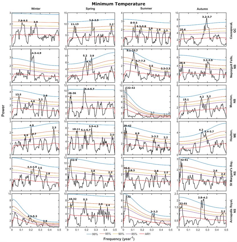
Abstract
Spectral and wavelet analysis were used to identify trends and cycles in extreme temperature and
precipitation events based on historical data (~100-150 years) from six climate stations within the
“Maritime Region” of eastern North America. Many statistically signi cant climate cycles were identi ed
using both spectral and Morlet wavelet analyses at each of these locations for both extreme high and low
temperature and precipitation (rain, snow) data, with periodicities typically ranging from ~ 2–30 years. To
assess potential drivers of these cyclical extreme weather events, the records of these events were
compared, using cross wavelet analysis, to the climate indices of several teleconnections, including the
11-year Schwabe solar cycle, Atlantic Multidecadal Oscillation, North Atlantic Oscillation, Arctic
Oscillation, El Niño Southern Oscillation and the Quasi–Biennial Oscillation. It was found that the 11-year
solar cycle had the strongest in uence over extreme temperature and precipitation in this region, whereas
the remaining oscillations, with the exception the Quasi–Biennial Oscillation, exhibited complex
interactions with one another, characterized a variety of both positive and negative modulating effects.
The Quasi–Biennial Oscillation was found to drive high–frequency oscillations in extreme weather,
particularly extreme precipitation. Overall, the ndings of this study indicate that extreme weather events
in this region have not substantially increased or decreased in number over time, but have been
predominantly in uenced by several cyclic climate phenomena.

Introduction
Historically, extreme weather events have posed undeniable risk and consequence to both humans and
the environment (Parmesan et al. 2000; Greenough et al. 2001; Znachor et al. 2008; Ummenhofer and
Meehl 2017; van de Pol et al. 2017; Campbell et al. 2018; Smith and Sheridan 2019) and have been
considered among the highest global risk factors in terms of both likelihood and impact (World Economic
Forum 2019). Unlike seasonal weather changes, extreme weather events occur within considerably
shorter time frames, rendering them nearly impossible to adapt to which, in turn, can be detrimental to
human and ecological health (e.g. heat waves associated with increased emergency medical needs
(Dolney and Sheridan 2006); storm-induced disturbances distressing phytoplankton communities
(Stockwell et al. 2020)).

Changing patterns in the frequency and intensity of extreme weather events driven by anthropogenically
driven climate change potentially represents yet another factor to be considered when developing future
risk assessment scenarios. Indeed many studies have already reported evidence of increased frequency
and intensity in extreme events (e.g. Rahmstorf and Coumou 2011; Gao et al. 2012; Wang et al. 2015),
and based on these results computer modeling predicts a concomitant increase in medical and
environmental impacts (Wu et al. 2014; Oliver et al. 2019). In contrast, other researchers suggest that
natural cyclic climate oscillations within the relatively short historical climate record dataset is a primary
in uence on the frequency of extreme events (e.g. Knight et al. 2006; En eld and Cid-Serrano 2010).

                                                   Page 2/36
With models forecasting an increase in the frequency of extreme weather throughout North America and
other mid–latitude regions, (Cai et al. 2014; Cohen et al. 2014; Wang et al. 2015) analysis of regional data
subsets of extreme weather events provide an opportunity to speci cally assess more localized trends
and cycles, and to ascertain whether they are widespread throughout a given region. Furthermore, such
analyses provide an opportunity to directly compare instances of extreme weather to various documented
cyclic climate phenomena to determine whether cyclical phenomena constitute localized or regional
drivers of extreme weather events. Developing such a regional-scale understanding of the contributors to
extreme weather is important to society as localized instances of extreme weather can result in ood
damage, dangerous road conditions, increased risk of temperature–related health concerns (e.g. heat
stroke, frost bite), and may ultimately be related to a myriad of health and safety hazards, as well as a
broader ecological impact (Bouwer 2019).

Understanding whether there are trends and cycles in the occurrence of extreme weather events can also
provide important information on changes in climate dynamics, an important metric when measuring
overall climate change (Linnenluecke et al. 2012; Moazami et al. 2019). Analysis of extreme weather
phenomena has also received increased scrutiny within the climate change research community in recent
years as new information on the broad impacts of extreme weather has emerged (Ummenhofer and
Meehl 2017; Bouwer 2019)

This study examined trends and patterns in daily extreme high and low temperature and precipitation
(rain, snow) in eastern North America, speci cally a regional subset informally dubbed here as the
Maritime Region (MR; see section 4.3 below) and comprising historical weather records from 24 stations
in New Brunswick, Nova Scotia, Prince Edward Island, eastern Maine and the Gaspé region of Quebec.
Historical records selected for detailed analysis in the MR comprised stations with near-continuous
instrumental data records spanning the past 100–150 years. Spectral, Morlet wavelet and cross wavelet
time series analysis techniques were then employed to detect trends and patterns within individual
records, and to determine whether they correlate with trends and cycles in the records of known drivers of
climate in the region (Bonsal and Shabbar 2011; Patterson and Swindles 2015).

Previous Work
Most previous studies that have examined extreme weather phenomena within or near the MR study area
have not been carried out to understand the nature of extreme weather itself, but instead have principally
either assessed the impact of these events on the environment factors (Payette et al. 1985; Scott et al.
2003; Boland et al. 2004; Andalo et al. 2005; Nye et al. 2009; Ugarte et al. 2010; Lemieux and Scott 2011),
or have focused on the in uence of extreme weather on human health and safety (Andrey et al. 2003;
Dolney and Sheridan 2006; Ziska et al. 2008; Balbus and Malina 2009; Cheng et al. 2012; Wu et al. 2014).

Amongst the few studies that have focused on the incidence of extreme weather phenomena Douglas
and Fairbank (2010) for example, examined trends in extreme precipitation in New England, nding that

                                                  Page 3/36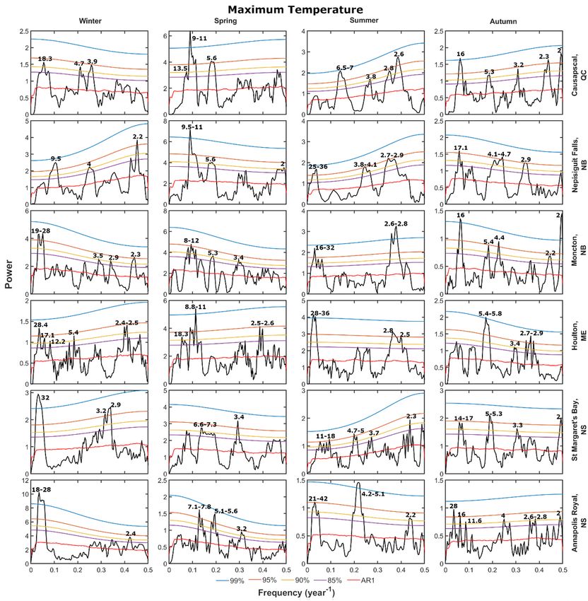
the trend in extreme precipitation in New England was stationary (near–zero linear slope) from 1893–
2005, although some select stations did shown a positive linear trend. In contrast, Frei et al. (2015)
identi ed a pattern of decadal uctuations in the frequency of extreme precipitation events in the
northeastern United States, and an increase in the occurrence of extreme precipitation events during the
warm season (June–October) through the twentieth century. Other studies have reported on general
trends in extreme weather across other parts of eastern North America outside the MR, presenting
evidence of general increases in frequency or intensity of both extreme temperature and extreme
precipitation (Bonsal et al. 2001; Zhang et al. 2001; Vincent et al. 2018; Tan and Gan 2017).

Cyclical Drivers Of Regional Climate Change
Drivers of climate oscillations known to impact weather in eastern North America include the Schwabe
sunspot cycle (SSC, ~11 years), Atlantic Multidecadal Oscillation (AMO, 50–90 years), El Niño Southern
Oscillation (ENSO, 2–10 years), and Quasi–Biennial Oscillation (QBO, 2.1– 2.5 years). The North Atlantic
Oscillation (NAO) and Arctic Oscillation (AO) are also known to in uence eastern North American weather
patterns, though these oscillations do not have well de ned periodicities.

3.1 Sunspot Cycle (SSC)
The SSC, which is characterized by the quasi–periodic rise and fall in the number of observed sunspots,
cycles approximately every 11 years (9–14 year variability in duration; Lassen and Friis-Christensen 1995;
Hathaway 2010, 2015; Jørgensen et al. 2019). Variations in the number of sunspot numbers are related
to changes in total solar irradiance and solar variations have been shown to affect temperatures on both
long and short timescales. Waple et al. (2002) through proxy record analysis demonstrated both long-
and short-term correlations between changes in solar irradiance and global temperature from 1650 –
1850 A.D. A suite of mechanisms control the in uence of solar irradiance on the Earth’s atmosphere,
which can be simpli ed to two main mechanisms: dynamic changes in the troposphere caused by
stratospheric ozone absorption of UV light, and tropospheric heating due to increased solar irradiance
(Gray et al. 2010; Rind et al. 2008; Lockwood 2012).

Earlier studies of North American climate patterns have noted the presence of ~11-year cycles in
temperature and precipitation that have generally been attributed to the in uence of the SSC. For
example, Vines (1984) noted the presence of 9.5 and 11 year cycles in rainfall between 1880 – 1960 in
the Canadian Maritimes. Similarly, Prokoph et al. (2012) recognized an ~11 year cycle in stream ow
records from the St. John River in New Brunswick and the Northeast Margaree River in Nova Scotia.
Currie (1988) noted 10 – 11 year cycles in air temperature in New England, as well as throughout the
continental USA. Currie and O’Brian (1993) observed 10 – 11 year cycles in New England precipitation
records. In fact, the SSC plays a major role in climate variability across the globe. For example, Indian
rainfall totals have indicated moderate correlation with the SSC (Ananthakrishnan and Parthasarathy
1984), and both ~11 and ~22 year cycles (22 years being the double sunspot cycle) have been

                                                  Page 4/36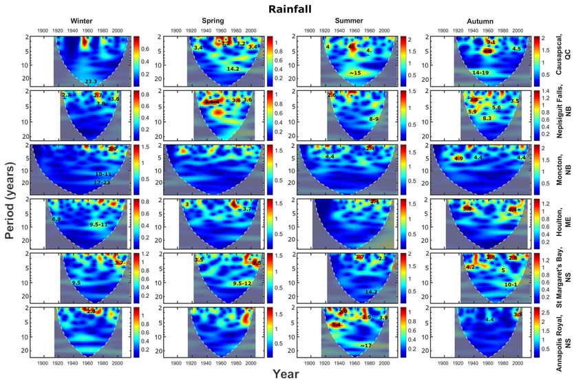
recognized in Indian, African, and Australian precipitation patterns (e.g. Vines 1977, 1980, 1986;
Mazzarella and Palumbo 1992; Currie and Vines 1996; Thresher 2002).

Others have linked the SSC to short term variations in near-surface temperatures in various locations,
though many of these studies have focused on latitudinal zones spread across often vast geographical
distances (van Loon and Shea 1999 2000; van Loon et al. 2004; Meehl and Arblaster 2009; Meehl et al.
2009; Maliniemi et al. 2014). However, the relationship of the SSC to regional variations in temperature
have also been noted in several regional studies, including Romania (Sfîcă et al. 2018), China (Du et al.
2017), and North America (Currie 1993; Mendoza et al. 2001; Mendoza et al. 2006; Nalley et al. 2013).

3.2 Atlantic Multidecadal Oscillation (AMO)
The AMO is an oceanic alternation between warm and cool sea surface temperatures throughout the
Atlantic Ocean, characterized by a quasi-periodic ~64-year cycle (~50-90 year variation) with about 30-35
years per phase (Knudsen et al. 2011). There is evidence that the AMO may be derived from an
oscillatory component in the strength of North Atlantic thermohaline circulation (Dima and Lohmann
2007), which is characterized by a coherent pattern of warm and cold sea surface phases in the North
Atlantic (Schlesinger and Ramankutty 1994). Negative (cold) AMO phases persisted from approximately
1900–1925 and 1965–1995 and positive (warm) phases characterized approximately 1925–1965 and
1995–present (En eld et al. 2001; En eld and Cid-Serrano 2010; Knudsen et al. 2011).

AMO positive phases have been associated with several changes in climate, such as decreased
precipitation, increased temperature, and droughts in North America (En eld et al. 2001; Sutton and
Hodson 2005, 2007; Nigam et al. 2011). However, in reference to extreme temperatures and precipitation,
the AMO has a more prevalent impact on North America by modulating the effects of other climate
phenomena (Mo et al. 2009; Zhang et al. 2012; Kang et al. 2014; Park and Li 2019; Zhang et al. 2019).
When isolated, signi cant in uence of the AMO by itself on North America often exhibits a coastal-inland
gradation (Knight et al. 2006; Patterson and Swindles, 2015). In an analysis of lake ice out records from
Maine and New Brunswick, Patterson and Swindles (2015) recognized signals of not only the 32-year
AMO phase record, but also ~16-year cycles that they attributed to being secondary subharmonics of the
primary AMO multidecadal signal.

3.3 North Atlantic Oscillation (NAO) and Arctic Oscillation
(AO)

                                                  Page 5/36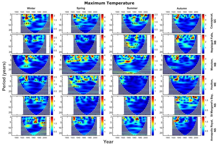
The NAO is a weather phenomenon caused by uctuations in atmospheric pressure at sea–level between
two pressure centers in the North Atlantic; the Azores High and the Icelandic Low. Variation in this
differential pressure in uences the strength and directionality of North Atlantic westerly winds, which in
turn in uences temperature and precipitation patterns in the Atlantic Northern Hemisphere (Hurrell 1995;
Olsen et al. 2012; Patterson and Swindles 2015). The NAO and to a lesser extent AMO have been shown
to have the most signi cant overall impact on winter climate in North America (Burakowski et al. 2010;
Hubeny et al. 2006) The related AO is a measure of broader change in sea–level pressure of Arctic air
masses in the Northern Hemisphere, of which the NAO is a localized constituent of (Deser 2000; Ambaum
et al. 2001; Olsen et al. 2012; Young et al. 2012; Patterson and Swindles 2015). Both the AO and NAO
have similar known in uences on eastern North American weather during their positive (negative) phases,
resulting in typically colder (warmer) temperatures, particularly during winter (Patterson and Swindles
2015; Yang et al. 2020). While both phenomena have relatively poorly de ned frequencies, they typically
range from subdecadal to interdecadal, and are occasionally characterized by 20+ year multidecadal
oscillations (D'Arrigo et al. 2003; Olsen et al. 2012). Steinschneider and Brown (2011), Coleman and
Budikova (2013), and Armstrong et al. (2014) have observed linkages between the NAO and hydroclimate
variations in the eastern North America. Li et al. (2017) correlated intervals of persistent cold spells in
eastern North America to the in uence of the AO. Moreover, the AO is known to be associated with sea ice
formation/melting in the Canadian Arctic (Rigor et al. 2002).

3.4 El Niño-Southern Oscillation (ENSO)
The ENSO originates in the equatorial Paci c where strengthening or weakening of equatorial trade winds
in turn results in a strengthening or weakening of the upwelling of cold deep–ocean waters off the west
coast of South America. This phenomenon has a far-reaching impact, in uencing much of the world’s
climate with both its warm (El Niño) and cool (La Niña) phases (Ropelewski and Halpert 1986; Rodbell et
al. 1999; Moy et al. 2002). In eastern North America, the in uence of the ENSO is the result of the
interaction of various atmospheric teleconnections (Bjerknes 1969; Diaz et al. 2001). Typically, only
strong ENSO phases are re ected in weather patterns in eastern North America, leading to warmer, drier
conditions during El Niño and cooler, wetter (snowier) conditions during La Niña, particularly in winter
(Ropelewski and Halpert 1986; Harrison and Larkin 1998; Wolter et al.1999; Patterson and Swindles 2015;
Yang et al. 2020).

3.5 Quasi-Biennial Oscillation (QBO)
The nal major climate/weather driver considered here is the QBO, which is a measure of the variation
between easterly and westerly winds in the equatorial stratosphere. The QBO record is typically

                                                 Page 6/36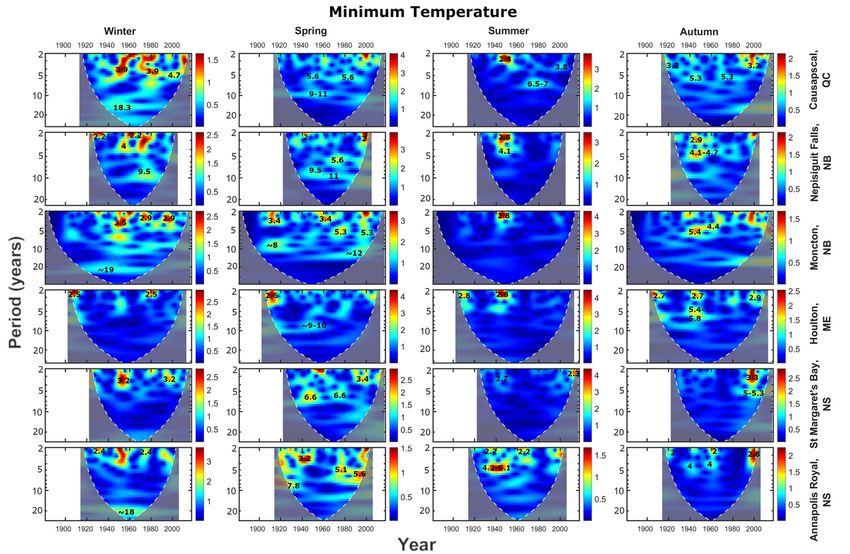
characterized by 2.1-2.2 and 2.3-2.4 year cycles, which have been shown to in uence various aspects of
near-surface climate via polar, subtropical, and tropical teleconnections (Gray et al. 2018). In eastern
North America, the westerly phase of the QBO often leads to cooler surface temperatures, particularly in
winter (Baldwin et al. 2001; Chattopadhyay and Bhatla 2002; Patterson and Swindles 2015). The QBO
has also been shown to impact ice break-up in North American lakes (Sharma and Magnuson, 2014;
Patterson and Swindles, 2015). The timing of lake ice break-up each year is primarily a function of late
winter air temperatures, with other factors such as distance from coast, elevation, wind direction and
wind intensity also being contributing factors (Patterson and Swindles, 2015).

   Interactions between the cycles described above and their resultant in uence on climate are well-
documented. For example, AMO is known to weaken the effects of ENSO, NAO, and AO during its positive
phase and amplify them during its negative phase (Zhang et al. 2012; Kang et al. 2014; Park and Li 2019;
Zhang et al. 2019; Chen et al. 2020). Other climate oscillations thought to in uence weather only weakly
in uence climate in the region, or occur with frequencies of hundreds or thousands of years, well beyond
the instrumental records examined in this study (Mann et al. 1995; Domínguez-Villar et al. 2017).

Methods
4.1       De ning extreme weather
Various methods have been used to record and analyze extreme events (e.g. event counts or incremental
classi cation; statistical, time series, and geospatial analysis; modelling), each tailored to differing
approaches to what de nes an extreme weather event (e.g. severe or unseasonal weather; weather at the
limits of the historical distribution; e.g. Mondal and Mujumdar, 2015; Panda et al., 2016). Phenomena
associated with the broad term “extreme weather event” can include, but are not limited to, rain or
snowstorms, heat waves, cold snaps, droughts, oods, or hurricanes (Meehl et al. 2000; Stephenson et al.
2008; Huber and Gulledge 2011). Thus, a more speci c de nition of extreme weather in the context of
this study is required. A common method for de ning an extreme weather event is a statistical approach
using the 95th percentile of historical climate data collected from a speci c weather station or groups of
stations (Rahmstorf and Coumou 2011; Gao et al. 2012). This concept can be simpli ed mathematically
using the assumption that given aspects of weather (e.g. temperature, precipitation) follow a Gaussian
distribution, with 95% of all weather events falling within two standard deviations of the mean (µ± 2σ,
where µ is the mean and σ is the standard deviation; Frei et al. 2015; Wang et al. 2015). Beyond these two
standard deviations, weather events are considered extreme. This method uses univariate data (e.g. daily
temperature records) and is only suitable for isolated extremes in that data (e.g. one day of abnormally
high temperatures). Here, this method is employed for single day events and is not suitable if one wishes
to recognize longer and/or less isolated events, such as hurricanes, the effects of which can last several
days or weeks. While multi-day events can be recognized and analyzed using this approach, corrections
must be applied to ensure multi-day events are mutually independent (Frei et al. 2015).

                                                 Page 7/36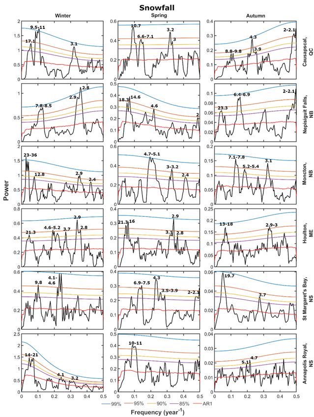
4.2                 Data and analyses
Daily–resolution weather (temperature and precipitation) data was obtained from the historical data
archives of Environment and Climate Change Canada and the National Oceanic and Atmospheric
Association (NOAA) of the United States for 90 weather stations with long high-quality records from
eastern North America (Fig. 1; stations listed in Appendix 1). The raw data spans various date ranges,
typically beginning in the late 19th to early 20th centuries and continuing up to the 2010s, with the latest
year analyzed being 2017. These 90 stations, which were distributed through the provinces of Ontario,
Quebec, New Brunswick, Nova Scotia, and Prince Edward Island, and states of New York, Vermont, New
Hampshire, Maine, Massachusetts, Connecticut, and Rhode Island, were subdivided using hierarchical
agglomerative clustering (Sup. Fig. 1). Cluster analysis took into account the seasonal extreme weather
event totals of each weather variable (maximum temperature, minimum temperature, rain, snow) for each
given location, as well as latitude and longitude, using Ward’s minimum variance linkage (Ward 1963).
 This approach resulted in recognition of three distinct climatic regions (informally designated as the
Continental Region, Central Region, Maritime Region (MR), Sup. Fig. 1), which re ects the diversity of sub-
climates found within this relatively large area of eastern North America.

This study focuses on the MR, which itself comprises distinct climatic subzones that are heavily
in uenced by proximity to the moderating in uence of the Atlantic Ocean. Six stations within the MR
were selected for detailed analysis based on the availability of long-running, high–quality climate records
with no, or negligible missing data. They also provide a wide geographic distribution throughout the MR.
These six locations are St. Margaret’s Bay, NS (1922 – 2018), Annapolis Royal (1915 – 2007), NS,
Moncton, NB (1881 – 2018), Nepisiguit Falls, NB (1922 – 2006), Causapscal, QC (1913 – 2018), and
Houlton, ME (1902 – 2013; Fig. 1).

MATLAB (MathWorks 2019) was used to separate each record by meteorological season (December–
February, March–May, June–August, September–November). The means and standard deviations for
temperature (high, low) and precipitation (snow, rain) were calculated for these four seasons for the
entirety of the available weather records. For precipitation, means and standard deviations were only
calculated for non–zero values, as days with zero precipitation values would unfavourably skew the data.
Temperature and precipitation values that fell outside of two standard deviations from the mean (the
95th percentile) were considered extreme. The number of extreme events for each season and year were
tallied for further analysis.

The variability of extreme weather events through time was analyzed by calculating linear best ts as
well as by red noise spectral and wavelet time series analyses. Spectral and wavelet time series analysis
provide complementary results. Spectral analysis provides a very good estimate of signal periodicity but
presumes stationarity, while non-stationary wavelet analysis provides an indication of the distribution
and interrelationship of signals with varying frequencies through time (Prokoph and Patterson 2004).
Red noise spectral analysis, a function based on Thomson’s multitaper method (Dorothée 2020), was
used to transform time–domain data into its frequency domain counterpart. As opposed to a basic
                                                  Page 8/36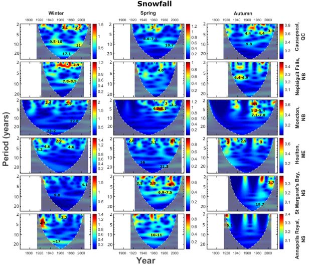
Fourier transform, which provides a single spectral power estimate, this method utilizes several estimates
of a power spectrum and averages them, eliminating potential biases that can arise when using a simple
Fourier transform (Thomson 1982). Red noise and con dence levels were estimated using the Monte
Carlo and chi-square methods (Schulz and Mudelsee 2002). Typically, a 95% con dence interval is used
to validate statistically viable periodic trends, though slightly lower con dence intervals remain
statistically signi cant. Con dence levels of 90% and 99% are also often used in statistical analysis.
Here, any periodic signals above the 90% con dence interval were considered signi cant, as this level still
maintains data robustness (Zar 1998). Continuous wavelet transforms (CWTs) were applied to the
extreme weather records, presenting the spectral information with the additional element of time, which
provides information on the continuous or discontinuous nature of the periodic signals.

Cross wavelet transforms (XWT) were then carried out between the various extreme weather records and
the six climate oscillations discussed in Section 3 (SSC (SILSO, 2021), AMO (Trenberth et al. 2021), AO
(NCAR 2021), NAO (Hurrell and NCAR 2020), ENSO (Trenberth and NCAR 2020) and QBO (NCAR 2013))
using the MATLAB functions by Grinsted et al. (2004), yielding comparisons between the extreme weather
records and climate oscillations. While a CWT is useful to analyze a single time series for oscillatory
components, an XWT can be constructed to reveal the common spectral power between two time series
(i.e. exposing the oscillatory components that both time series share at a given point in time; Grinsted et
al. 2004). This transform is particularly useful for assessing the relationship between two cyclic time
series, providing a visual representation of statistically signi cant correlated oscillations between two
data sets. The XWT scalograms indicate the 95% con dence interval of statistically signi cant common
oscillations (shown as areas of high spectral density outlined with a solid black line). The XWT analyses
were carried out to assess the relationships that the various aspects of extreme weather have to various
climate oscillations.

Results
5.1 Linear regressions
The seasonal linear regressions for each intra-station extreme weather variable are typically characterized
by near-zero to very shallow positive or negative slopes depending on the season and weather variable
(-1.78–0.79 events/100 years; Sup. Fig. 1–4, Sup. Table 1). The shallowness of the slopes and variability
in sign across the region indicates that there has been no consistent, long-term, regional trend in the
periodicity of extreme weather phenomena in the timeframe spanned by the MR instrumental record.
However, there do appear to be several trends in the periodicity of extreme weather events that are unique
to individual or small groupings of climate stations.

In general, there has been an increase in regional seasonal variability of extreme rainfall events with
notably consistent seasonal increases in extreme rainfall events in Houlton, ME and Moncton, NB. There
has also been a consistent increase in extreme snowfall events in Moncton. The remaining stations
display near-zero trends in extreme snowfall.
                                                 Page 9/36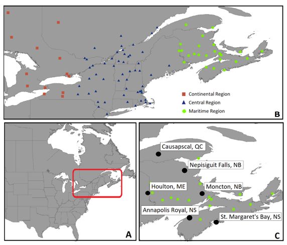
The maximum extreme weather slope observed was 2.37 events/100 years (summer rain, Houlton) and
the minimum observed slope was -4.07 events/100 years (summer minimum temperature, Nepisiguit
Falls, NB). The majority (70.8%) of the linear regressions fall between ‐1 – 1 event/100 years, 85.4% fall
between -1.5 and +1.5 events/100 years, and 90.6% of events fall between -2 and +2 events/ 100 years.
Four of these larger changes were correlated to summer extreme weather records, and three of these
occurred at Nepisiguit Falls, which is characterized by the strongest weather linear trends of any of the
studied stations. Nepisiguit Falls is experiencing declines in both extreme maximum and minimum
temperature events for a given season, indicative of a narrowing of local climate variability (Sup. Fig. 1-4,
Sup. Table 1).
For extreme maximum temperature events the St. Margaret’s Bay, NS, station has been characterized by
consistently positive slopes, whereas the extreme minimum temperatures recorded for the same station
display consistently negative slopes. This step-wise increase in extreme warm temperatures and decrease
in cold temperatures is consistent with a progressively warming local climate at St. Margaret’s Bay.
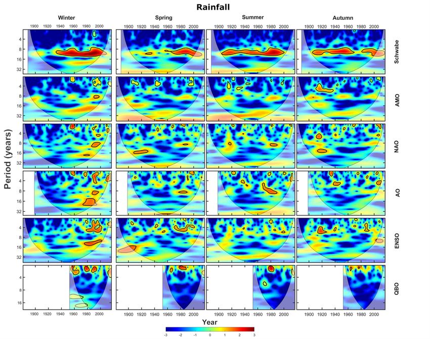
5.2 Spectral analysis and wavelet transforms
Spectral analysis and CWTs display many statistically signi cant cycles at the 90% con dence interval
and higher throughout the MR (Figs. 2–9). Across the six stations, there was variation in the observed
cycles within each of the seasonal weather records, although regional trends and spatial gradients were
observed between stations. Extreme maximum and minimum temperature data exhibited 2.8–3.2 year
non-stationary cycles spanning all the seasons at nearly all stations (Figs. 2–3 and 6–7). This cyclicity is
particularly strong at all stations for 1997–2000 autumn extreme maximum temperature (Fig. 6).
Similarly, a 2.8 year cycle occurred during summer in the mid–1940s at all stations except for St.
Margaret’s Bay and Annapolis Royal, NS. Other cycles in extreme maximum temperature that can be seen
across several, or all stations, are 5.1–6.6 years (spring, 1970s), 9–11 years (spring, 1940–1960), and
3.2–4 years (winter, 1940s). Cycles observed for extreme minimum temperature across nearly all stations
include: ∼3.7 years (autumn, 1980s); 3.2–4.2 years (autumn, 1930s); 2.8–3.3 years (summer, ∼2000);
5.1–5.7 years (spring, ∼1940); and 3.9–5.3 years (winter, 1930s and 1960s).
Most stations are also characterized by statistically signi cant non-stationary extreme rain and snow
precipitation cycles of 2–3 years across all seasons (Figs. 4–5 and 8–9). However, these cycles are not
quite as well correlated across the entire region as was the case for extreme temperature.
There were non-stationary 3.4–3.7 year extreme rainfall cycles (spring, 1990s) observed at all stations,
although this cycle was only statistically signi cant at some stations. There was also a 9.5–11 year non-
stationary cycle (winter, 1970s– 1990s) and ∼3 years (spring, 1910s) observed at Houlton and Moncton.
The records at these two stations also included non-stationary 3.1–3.2 year cycles in extreme snowfall
(spring, ∼2000). There was also a 2–3 year snowfall cycle (autumn, 1950s) present only at St. Margaret’s
Bay and Annapolis Royal.
Page 10/36Regional variation in MR precipitation cycles re ects the in uence of the Atlantic Ocean. The weather at
stations in more coastal environments (St. Margaret’s Bay and Annapolis Royal, NS) typically receive
more precipitation as rainfall throughout the year, as well as being more likely to be impacted by the
remnants of tropical storms than the inland stations. These two coastal stations have similar extreme
precipitation records, quite distinct from the records from the other stations. More inland, continental-
weather-in uenced Houlton and Moncton are also more similar to one another for the same reason.
5.3 Cross wavelet transforms
The XWTs facilitate direct comparison of the documented extreme temperature and precipitation weather
records with the published SSC, AMO, NAO, AO, ENSO, and QBO time series datasets (NCAR 2013, 2020;
Hurrell and NCAR 2020; Trenberth and NCAR 2020; Trenberth et al. 2021; SILSO 2021) by identifying
frequencies that any two time series under investigation (e.g. a regional climate driver and an extreme
weather record) have in common at a given time. The results of the XWT comparison between the SSC,
AMO, NAO, AO, ENSO, and QBO and Annapolis Royal maximum temperature and Moncton rainfall are
presented in Figs. 10 and 11, respectively. These two example climate stations were chosen to highlight
as they are representative of the relationship between these various climate patterns and rainfall and
maximum temperature throughout the entire region. The XWT results between the extreme rainfall,
snowfall, and high and low temperatures for all stations and each of the SSC, AMO, NAO, AO, ENSO, and
QBO phenomena are presented in Sup. Figs. 5–29.
The strongest observed relationship between the extreme temperature and precipitation data and cyclic
climate drivers was an ~ 11 year cycle that correlates with the SSC (Sup. Figs. 5–9). This strong
relationship with the SSC included all stations and all extreme weather types analyzed, and although non-
stationary, in most cases extended throughout the entire instrumental record. Examples of non-
stationarity included a discontinuity between the SSC and maximum temperature in summer (∼1960–
1980) Moncton, Houlton, and St. Margaret’s Bay, as well as during autumn (∼1930–1950 and ∼1970–
1985) in St. Margaret’s Bay and Annapolis Royal. Similar discontinuities were recognized in the SSC-
extreme minimum temperature relationship. The Causapscal, QC, and Nepisiguit Falls stations also
display non-stationarity in the relationships between extreme temperatures and the SSC, though to a
lesser degree. Extreme precipitation shows the highest degree of continuity in common spectral power
with the SSC across the region.
The XWTs for AMO and each of the extreme weather variables (Sup. Figs. 10–13) were characterized by
many small areas of weak common spectral power, although with extreme temperature and precipitation
there was for many stations an area of high common power with a cycle of ∼16–30 years, typically
centered upon ∼1950. This relationship was most apparent with winter and summer maximum
temperature, summer minimum temperature and winter snowfall and was variable by location with
Page 11/36rainfall, appearing most strongly in the coastal stations, St. Margaret’s Bay and Annapolis Royal. Several
occurrences of common ~4 and ~8 year cycles were also observed.
The XWTs for both the NAO (Sup. Figs. 14–17) and AO versus each extreme weather variable (Sup. Figs.
18–21) indicate that these drivers have had a varying impact on extreme high and low temperatures
across the region, with many intermittent occurrences of common cycles ranging from 2 – 16 years. The
climatic in uence of NAO across the region varies considerably between stations, with relatively few, and
typically weak regional patterns. In contrast the XWTs between extreme precipitation and AO indicates
that an abrupt climatic shift occurring around ~1965 for all stations, although prior to this part of the
regional record the common spectral power between extreme precipitation and AO is sparse and weak.
During the post–1965 interval, this relationship became stronger, with higher common spectral power
between the signals. This shift is not as clear when AO is compared to extreme temperatures, though a
clear regional pattern exists. While NAO does not show the time-varying pattern that the AO does, many of
the strongest common cycles between extreme weather and NAO are similar to those shown with the AO.
The ENSO-extreme weather XWT results (Sup. Figs. 22–25) are broadly similar to those patterns
observed for the NAO and AO XWTs. In particular, the XWTs for ENSO and temperature extremes are
strongly correlated between stations, with extreme precipitation showing an abrupt change in common
spectral power beginning in ~1965, as occurred in the AO results. As observed with AO, areas of high
common spectral density increased post–1965, although this trend is less pronounced. The abrupt shift
correlated to ENSO is also apparent across the region with the winter and spring rainfall and spring
snowfall extremes. The high and low frequency signals within the NAO, AO, and ENSO XWTs show
distinct similarities to the resulting AMO XWTs, suggesting a relationship between the effects of these
four phenomena and their in uence on extreme weather.
Each of the ENSO, NAO, and AO versus extreme weather XWTs are also characterized by a relatively
strong 16–30+ year common cycle with various extreme weather records (e.g. winter maximum
temperature – AO, Annapolis Royal (Sup. Fig. 18); summer minimum temperature – NAO, Moncton (Sup.
Fig. 15)), reminiscent of the relationships found between extreme temperature and the AMO. This is most
often found during winter, but these relationships are present in other seasons as well.
The QBO versus extreme weather XWT results (Sup. Figs. 26–29) indicate that this driver has had a
pulsed non-stationary in uence on extreme weather throughout the MR with the most signi cant
in uence being on extreme precipitation, and less so on extreme temperature. The QBO XWT data is
strongly correlated across the region with the notable exception of the Annapolis Royal station. With
extreme maximum temperature, QBO has had a stronger in uence during winter, and has been weakest
during summer. The relationship between QBO and extreme minimum temperature, is fairly uniform
regardless of the season. The most common XWT periodicity observed with temperature has primarily
been in the 2–3 year range, although particularly with extreme maximum temperature there is a semi–
consistent 10–20 year cyclicity that spans from the beginning of the QBO record (1953) to 1980. This 10-
Page 12/3620 cycle is even more strongly expressed with extreme precipitation, with the 2–3 year cycles described
above still present.
Discussion
6.1 Maritime Region (MR) extreme weather trends
Weather patterns in the MR of eastern North America are signi cantly in uenced by its proximity to the
Atlantic Ocean, which moderates the climate there, particularly in coastal areas. However, areas only a
few kilometres inland are signi cantly in uenced by continental climate conditions (Trewartha and Horn
1980; Patterson and Swindles 2015). For example, in summer the Atlantic coast is often shrouded in fog
with temperatures of < 20°C, while it may be sunny and >30°C only a few km inland. Then in winter the
coast may be snow free and rainy while areas only a short distance from the coast may be covered in a
thick blanket of snow. Thus, considering the spatial distribution of weather stations used in this study, a
gradient in climatic trends is fully expected. The gradient in climatic conditions was most signi cant
between the two most coastal weather stations, St. Margaret’s Bay and Annapolis Royal, and the
remaining four stations, which are characterized by more continental climates (e.g. Fig. 7, Sup. Fig. 10).
Of the inland stations the climatic patterns characterizing Moncton and Houlton were most similar to
each other, most likely related to the close latitudinal positioning of the stations at 46.09°N and 46.13°N,
respectively. These results suggest that even at the small regional scale studied, latitudinal climate
gradients impact the periodicity of extreme weather occurrences.
6.2 Linear trends in extreme weather events
Nearly all of the extreme weather records for the MR are, based on regression analysis results,
characterized by fairly shallow slopes, with only relatively small changes, both positive and negative, in
the periodicity of extreme weather through the past ∼100 years, with little spatial coherence. There were
nine weather records in the region though that exceeded an increase/decrease threshold of 2 events/100
years. These records were primarily concentrated in the minimum temperature extremes, particularly for
Nepisiguit Falls and Annapolis Royal (Sup. Table 1). With the vast majority of linear regressions in the
extreme precipitation and temperature records for the MR being negligible through the span of the
instrumental data record examined, the confounding in uence of natural climatic oscillations further
complicate detection of any trajectory in these records. These results, at least for the MR, contrast with
some recently published studies, which report that extreme weather events are becoming more frequent
as global temperatures continue to rise (Perkins-Kirkpatrick et al. 2017; Francis et al. 2018; Keellings et al.
2018; Cowan et al. 2020; Perkins-Kirkpatrick and Lewis 2020).
Page 13/366.3 In uence of Cyclic Climate teleconnections
6.3.1 Schwabe solar cycle (SSC)
The prominent 9–12 year cycles that recurs throughout the extreme weather data for the MR, and the
strong common periodicity in this range between extreme weather and the SSC observed in the XWT
analysis results, indicates that this phenomenon is the most signi cant in uence on each aspect of
climate analyzed in the region (Sup. Fig. 5-9).
The observed linkage between MR extreme weather records to the SSC is similar to the ndings of
Laurenz et al. (2019), where the SSC was found to correlate with European rainfall totals. However, in that
study it was observed that there was a moderate month to month correlation between variation in the
strength of solar in uence on extreme precipitation, which in contrast to the results for the MR, were
signi cantly reduced at the seasonal level. The wider geographic coverage, accompanied by a wider
regional climatic variability, used by Laurenz et al. (2019) may explain the greater month to month
variation between the two studies.
Additionally, Prokoph et al. (2012) attributed an ~11-year cycle in MR steam ow records to the SSC,
although they also noted that this signal was comparably weaker than what was observed in rivers
elsewhere in Canada. Moreover, the SSC is known to in uence other natural cyclic climate phenomena
(e.g. QBO and ENSO (Quiroz 1981; Hamilton 2002; Kuroda 2007; Fischer and Tung 2008; Calvo and
Marsh 2011; Zhou et al. 2013)), which could possibly explain the observed non-stationary relationship
between the SSC and extreme weather in the MR, particularly the relationship with extreme minimum
temperature.
6.3.2 Atlantic Multidecadal Oscillation
The XWTs comparing the AMO index and MR extreme weather data revealed a common ~16–30 year
cycle recognizable in varying degrees in both temperature and precipitation data, which was widespread
across the region between 1930 and 1970. This period range corresponds to a suspected subharmonic
in uence of the AMO on this region; 16-24 year subharmonics of the AMO have been reported by Ruiz-
Barradas et al. (2013) and have been found to in uence climatic trends in the MR, particularly those
related to temperature uctuations, by Patterson and Swindles (2015). Furthermore, this 1930 – 1970
interval, corresponding to a positive phase of the AMO, was most common in extreme temperatures and
snowfall data from Nova Scotia stations, although extreme rainfall data also was characterized by this
pattern, albeit with a weaker spectral power. While this effect was observed most strongly in the Nova
Scotia stations, it appeared more weakly in the remaining MR stations, indicating a coastal-inland effect
of the AMO in this region. This gradational effect can be seen in both extreme temperature/AMO XWTs
Page 14/36(Sup. Figs. 10, 11), in which the coastal Nova Scotia stations experience the strongest relationships,
particularly in winter months.
6.3.3 NAO, AO, and ENSO
Several parallels were observed in the relationships between NAO, AO, and ENSO XWT results. Each of
these oscillations exhibited common cycles of 2–16 years that appeared at similar times between the
three oscillations. Furthermore, both ENSO and AO exhibited a shift from low common spectral power to
high common spectral power at ~1965. These patterns suggest the NAO, AO, and ENSO share an
interactive in uence on extreme weather in the MR.
From the XWT results, both ENSO and AO have a relatively uniform in uence on extreme weather across
the MR, with similar signals observed across all stations for a given season and weather type. In
particular, ENSO has the most signi cant in uence over extreme temperatures in the MR, particularly in
winter and spring (Sup. Fig. 22-23). ENSO and AO collectively have a similar but more moderate in uence
on extreme precipitation (Sup. Fig. 24-25, Sup. Fig. 20-21), with the NAO having a comparatively weaker
in uence on this parameter. In contrast to ENSO and AO, the in uence of the NAO often has a higher
spatial variation with respect to extreme weather throughout the MR (Sup. Fig. 14-17).
There is a notable common 16–30 year cycle observed in the XWT extreme temperature records for the
NAO, AO, and ENSO, particularly during winter. These lower frequency cycles parallel similar XWT results
observed with the AMO data. In addition, ~4 and ~8 year XWT links between the AMO and extreme
weather records also parallel many of the signi cant relationships observed with the XWT derived
correlations between extreme weather and ENSO, NAO, and AO. These resemblances suggest a strong
interaction and signi cant modulation of ENSO, NAO, and AO by the AMO in the MR (e.g. Fig. 10 displays
stark similarities between the maximum temperature XWT analyses for AMO, NAO, AO, and ENSO at
Annapolis Royal, NS).
The interrelationship between AMO, NAO, AO, and ENSO is particularly strong in coastal areas, particularly
in the respective extreme temperature XWTs. For example, the extreme maximum temperature record
from Annapolis Royal record is characterized by a close similarity observed within each season between
each of these four climate oscillations (Fig. 10). This close relationship between these oscillations is
also observed at many inland stations, albeit generally less strongly (e.g. Moncton extreme rainfall, Fig.
11). This same pattern is also weakly observable in the extreme precipitation XWTs, although it is much
more variable.
In the MR, this in uence was further supported by observed patterns within the AO–extreme precipitation
XWTs. For example, the common periodicity between AO and extreme precipitation became ampli ed
after 1965 following the establishment of an AMO- phase. A similar post–1965 ampli cation was
Page 15/36observed in the ENSO XWT record, although these effects were more varied by season and weather type.
The signi cant in uence of the AMO in modulating the effects of other cyclic climate phenomena (such
as the NAO, AO, and ENSO) has also been previously documented elsewhere in North America, where it
has been observed that this phenomenon suppresses the in uence of their effects during an AMO+ phase
and amplifying them during an AMO- phase (Mo et al. 2009; Zhang et al. 2012; Kang et al. 2014; Park and
Li 2019; Zhang et al. 2019).
6.3.4 The Quasi-Biennial Oscillation
In the MR the in uence of the QBO appeared strongest within the extreme precipitation record (both rain
and snow) and was weakest within the extreme minimum temperature record. This result is partially
contradictory to the spectral analysis results, where 2–3 year cycles appeared in nearly all extreme
temperature records and, less commonly in the extreme precipitation records. A possible explanation for
the discrepancy is that there is probable overlap between lower frequency QBO and higher frequency
ENSO signals. This strong observed correlation between QBO and uctuations in extreme rainfall and
snowfall patterns is also supported by research from elsewhere in North America and around the globe
(Lau and Sheu, 1988; Brázdil Zolotokrylin 1995; Inoue and Yamakawa 2010; Seo et al. 2013). Similarly,
several extreme rainfall records have been found to be characterized by quasi-biennial patterns, although
in many cases they have not necessarily being linked to the QBO (Nastos and Zerefos 2007; Becker et al.
2008; Han et al. 2020).
The lower–frequency cycles observed in many of the QBO XWTs from 1953–1980 (e.g. Fig. 10, QBO row)
are likely a result of modulation of what has been dubbed the quasi–decadal oscillation, which has been
attributed to in uence of the SSC (e.g. Quiroz,1981; Hamilton, 2002; Fischer and Tung, 2008). It is
hypothesized that changes in TSI through the 11-year SSC in uences movement of upper stratospheric
air masses, where there are also strong SSC-linked changes in solar–ozone radiative forcing.
Overprinting on the QBO signal results in a quasi–decadal trend within in the QBO index. In the MR this
modulation is seen most strongly in the pre-early 1980s QBO.
Conclusions
Through implementation of spectral, Morlet wavelet and cross wavelet analysis we have demonstrated
that the occurrence of extreme weather (precipitation (snow, rain) and temperature (high, low)) in the
instrumental record (~100-150 years) from six climate stations in the MR of eastern North America is
largely cyclical, showing only localized evidence of either negative or positive trends. A regional gradation
in extreme weather occurrence is recognizable when comparing coastal and inland/continental areas. It
was found that the observed cyclic components of seasonal extreme weather are principally driven by
several natural climate oscillations, the strongest of which is the ~11-year SSC. The SSC cycle exhibited
Page 16/36both continuous and discontinuous impact through time in all seasons on the occurrence of extreme
maximum and minimum temperature, rainfall, and snowfall.
Other cycles found to in uence the occurrence of extreme weather were the AMO, NAO, AO, ENSO, and
QBO. The in uence of NAO, AO, and ENSO on extreme weather were modulated by negative and positive
phases of the AMO, with distinct similarities between the four oscillations that would otherwise be
unexpected. In particular the negative phase of the AMO appears to amplify the impacts of the AO and
ENSO. Moreover, comparison of the AMO, NAO, AO, and ENSO records with extreme weather records in the
MR indicates that there seems to be a complex interplay between them that causes some uniformity in
their in uence, particularly on extreme temperature events through the 20th and early 21st centuries for a
given station.
The QBO had a frequent but discontinuous impact on extreme weather in the MR through time,
having a stronger relationship with extreme precipitation than extreme temperature. Furthermore, there
was a modulating effect of the SSC on the QBO spanning from the 1950s to the 1980s, which was
re ected in the XWT analysis for most stations in the MR.
References
Ambaum, M. H., Hoskins, B. J., and Stephenson, D. B. (2001). Arctic oscillation or North Atlantic
oscillation? J Clim, 14(16):3495–3507.
Ananthakrishnan, R. and Parthasarathy, B. (1984). Indian rainfall in relation to the sunspot cycle: 1871–
1978. J Climatol, 4(2):149–169.
Andalo, C., Beaulieu, J., and Bousquet, J. (2005). The impact of climate change on growth of local white
spruce populations in Quebec, Canada. For Ecol Manag, 205(1-3):169–182.
Andrey, J., Mills, B., Leahy, M., and Suggett, J. (2003). Weather as a chronic hazard for road transportation
in Canadian cities. Nat Hazards, 28(2-3):319–343.
Armstrong, W. H., Collins, M. J., and Snyder, N. P. (2014). Hydroclimatic ood trends in the northeastern
United States and linkages with large-scale atmospheric circulation patterns. Hydrol Sci J, 59(9):1636–
1655.
Balbus, J. M. and Malina, C. (2009). Identifying vulnerable subpopulations for climate change health
effects in the United States. J Occup Environ Med, 51(1):33–37.
Baldwin, M., Gray, L., Dunkerton, T., Hamilton, K., Haynes, P., Randel, W., Holton, J., Alexander, M., Hirota, I.,
Horinouchi, T., et al. (2001). The quasi-biennial oscillation. Rev Geophys, 39(2):179–229.
Becker, S., Hartmann, H., Coulibaly, M., Zhang, Q., and Jiang, T. (2008). Quasi periodicities of extreme
precipitation events in the Yangtze River basin, China. Theor Appl Climatol, 94(3-4):139–152.
Page 17/36Bjerknes, J. (1969). Atmospheric teleconnections from the equatorial Paci c. Mon Weather Rev,
97(3):163–172.
Boland, G., Melzer, M., Hopkin, A., Higgins, V., and Nassuth, A. (2004). Climate change and plant diseases
in Ontario. Can J Plant Pathol, 26(3):335–350.
Bonsal, B. and Shabbar, A. (2011). Large-scale climate oscillations in uencing Canada, 1900-2008.
Canadian Councils of Resource Ministers.
Bonsal, B., Zhang, X., Vincent, L., and Hogg, W. (2001). Characteristics of daily and extreme temperatures
over Canada. J Clim, 14(9):1959-1976.
Bouwer, L.M., 2019. Observed and projected impacts from extreme weather events: implications for loss
and damage. In Loss and damage from climate change (pp. 63-82). Springer, Cham.
Brázdil, R. and Zolotokrylin, A. (1995). The QBO signal in monthly precipitation elds over Europe. Theor
Appl Climatol, 51(1-2):3–12.
Burakowski EA, Braswell RH, Wake CP, Bradbury J, Brown DP (2010) In uence of NAO, ENSO, and AMO on
northeast US winter temperatures and snow cover: 1949–2005. Carbon Solutions New England report, p
12
Calvo, N. and Marsh, D. R. (2011). The combined effects of ENSO and the 11 year solar cycle on the
Northern Hemisphere polar stratosphere. J Geophys Res: Atmos, 116(D23).
Chattopadhyay, J. and Bhatla, R. (2002). Possible in uence of QBO on teleconnections relating Indian
summer monsoon rainfall and sea-surface temperature anomalies across the equatorial paci c. Int J
Clim, 22(1):121–127.
Chen, S., Chen, W., Wu, R., and Song, L. (2020). Impacts of the Atlantic Multidecadal Oscillation on the
spring Arctic Oscillation-following East Asian summer monsoon relation. J Clim.
Cheng, C. S., Auld, H., Li, Q., and Li, G. (2012). Possible impacts of climate change on extreme weather
events at local scale in south–central Canada. Clim Change, 112(3-4):963–979.
Cohen, J., Screen, J. A., Furtado, J. C., Barlow, M., Whittleston, D., Coumou, D., Francis, J., Dethloff, K.,
Entekhabi, D., Overland, J., et al. (2014). Recent Arctic ampli cation and extreme mid-latitude weather.
Nature Geosci, 7(9):627.
Coleman, J. S. and Budikova, D. (2013). Eastern US summer stream ow during extreme phases of the
North Atlantic Oscillation. J Geophys Res: Atmos, 118(10):4181–4193.
Cowan, T., Undorf, S., Hegerl, G. C., Harrington, L. J., and Otto, F. E. (2020). Present day greenhouse gases
could cause more frequent and longer Dust Bowl heatwaves. Nature Clim Change, pages 1–6.
Page 18/36Currie, R. G. (1993). Luni-solar 18.6-and solar cycle 10–11-year signals in USA air temperature records. Int
J Clim, 13(1):31–50.
Currie, R. G. and O’Brien, D. P. (1988). Periodic 18.6-year and cyclic 10 to 11 year signals in northeastern
United States precipitation data. J Climatol, 8(3):255–281.
Currie, R. G. and Vines, R. G. (1996). Evidence for luni–solar and solar cycle signals in Australian rainfall
data. Int J Clim, 16(11):1243–1265.
D’Arrigo, R. D., Cook, E. R., Mann, M. E., and Jacoby, G. C. (2003). Tree-ring reconstructions of temperature
and sea-level pressure variability associated with the warm-season Arctic Oscillation since AD 1650.
Geophys Res Lett, 30(11).
Deser, C. (2000). On the teleconnectivity of the “Arctic Oscillation”. Geophys Res Lett, 27(6):779–782.
Diaz, H. F., Hoerling, M. P., and Eischeid, J. K. (2001). ENSO variability, teleconnections and climate
change. Int J Clim, 21(15):1845–1862.
Dima, M. and Lohmann, G. (2007). A hemispheric mechanism for the Atlantic Multidecadal Oscillation. J
Clim, 20(11):2706–2719.
Dolney, T. J. and Sheridan, S. C. (2006). The relationship between extreme heat and ambulance response
calls for the city of Toronto, Ontario, Canada. Environ Res, 101(1):94–103.
Domínguez-Villar, D., Wang, X., Krklec, K., Cheng, H., & Edwards, R. L. (2017). The control of the tropical
North Atlantic on Holocene millennial climate oscillations. Geology, 45(4), 303-306.
Dorothée (2020). Red Noise Con dence Levels (https://www.mathworks.com/
matlabcentral/ leexchange/45539-rednoise_con dencelevels). MATLAB Central File Exchange, retrieved
February 11, 2020.
Douglas, E. M. and Fairbank, C. A. (2010). Is precipitation in northern New England becoming more
extreme? Statistical analysis of extreme rainfall in Massachusetts, New Hampshire, and Maine and
updated estimates of the 100-year storm. J Hydrol Eng, 16(3):203–217.
Du, J., Wang, K., Wang, J., and Ma, Q. (2017). Contributions of surface solar radiation and precipitation to
the spatiotemporal patterns of surface and air warming in China from 1960 to 2003. Atmos Chem Phys,
17(8).
En eld, D. B. and Cid-Serrano, L. (2010). Secular and multidecadal warmings in the North Atlantic and
their relationships with major hurricane activity. Int J Clim, 30(2):174– 184.
En eld, D. B., Mestas-Nun˜ez, A. M., and Trimble, P. J. (2001). The Atlantic Multidecadal Oscillation and
its relation to rainfall and river ows in the continental us. Geophys Res Lett, 28(10):2077–2080.
Page 19/36Fischer, P. and Tung, K. (2008). A re-examination of the QBO period modulation by the solar cycle. J
Geophys Res: Atmos, 113(D7).
Francis, J., Ski c, N., and Vavrus, S. (2018). North American weather regimes are becoming more
persistent: Is Arctic ampli cation a factor? Geophys Res Lett, 45(20):11–414.
Frei, A., Kunkel, K. E., and Matonse, A. (2015). The seasonal nature of extreme hydrological events in the
northeastern United States. J Hydrometeorol, 16(5):2065–2085.
Gao, Y., Fu, J. S., Drake, J., Liu, Y., and Lamarque, J.-F. (2012). Projected changes of extreme weather
events in the eastern United States based on a high resolution climate modeling system. Environ Res Lett,
7(4):044025.
Gray, L.J., Beer J., Geller, M., Haigh, J.D., Lockwood, M., Matthes, K., Cubasch, U., Fleitmann, D., Harrison,
G., Hood, L., Luterbacher, J., Meehl, G.A., Shindell, D., van Geel, B. White, W. (2010). Solar in uences on
climate. Rev Geophys, 48:RG4001.
Gray, L. J., Anstey, J. A., Kawatani, Y., Lu, H., Osprey, S., and Schenzinger, V. (2018). Surface impacts of the
Quasi Biennial Oscillation. Atmos Chem Phys, 18(11):8227–8247.
Grinsted, A., Moore, J. C., and Jevrejeva, S. (2004). Application of the cross wavelet transform and
wavelet coherence to geophysical time series. Nonlinear Proc Geophys, 11(5/6):561–566.
Hamilton, K. (2002). On the quasi-decadal modulation of the stratospheric QBO period. J Clim,
15(17):2562–2565.
Hathaway, D. H. (2010). The Solar Cycle. Living Rev Sol Phys, 7(1):2367– 3648.
Han, T., Li, S., Hao, X., and Guo, X. (2020). A statistical prediction model for summer extreme precipitation
days over the northern central China. Int J Clim, 40(9):4189–4202.
Harrison, D. and Larkin, N. (1998). Seasonal US temperature and precipitation anomalies associated with
El Nin˜o: Historical results and comparison with 1997-98. Geophys Res Lett, 25(21):3959–3962.
Hathaway, D. H. (2015). The Solar Cycle. Living Rev Sol Phys, 12(1):4.
Hubeny JB, King JW, Santos A (2006) Subdecadal to multidecadal cycles of Late Holocene North Atlantic
climate variability preserved by estuarine fossil pigments. Geology 34:569–572
Huber, D. G. and Gulledge, J. (2011). Extreme weather and climate change: Understanding the link,
managing the risk. Pew Center on Global Climate Change Arlington.
Hurrell, J. W. (1995). Decadal trends in the North Atlantic Oscillation: regional temperatures and
precipitation. Science, 269(5224):676–679.
Page 20/36You can also read