Path Optimization for Ground Vehicles in Off-Road Terrain
←
→
Page content transcription
If your browser does not render page correctly, please read the page content below
Path Optimization for Ground Vehicles in Off-Road Terrain
                                                                                     Timothy Overbye and Srikanth Saripalli

                                           Abstract— We present a method for path optimization for
                                        ground vehicles in off-road environments at high speeds. This
                                        path optimization considers the kinematic constraints of the
                                        vehicle. By thinking in the actuator space we can represent these
                                        constraints as limits in the space rather than derived properties
                                        of the path. In this paper we present a actuator space approach
                                        to path optimization for off-road ground vehicles. This is done
arXiv:2101.00769v1 [cs.RO] 4 Jan 2021

                                        by representing and operation on the path as a list of steering
                                        angles over the path length. This transforms the set of kinematic
                                        constraints into constraints on the steering angle. We then put
                                        this path into a gradient descent solver. This produced paths
                                        that are kinematically feasible and optimized in accordance                         Fig. 1.   The Warthog with attached sensors.
                                        with our cost function. Finally, we tested the system both in
                                        simulation and on an off-road vehicle at speeds of 5 m/s.

                                                             I. INTRODUCTION                                    latency multiplied by the vehicle speed. Since path planning
                                                                                                                (along with sensor segmentation) takes up the bulk of this
                                           High speed navigation requires paths that can be generated           time, this radius can be significantly reduced by improved
                                        quickly, satisfy the constraints of the vehicle, and avoid              planning methods. The ideal situation is a planner that is
                                        collision. Unfortunately, the quality of the resulting path and         both fast and satisfies all constraints. However, this is hard
                                        the time to compute the path are often inversely related.               to achieve [1][2]. Another solution is to take a quickly
                                        To solve this issue hierarchical planners are often used that           generated path and apply constraints after generation through
                                        have shorter, but higher fidelity, trajectories at the lowest           an optimization process. By doing this you can gain some of
                                        level. However, if the higher level paths contain infeasable            the benefits of both fast and accurate planners. Although it
                                        paths then these lower level trajectories can easily get stuck.         should be noted that the constraints may significantly change
                                        Therefore, we want a method to take these higher level                  the optimal path such that a path optimizer, if given this
                                        paths and improve their feasibility before they’re passed to            initial path, will converge to some locally optimal path rather
                                        the lower levels. Since a large challenge to feasibility is             than the global optimal. Thus, a distinction should be made
                                        kinematic constraints it makes sense to transform the path to           between an optimized path and an optimal path.
                                        a representation that makes these constraints easy to satisfy.
                                        Here we use the actuator space representation. That is, rather
                                                                                                                B. Actuator Space Representation
                                        than represent the path as a list of vehicle states we instead
                                        represent the path as a list of control inputs. The trade-off              As vehicle speed increases the kinematic, and even dy-
                                        is an increase in complexity of world space constraints such            namic, constraints can restrict the free space of the vehi-
                                        as obstacles.                                                           cle even more than the physical obstacles present in the
                                           In this paper we propose a path optimization framework               environment. Therefore, it becomes advantageous to start
                                        in this actuator space for ground vehicles. By optimizing the           thinking in a framework where these constraints can be
                                        higher level path additional constraints can be applied to it           nativity represented. Typical world space representation are
                                        after generation. Next we will discuss the benefits of both             good at representing obstacles but have no native way to rep-
                                        optimization and the actuator space representation in more              resent kinematic constraints such minimum turning radius.
                                        detail.                                                                 Additionally, path properties like smoothness are harder to
                                                                                                                quantify.
                                        A. Path Optimization
                                                                                                                   Representing the path in the actuator space switches this
                                           Many methods to get optimal paths that satisfy all con-              problem around. Now, provided with a good vehicle model,
                                        straints are slow. This is important due to the relationship            kinematic and smoothness constraints can be represented
                                        between processing rate, vehicle speed, and the minimum                 as obstacles in the actuator space. However, as vehicles
                                        reaction radius. The minimum reaction radius is the mini-               inevitably operate in the real world, and typically aren’t
                                        mum distance at which the vehicle is capable of reacting to             interested in purely achieving some actuator state, we must
                                        new information. It can be thought of as the total system               still consider the world space. Thus, requiring us to trans-
                                          1 Timothy Overbye and Srikanth Saripalli are with the Department of
                                                                                                                form between representations when checking for obstacles.
                                        Mechanical Engineering, Texas A&M University, College Station, TX       This leads to a trade-off between the ease of representing
                                        77840, USA overbye2@tamu.edu ssaripalli@tamu.edu                        kinematic constraints and world constraints.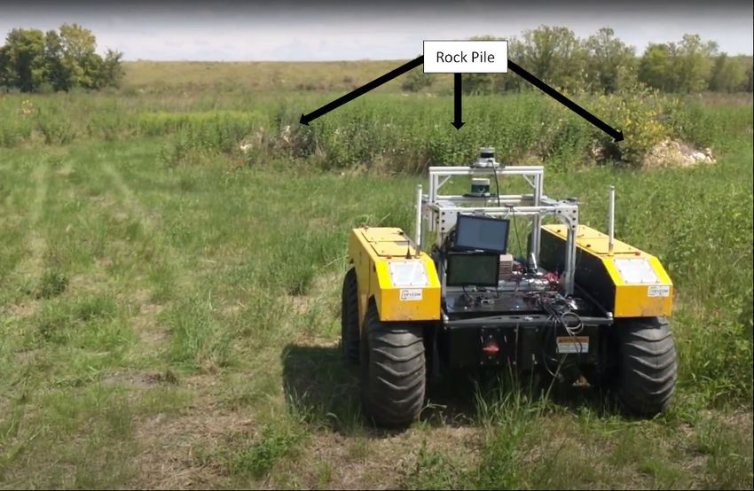
II. RELATED WORK                                such as max steering angle and max steering angle rate
   There have been many works published on the path                are natural to the path formulation[18]. However, there is
planning and optimization problem. Here, we will review            no closed form solution to the clothoid path. Additionally,
some of them as they pertain to some related domains.              clothoids can only represent a subset of all feasible paths.
                                                                   Most recent optimization work has represented the paths
A. Manipulators                                                    as polynomial splines [19][20][21][22]. These splines trade
   This concept of actuator space planning has a long history      some of the benefits of clothoids for the closed form nature of
in manipulator planning. In fact, it’s typical for manipulator     polynomials. Additionally, they can represent a much larger
planning to be done entirely within the actuator space with        segment of the set of all feasible paths.
obstacles transformed into it from the world space. However,
                                                                                             III. APPROACH
manipulators have the advantage that their actuator space and
state space are identical. Typically, they are trying to achieve      Our approach to this problem can be divided into three
given state in the actuator space so, aside from the initial       main stages as shown in figure 2. First is costmap and base
obstacle transform, transforming states isn’t necessary. This      path generation. Here sensor data is fused into a costmap and
leads to an ideal environment for optimization with several        an initial path is made over the map. Next in the optimizer
works being done [3][4][5].                                        this path is fist transformed into the actuator space. The
                                                                   path is put into an iterative gradient descent solver until
B. Air Vehicles                                                    either a minimum cost is achieved or a maximum number
   Recently, the concept of actuator space has had some            of iterations is reached. Finally, we reach the speed control
applications in planning for air vehicles, typically small         section where the resulting path is put through a speed
quadcoptor Unmanned Air Systems (UAS). However, this               controller assigning each point along the path a target speed.
transform will often only be used to check that the path is
within the limits of the actuator[6][7]. Due to the kinematics
of these UAS, scaling the path speed around offending
segments is typically all that’s needed to satisfy these con-
straints. So the path can be transformed into the actuator
space and rescaled without the need to directly plan in the
space.
   From an optimization point of view, UAS are another
good candidate for path optimization [8][9]. They typically
operate in binary space, that is, the space is either free or
has an obstacle and there is no preference for one set of free
space over another. Additionally, due to their higher speed,
path smoothness is highly desired. Thus making kinematic
constraints the dominating factor in path planning.
C. Ground Vehicles
   For ground vehicles, thinking in the actuator space isn’t
a new idea. Model predictive control can be thought of as
operating in this context. Additionally, many methods of
trajectory sampling or path primitive generation fall into this
context. However, due to the larger set of constraints on
ground vehicles and the comparatively complex set of world
space obstacles, longer path planning is typically done in
the world space. Although there have been some examples
of actuator space planning for short trajectories [10].
   Optimization has also seen comparatively less literature
than in the other domains. Most of what exists is used
as a path smoother for planners such as the RRT fam-
                                                                   Fig. 2. Optimizer architecture. From the top, sensor and position data is
ily [11]. The history of path optimizers can be thought            used to make the costmap and base path. In the middle is the path optimizer.
of as beginning with the application of Dubins [12] (and           Finally, the speed controller at the bottom
later Reed-Sheep’s paths) to methods such as A* [13][14]
and it’s derivatives, such as D* [15] and D* Lite [16],
and RRT [17]. Although these paths can be thought of as            A. Cost Map Creation
satisfying all the kinematic constraints they are discontinuous      The cost map process is a continuation on the methods
in steering angle. A solution to this is the clothoid path.        developed in [23]. A lidar scan is taken over a local grid
Clothoid guarantee continuous steering angle and limits            map. From this scan, obstacles are extracted by taking the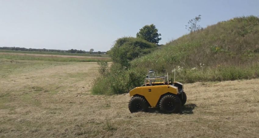
heigh difference between the minimum and maximum height                        chosen due to its guarantee of optimality and fast run time.
return in each cell. If this difference is larger than a given                 Here, we used 8 way connectivity and the euclidean distance
threshold then the cell is marked as containing an obstacle.                   as a heuristic. The vehicle’s current position is used as the
Here, we consider two types of obstacles, hard obstacles                       start of the search. If the goal point is within the local map
(trees, rocks, people, etc) are those that should never be                     it is used as the goal for A*. Otherwise, the closest point
driven through, and soft obstacles (bushes, tall grass, etc) that              within the map to the goal is used for A*. This search is
should be avoided but are traversable. This is determined by                   done over the same costmap as the optimization. Despite the
our segmentation layer, each lidar return is marked as either                  guarantee of optimality of A* it doesn’t take into account the
a hard or soft object. If there are soft object returns above                  kinematic constraints of the vehicle. Thus the final optimized
the obstacle threshold but no hard returns then the cell is a                  path will deviate from the A* path.
soft obstacle. Otherwise, if there’s a hard return above the
threshold it’s a hard obstacle.                                                C. Path Representation
   Both the hard and soft obstacle maps share a common                            Once the base path is generated it needs to be converted
process, shown in figure 3. As they are binary maps, rather                    into the actuator space. The typical path representation in
than a continuous function, they can be expanded with a                        the world space is a list of (x, y, θ) representing the position
dilate operation by the radius of the robot. The area inside                   and orientation of the vehicle on a 2D plane. An actuator
this expanded region is then converted into a distance region.                 space path is represented by a list of (φ, dr) along with the
Where the value of each pixel represents the distance to                       initial (x0 , y0 , θ0 ). Here φ is the current steering angle and
the edge of the region. This is done to ensure that there                      dr is the distance traveled over some fixed time step. We
is always a strong gradient in the costmap to push the                         assume a constant path speed. Figure 4 shows an example
solution out of obstacles. Finally, a similar process is done                  path represented in both world and actuator space.
to create a repulsive halo around around obstacles. This,
once again, helps the solver avoid obstacles but also prevents
discontinuities in the cost map.

                                                                               Fig. 4. A path around a square obstacle represented in both world space
                                                                               (top) and actuator space (bottom).

                                                                                  To convert the path from world space to actuator space
Fig. 3. Cost map formulation. Top, a sample segmented lidar scan with          we need to have an inverse model of the vehicle. Note that
hard obstacles in pink, soft obstacles in red, and ground in green. Middle     this method isn’t tied to a particular model but does require
left, the input map with hard obstacles in black, soft obstacles in grey,
and free space in white. The expanded hard and soft obstacle maps (center      an inverse model. Here we use a 2D model although a 3D
middle ,center right). The cost gradients associated with both obstacle maps   model could be used at the cost of increased dimensionality.
(bottom middle ,bottom right). Finally, the combined cost map (bottom left).   Equations 1 and 2 describe the inverse model. If the input
                                                                               path doesn’t contain heading information then we can use
   The final costmap is the simple per-pixel sum of both of                    equation 3 to back calculate it. Although this will leave the
these sub-maps. Thus, we maintains both the strong gradients                   heading at the final point undefined, in practice it can be
and continuity in the final costmap.                                           assumed to be the same as that of the next to last point.
B. Base Path Generation
                                                                                                   φi = θi+1 − θi                                 (1)
  Before the optimizer can run it needs to be given a base                                      p
path. For our implementation we chose to use A* [13]. It was                                dr = (xi+1 − xi )2 + (yi+1 − yi )2                    (2)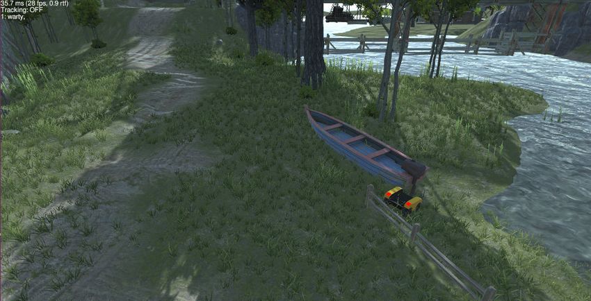
θi = arctan(yi+1 − yi , xi+1 − xi )                        (3)   E. Path Solver
  Transforming from the actuator space to world space is                         With the cost function now defined the path can be sent to
easier. It can be thought of as simply integrating the for-                   the solver. Here, we cause perturbations to the path at each
ward model with respect to some starting point (x0 , y0 , θ0 ).               point such that each perturbation decreases the cost of the
Equations 4, 5, and 6 describe this process.                                  path. However, perturbations at the start of the path will have
                                                                              a much larger total effect on the path than perturbations later
                             θi+1 = θi + φi                             (4)   in the path. Additionally, the actuator space does not fix the
                                                                              goal point of the path. To solve both these issues we dampen
                      xi+1 = xi + cos(θi )dr                            (5)
                                                                              the perturbation over the next N time steps. This is done by
                         yi+1 = yi + sin(θi )dr                         (6)   using an S curve to interpolate between the perturb path and
D. Cost Function Formulation                                                  the original path in world space then transforming this path
                                                                              back into actuator space. Figure 5 shows this process for
   Finally, we define the cost function to optimize against
                                                                              a perturbation at step 5 with a damping length of 25 time
(equation 7). Here P represents the path and p is a point in
                                                                              steps.
the path. We have already talked about the costmap but to
                                                                                 The solver itself is a simple implementation of gradient
fully capture the cost of a path we must also consider it’s
                                                                              descent. It is described by algorithm 1. In brief, the cost
kinematic properties. This leads to a cost function with both
                                                                              for the perturbed segment is checked for both left and right
a map cost and a kinematic cost.
                                                                              perturbations over the perturbation distance. This, along with
                                                                              the current cost of that segment, defines the gradient. Then,
                 F (P ) = Fmap (P ) + Fpath (P )                        (7)
                                                                              a final perturbation is chosen for that point according to
  Breaking down this function further leads to the next two                   the gradient and a scaling factor. This process is repeated
equations. The costmap cost (equation 8) is simply the sum                    for each point along the path. When there exist no more
of all the cost map cells through which the path moves.                       cost reducing perturbations along the path, or the maximum
                                    P                                         iteration limit is reached, the path is returned.
                                    X
                 Fmap (P ) =              M ap[px , py ]                (8)
                                      p                                       Algorithm 1 Optimizer
   Next, we are concerned with the constraints imposed on                      1: currentCost = Cost(path)
the vehicle by our kinematic model. Here we get two main                       2: lastCost = inf
constraints on the path, the steering angle φ must lie between                 3: while currentCost < lastCost do
some maximum and minimum values (equation 9). Typically,                       4:    lastCost = currentCost
we can assume that −φmin = φmax so this constraint                             5:    for point in path do
reduces to equation 10.                                                        6:      costlef t = Cost(P erturb(point, lef t))
                                                                               7:      costright = Cost(P erturb(point, right))
                          φmin ≤ φ ≤ φmax                               (9)    8:      if costlef t < currentCost then
                                                                               9:         scale = currentCost − costlef t
                               |φ| ≤ φmax                              (10)   10:         path = P erturb(point, lef t ∗ scale)
  Similarly, the rate of change in the steering angle is also                 11:         currentCost = Cost(path)
of interest to us. This leads to another set of constraints in                12:      end if
equation 11 . Once again we can assume that −φ̇min = φ̇max                    13:      if costright < currentCost then
so this constraint reduces to equation 12.                                    14:         scale = currentCost − costright
                                                                              15:         path = P erturb(point, right ∗ scale)
                          φ̇min ≤ φ̇ ≤ φ̇max                           (11)   16:         currentCost = Cost(path)
                               |φ̇| ≤ φ̇max                            (12)   17:      end if
                                                                              18:    end for
  Rather than writing these as hard constraints, we instead                   19: end while
represent them by large, steep cost gradients outside of the                  20: return path
boundaries. However, even within the boundaries imposed
by our constraints we are still interested in smooth paths.
Equation 13 is the final kinematic cost function with α, β                    F. Speed Control
being the in and out of bounds cost factors respectively.
                                                                                 So far we have only been concerned with the steering
                   P                                                          angle of the vehicle and any obstacles the path might run
                   X
    Fpath (P ) =          (f (pφ , αφ , βφ ) + f (pφ̇ , αφ̇ , βφ̇ ))   (13)   into. However, we also want the vehicle to traverse this path
                     p                                                        as fast as possible. Thus the need for a speed planner that
                 (                                                            will maintain a high speed while respecting the constraints
                     α|φ|,                   if |φ| < φmax                    of the vehicle. Speed control is done in two passes. First, the
 f (φ, α, β) =
                     αφmax + β(|φ| − φmax ), otherwise                        maximum speed at each point is determined based on that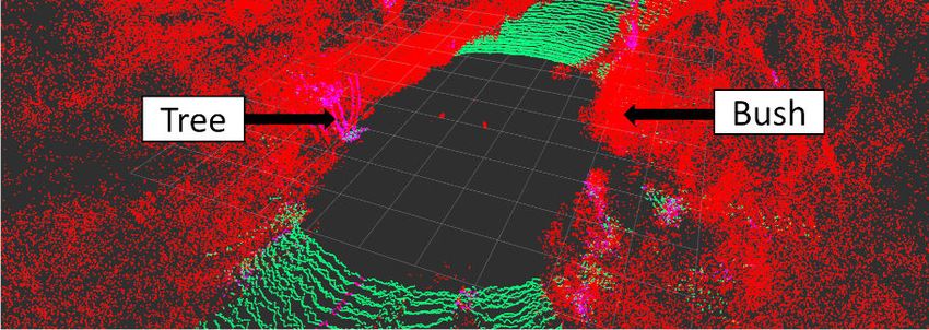
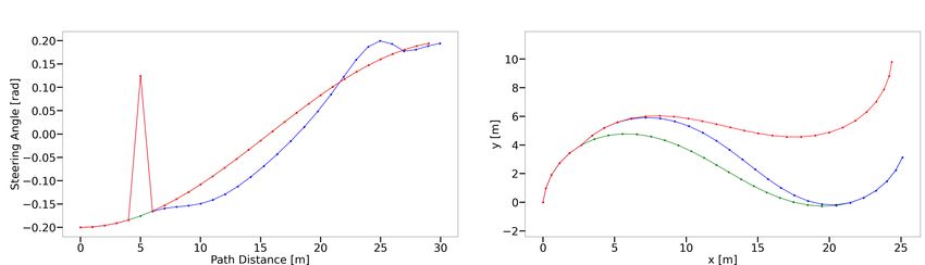
Fig. 5. Path perturbations in actuator space (left) and world space (right).
Green is the unperturbed path, red is perturbed with no correction, and blue
is perturbed with correction.
point’s steering angle (equation 14). Here vmin and vmax are
the minimum and maximum speeds, γ is the steering angle
at which we want the minimum speed, and pv , pφ are the Fig. 7. The test site used for the first experiment at the Texas A&M
steering angle and speed for the point p. Additionally, the RELLIS campus with a large rock pile covered in vegetation.
goal point is assigned a speed of zero.
B. Experimental Results
|pφ |
pv = vmin + (vmax − vmin )(1 − min( , 1)) (14) The following experiments were done at the Texas A&M
γ
RELLIS campus. This first test was done around a large rock
Next, backwards and forwards passes are done over the pile (figure 7). Figure 8 shows the test on the map. The goal
path such that all the path speeds lie within the maximum point was given on the other side of the pile. The line in red
and minimum acceleration limits of the vehicle. shows the initial A* path, the blue line shows the resulting
After this speed control pass the path is converted back optimized path. Note that the resulting path is similar to the
into world space and then published to the vehicle controller. input path but avoids the sharp turns in the base path. The
right figure shows the final driven path in yellow. We can
IV. RESULTS see that the driven path is initially similar to the first plan.
However, once the vehicle can see the other side of the rocks
A. System Overview the path is re-planned.
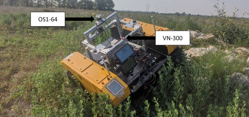
We tested this system on a Clearpath robotics Warthog.
The system architecture is described in figure 6. We equipped
it with an Ouster OS1-64 lidar and a Vectornav VN-300 INS.
Data from the IMU and wheel odometry was fused using an
extended kallman filter to provide fused odometry data. Our
map had a resolution of 20 cm with a size of 512x512 and
updated at a rate of 2 Hz. The A* planner was ran at 4 Hz
with the optimization module running at 10 Hz. The tests
were done with a speed of 5 m/s, the vehicle’s maximum
speed, and a minimum turning speed of 2 m/s.
Fig. 8. Driving around the rock pile with the initial plan (left) and final
path (right). Gray is free space, green is rough ground, bright orange is hard
obstacles, and dark orange is soft obstacles. The red path is the input path
to the optimizer, blue is the optimized path, and yellow is the driven path.
The goal point is represented by the pink circle.
In test 2 we go around a large hill (figure 9). Note that
the optimized path is significantly different from the base
path (figure 10). Unlike the first experiment, the terrain
around the hill is largely empty. Here, the planned path
didn’t significantly change as the robot moved, but controller
errors led to an overshoot of the first turn. However, this was
smoothly corrected and the resulting path was still collision
free.
C. Simulated Results
Fig. 6. A system overview of our test setup. The shaded region represents In addition to the real testing we also did several runs
the topic of this paper as represented in figure 2. in simulation. The simulator was created in the Unity game
engine and is integrated with the Robot Operating System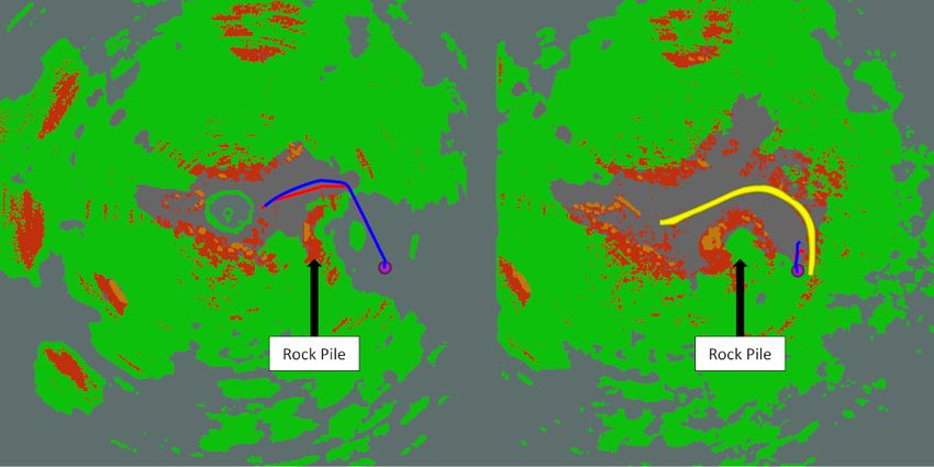
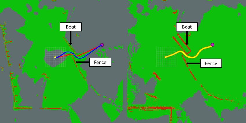
Fig. 12. A* sim results with the initial plan (left) and driven path (right).
Fig. 9. The test site used for the second experiment at the Texas A&M             The colors on the map represent different terrain features. Gray is unknown
RELLIS campus driving around a large hill.                                        space, green is ground, and dark orange is obstacles. The red path is the
                                                                                  initial a* path and yellow is the driven path. The goal point is represented
                                                                                  by the pink circle.

Fig. 10. Driving around a large hill with the initial plan (left) and final
path (right). The colors on the map represent different terrain features. Gray
is free space, green is rough ground, bright orange is hard obstacles, and        Fig. 13. Optimized results with the initial plan (left) and driven path (right).
dark orange is soft obstacles. The red path is the input path to the optimizer,   The colors on the map represent different terrain features. Gray is unknown
blue is the optimized path, and yellow is the driven path. The goal point is      space, green is ground, and dark orange is obstacles. The red path is the
represented by the pink circle.                                                   initial a* path, blue is the optimized path, and yellow is the driven path.
                                                                                  The goal point is represented by the pink circle.

(ROS). The simulation vehicle is a replica of the Warthog
used for the physical testing. Figure 11 shows the simulated                                                V. CONCLUSION
test environment. First we ran the system with the A* planner
as a baseline (figure 12). Next, the same path was ran with
                                                                                     We have developed a path optimization method for ground
our optimizer running on top of the A* path (figure 13). All
                                                                                  vehicles that is able to easily enforce kinematic constraints
other settings were left unchanged. A maximum speed of
                                                                                  onto the path. Using a gridded A* path as a base, this planner
5 m/s and a minimum speed of 2 m/s were used. The goal
                                                                                  was successfully able to operate at high speeds over off-road
point was set so the vehicle would go the small gap between
                                                                                  terrains.
the fence and boat. With only the A* path the vehicle would
overshoot the path and get stuck in the gap. Adding the                              Going forward we would like to extend this path opti-
optimizer allowed the vehicle to successfully navigate the                        mization method to speed control and temporal cost maps.
obstacles.                                                                        However, increasing the dimensonality of the problem would
                                                                                  also necessitate a more robust and efficient solver. By refin-
                                                                                  ing the cost function better properties could be expected.
                                                                                  These properties could then be exploited to more efficiently
                                                                                  solve the optimization function. Although, as terrain classi-
                                                                                  fication gets more complicated more layers to the costmap
                                                                                  will become necessary. This may increase the potential of
                                                                                  local minima and will be an important consideration in
                                                                                  future work. Additionally, planning in the actuator space
                                                                                  presents many opportunities for a tighter coupling between
                                                                                  planning and control. Finally, a mention should be made
                                                                                  about planning rate with increasing speed. To maintain a
                                                                                  constant reaction distance the total system latency must be
Fig. 11. The simulation environment showing the final position of the             inversely proportional to speed. Although planning is a large
Warthog after the A* baseline test.
                                                                                  part of the latency, to be successful at high speed operation
                                                                                  the entire system must be considered.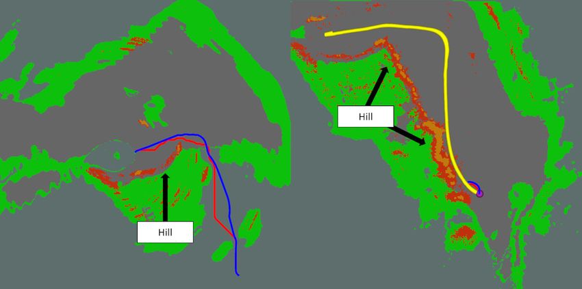
R EFERENCES                                              http://creativecommons.org/licenses/by/4.0/ (the “License”). Notwith-
                                                                                     standing the ProQuest Terms and Conditions, you may use this content
 [1] J. Luo and K. Hauser, “An empirical study of optimal motion
                                                                                     in accordance with the terms of the License; Last updated - 2018-11-
     planning,” in 2014 IEEE/RSJ International Conference on Intelligent
                                                                                     28; SubjectsTermNotLitGenreText - Japan.
     Robots and Systems, 2014, pp. 1761–1768.
                                                                              [12]   L. E. Dubins, “On curves of minimal length with a constraint on
 [2] Zhixin Chen, Mengxiang Lin, Shangzhe Li, and Rui Liu, “Evaluation
                                                                                     average curvature, and with prescribed initial and terminal positions
     on path planning with a view towards application,” in 2017 3rd Inter-
                                                                                     and tangents,” American Journal of Mathematics, vol. 79, no. 3,
     national Conference on Control, Automation and Robotics (ICCAR),
                                                                                     pp. 497–516, 1957. [Online]. Available: http://www.jstor.org/stable/
     2017, pp. 27–30.
                                                                                     2372560
 [3] N. Ratliff, M. Zucker, J. A. Bagnell, and S. Srinivasa, “Chomp:
                                                                              [13]   P. E. Hart, N. J. Nilsson, and B. Raphael, “A formal basis for the
     Gradient optimization techniques for efficient motion planning,” in
                                                                                     heuristic determination of minimum cost paths,” IEEE Transactions
     2009 IEEE International Conference on Robotics and Automation,
                                                                                     on Systems Science and Cybernetics, vol. 4, no. 2, pp. 100–107, 1968.
     2009, pp. 489–494.
                                                                              [14]   M. McNaughton, C. Urmson, J. M. Dolan, and J. Lee, “Motion
 [4] F. Z. Baghli, L. E. bakkali, and Y. Lakhal, “Optimization of arm
                                                                                     planning for autonomous driving with a conformal spatiotemporal
     manipulator trajectory planning in the presence of obstacles by
                                                                                     lattice,” in 2011 IEEE International Conference on Robotics and
     ant colony algorithm,” Procedia Engineering, vol. 181, pp. 560
                                                                                     Automation, 2011, pp. 4889–4895.
     – 567, 2017, 10th International Conference Interdisciplinarity in
                                                                              [15]   A. Stentz, “Optimal and efficient path planning for unknown and
     Engineering, INTER-ENG 2016, 6-7 October 2016, Tirgu Mures,
                                                                                     dynamic environments,” INTERNATIONAL JOURNAL OF ROBOTICS
     Romania. [Online]. Available: http://www.sciencedirect.com/science/
                                                                                     AND AUTOMATION, vol. 10, pp. 89–100, 1993.
     article/pii/S1877705817310184
                                                                              [16]   S. Koenig and et al., “Fast replanning for navigation in unknown
 [5] M. B. Horowitz and J. W. Burdick, “Combined grasp and manipu-
                                                                                     terrain,” 2002.
     lation planning as a trajectory optimization problem,” in 2012 IEEE
                                                                              [17]   S. LaValle, “Rapidly-exploring random trees : a new tool for path
     International Conference on Robotics and Automation, 2012, pp. 584–
                                                                                     planning,” The annual research report, 1998.
     591.
                                                                              [18]   G. M. van der Molen, Trajectory generation for mobile robots with
 [6] C. Richter, A. Bry, and N. Roy, Polynomial Trajectory Planning for
                                                                                     clothoids. Dordrecht: Springer Netherlands, 1992, pp. 399–406.
     Aggressive Quadrotor Flight in Dense Indoor Environments. Cham:
                                                                                     [Online]. Available: https://doi.org/10.1007/978-94-011-2526-0 46
     Springer International Publishing, 2016, pp. 649–666. [Online].          [19]   J. Choi and K. Huhtala, “Constrained global path optimization for
     Available: https://doi.org/10.1007/978-3-319-28872-7 37                         articulated steering vehicles,” IEEE Transactions on Vehicular Tech-
 [7] G. Kulathunga, D. Devitt, R. Fedorenko, S. Savin, and A. Klimchik,              nology, vol. 65, no. 4, pp. 1868–1879, 2016.
     “Path planning followed by kinodynamic smoothing for multirotor          [20]   M. Elhoseny, A. Tharwat, and A. E. Hassanien, “Bezier curve based
     aerial vehicles (mavs),” 08 2020.                                               path planning in a dynamic field using modified genetic algorithm,”
 [8] H. Oleynikova, M. Burri, Z. Taylor, J. Nieto, R. Siegwart, and                  Journal of Computational Science, vol. 25, pp. 339 – 350, 2018.
     E. Galceran, “Continuous-time trajectory optimization for online uav            [Online]. Available: http://www.sciencedirect.com/science/article/pii/
     replanning,” in 2016 IEEE/RSJ International Conference on Intelligent           S1877750317308906
     Robots and Systems (IROS), 2016, pp. 5332–5339.                          [21]   T. Maekawa, T. Noda, S. Tamura, T. Ozaki, and K. ichiro Machida,
 [9] W. Dong, Y. Ding, J. Huang, L. Yang, and X. Zhu, “An optimal                    “Curvature continuous path generation for autonomous vehicle using
     curvature smoothing method and the associated real-time interpolation           b-spline curves,” Computer-Aided Design, vol. 42, no. 4, pp. 350 –
     for the trajectory generation of flying robots,” Robotics and                   359, 2010. [Online]. Available: http://www.sciencedirect.com/science/
     Autonomous Systems, vol. 115, pp. 73 – 82, 2019. [Online]. Available:           article/pii/S0010448510000084
     http://www.sciencedirect.com/science/article/pii/S0921889017301173       [22]   K. Yang, D. Jung, and S. Sukkarieh, “Continuous curvature
[10] B. Li and Z. Shao, “Simultaneous dynamic optimization: A trajectory             path-smoothing algorithm using cubic b zier spiral curves for
     planning method for nonholonomic car-like robots,” Advances in                  non-holonomic robots,” Advanced Robotics, vol. 27, no. 4, pp. 247–
     Engineering Software, vol. 87, pp. 30 – 42, 2015. [Online]. Available:          258, 2013. [Online]. Available: https://doi.org/10.1080/01691864.
     http://www.sciencedirect.com/science/article/pii/S0965997815000708              2013.755246
[11] A. Ravankar, A. A. Ravankar, Y. Kobayashi, Y. Hoshino, and               [23]   T. Overbye and S. Saripalli, “Fast local planning and mapping in
     P. Chao-Chung, “Path smoothing techniques in robot navigation:                  unknown off-road terrain,” in 2020 IEEE International Conference
     State-of-the-art, current and future challenges,” Sensors, vol. 18,             on Robotics and Automation (ICRA), 2020, pp. 5912–5918.
     no. 9, 09 2018, copyright - © 2018. This work is licensed under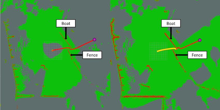
You can also read