QUALITY ANALYSIS OF FLOW FIELD DATA DETERMINED BY 3D PTV IN GAS FLOWS
←
→
Page content transcription
If your browser does not render page correctly, please read the page content below
12TH INTERNATIONAL SYMPOSIUM ON FLOW VISUALIZATION
                   September 10-14, 2006, German Aerospace Center (DLR), Göttingen, Germany

            QUALITY ANALYSIS OF FLOW FIELD DATA
             DETERMINED BY 3D PTV IN GAS FLOWS
                                      Torsten Putze
  TU Dresden, Insitiute for Photogrammetry and Remote Sensing, Helmholtzstraße 10, 0162
                                    Dresden, Germany

      Keywords: 3D-PTV, multi image analysis, spatio temporal matching, photogrammetry

ABSTRACT
     3D Particle Tracking Velocimetry (3DPTV) is a fully 3D flow measurement technique
delivering 3D velocity vectors and particle trajectories over large 3D observation volumes. The
paper shows the development of a 3D PTV system for application in gas flow, with observation
volumes ranging from (0.3 m)³ to (3 m)³. Adjusting the hardware components and the configuration
to the measurement task and using appropriate strategies, 3D point errors less than 1 mm can be
achieved in large observation volumes (up to some cubic metre). Results and achievable accuracies
are shown in two experiment configurations.

1 INTRODUCTION

3D Particle Tracking Velocimetry (3D PTV) is a flexible technique for the determination of 3D
velocity fields in liquid or gas. For that purpose a flow is densely visualised by particles and
recorded by a multi camera system. For each epoch 3D object coordinates are determined for all
tracer particles. Finally this method delivers time dependent 3D3C (3 dimensional, 3 component)
vector fields analysing the 3D trajectories of the seeded tracers. One measurement period consists of
either thousands of epochs or takes some seconds. The necessary hardware components to determine
the 3D object coordinates of each tracer particle are easy to handle and can be adapted to several
measurement tasks. Observation volumes up to some cubic metres can be realised. The analysis
algorithms are independent of size or velocity. Nevertheless, there is a limiting correlation between
the size of the observation volume, the size of the tracer particles, the image size, the frame rate of
the used camera and the necessary illumination. To determine a fast flow in a very large volume e.g.
a lot of hardware effort is necessary.

2 HARDWARE CONFIGURATIONS

In order to determine dynamic 3D object coordinates, at least two images taken synchronously are
necessary. In case of a densely seeded flow, four cameras are required to solve the ambiguities of
multi image matching [3] (cap 3.2). The used cameras are arranged convergent to achieve suitable
intersections. As mentioned before, there are correlations between observation volume, flow velocity
and camera characteristics. In [5] is shown, that a high speed camera system is essential to determine
high dynamic processes (cap.2.1). Considering the synchronisation and the costs of multi high speed
camera systems a mirror system is developed to generate virtual cameras and solve these problems
[6]. Large observation volumes require bigger image format. In case of some cubic metres

                                                                                                     1
Torsten Putze
observation volume SLR cameras (single lens reflex) are necessary to detect small tracer particles.
This leads to a very low frame rate so that only slow flows (chap 2.2) can be analysed.
2.1 Experiment A – drawn wind tunnel
For the development of new methods of 3D PTV several experiments are arranged in a draw tunnel
with a profile of 60 x 60 cm². Two boundaries are made of plexiglass as optical interface. Inside the
channel different objects are placed to analyse their influence on the flow field. The illuminated
observation volume covers 30 x 20 x 30 cm³ and the flow velocity is about 7 m/s. To determine the
drift of the used tracer particles additional free fall experiments in a low pressure tank are carried
out.
As mentioned before, a multi camera system is necessary to determine 3D object coordinates with
image based methods. In our case only one high speed camera with 1 MPixel image size is available.
By using a flexible four mirror system four virtual cameras with reduced active image size are
generated [7]. Figure 1 shows the image parts of the four virtual cameras on one sensor. The mirror
system can be modified to vary the intersection geometry and the observation volume. For the
mentioned experiments the mean distance between observation volume and cameras is 1 meter.
Besides the advantage of reduced hardware effort no synchronisation between the virtual cameras is
necessary. The disadvantage of this system is that one virtual camera consists of only one fourth of
the active image format. The slightly reduced accuracy caused by the mirror system is pointed out in
[6].
Fig. 1 – Mirror system on variable rails (left) and image parts of the four virtual cameras (right)
The used tracer particles for experiments in this draw channel are small Styrofoam spheres with
diameters of 0.1 or 0.5 mm. Although they do not have perfect flow following capability they are
easy to handle and to analyse. An approach to adjust the 3D trajectories affected by the tracer
characteristics is shown in [1]. The observation volume is illuminated by the fuzzy focal points of
halogen spot lights with fresnell lenses [5].
2QUALITY ANALYSIS OF FLOW FIELD DATA DETERMINED BY 3D PTV IN GAS FLOWS
2.2 Experiment B – ILKA
Another application for the developed algorithms of 3D PTV is the large scale convection in huge
cells (ILKA and Ilmenauer Fass) [8]. The cell ILKA is 3 x 3 x 4 m³ with the cameras and
illumination inside. Caused by the dimension of the observation volume four SRL cameras with an
image resolution of 8 MPixel are mounted in four corners of one boundary. This affords to detect the
tracer – in this case helium filled soap bubbles [2][8] – with diameters of less than 1 cm. Currently
halogen spot lights are used for the illumination. Because of the thermic sensibility of the cell other
illumination techniques have to be installed to avoid thermic input.
Due to the large depth range the tracer particles occur very densely in the images. Hence to solve the
multi image matching a high accuracy is necessary although the application’s main focus is turned to
large trajectories which represent the convection structures.
3 ANALYSIS CHAIN
The following chapter introduces the workflow of 3-D PTV. The flow chart shown in figure 2, points
out necessary steps of the workflow that is utilised in order to get 3D trajectories. The workflow can
be divided into three main parts: image processing, determination of object coordinates (spatial
matching) and tracking (temporal matching). The system calibration contains the determination of
the orientation and the characteristics of the cameras in a prior step. The single worl steps are
independent on each other. The observation volume and the velocity do not influence the analysis.
Image acquisition
Image pre-processing
Image analysis
System calibration
Multi image matching
Object coordinates
Tracking 2D / 3D
3D trajectories
Fig. 2 – Workflow
3Torsten Putze
3.1 Image processing
In order to extract image coordinates with sub-pixel precision, the following steps are applied to the
image sequences: First a background image is created by a temporal histogram analysis. This is
subtracted from all original images. In the created difference images, discrete tracer particles are
segmented by a region growing approach supported using a discontinuous criterion [4]. This has to
be done to divide overlapping tracer particles. Applying a centroid algorithm, the image coordinates
are determined with sub-pixel precision. The centroid of an object blurred by velocity is close to the
average position during the exposure time [10]. Consequently, the blurring does not influence the
image coordinates significantly (in case of linear movement). Furthermore the blurring includes
information about the motion direction of each tracer particle. This can be used as additional
knowledge for the temporal matching.
3.2 Object coordinate determination
The 3D object coordinates are calculated from the image coordinates of homologous image points.
Therefore, it is necessary to link all related image points representing one tracer in the object space.
This matching is supported using the epipolar constraint and approximate depth information about
the point cloud. In case of using only two images, all image points within a certain distance to the
epipolar line are candidates, thus ambiguities cannot be solved in a densely packed flow. A third
camera reduces the search space for corresponding particles from a line (plus tolerance) to the
intersection points of lines (Figure 3)[3]. It can be shown that the use of a third camera reduces the
probability of occurrence of ambiguities by the factor 10...100. For most applications an
unambiguous solution is possible. This requires that the orientation parameters are well determined
and every tracer particle is represented in each image. If this is not the case, ambiguities cannot be
solved or tracer positions get lost.
Fig. 3 – Solving multi image matching using epipolar lines in 3 images (following [4])
90% of the remaining ambiguities can be solved using a fourth camera. This provides much more
information. Hence, weaker camera orientations or hidden particles in an image can also be
successfully analysed. Because of the higher amount of information, other ambiguities have to be
solved. Using image point triples, the image point in the fourth image can be calculated. If there is
no candidate in the search area, there are two possibilities: The tracer can be hidden or the candidates
of the image point triple are no homologous image points. Whether the object point is calculated
with three of four image points or not, is decided by a probability based algorithm.
4QUALITY ANALYSIS OF FLOW FIELD DATA DETERMINED BY 3D PTV IN GAS FLOWS
3.3 Spatial matching
After image processing to determine the object coordinates of all epochs, lots of unconnected point
clouds are available. At that time they do not include any information about the velocity field. There
are different approaches to calculate this information. They can be global or local in two or three
dimensional data sets [9]. The used tracking algorithm is local and spatial based. This means that for
each object coordinate triple (each tracer and each epoch) a position in the following epoch is
predict. Using decision rules and connectivity analysis long trajectories with 5 to 80 nodes
(maximum depends on the residence time in the observation area) can be generated.
Using the tracking in image space additionally the redundancies of multi image matching and
tracking can be used for a loop check. As shown in [1] it will be necessary to correct the tracer path
because of their drift. This means that the original trajectories do not represent the flow field but for
each node a corrected velocity vector can be determined.
4 RESULTS
As one can see in the analysis chain different results are available. There are object coordinates of all
tracers at all epochs. All of these unique coordinate triples belong to the same accuracy level and are
not correlated (except the orientation parameters). The accuracy potential depends on the image
point measurement, the system orientation and the object size respectively the distance between
camera and target.
These independent 3D positions lead to positive effects of the trajectory accuracy. One trajectory
consists of two nodes. It is obvious that the length of the vector (distance between two nodes)
influences its accuracy concerning the length and the direction. Figure 4 shows this effect and reason
that long single trajectories (distance between two nodes) consist of a higher relative accuracy. Long
connected trajectories (lots of nodes) can be smoothed to improve the single node accuracy.
Target position
with point error
Actual position
t1 t2 t3 t1 t2 t3
Fig. 4 – Influence of point error on length and direction of trajectories
The used tracking algorithm has to consider the ration between 3D object coordinate accuracy and
trajectory length. A correct prediction to the succeeding epoch depends on the true direction (in case
of long trajectories) or the true length (in case of short trajectories). Using error propagation
(equation (1)) of 3D point error (σPt1/σPt2) it is possible to determine the error of the prediction for
the spatial matching and to adapt the matching parameters.
2 2 2
∂P ∂P ∂P
= t 3 ⋅ σ l + t 3 ⋅ σ r + t 3 ⋅ σ Pt 2
2
σP (1)
t3
∂l ∂r ∂Pt 2
5Torsten Putze
2 2
∂l ∂l
= ⋅ σ Pt1 + ⋅ σ Pt 2
2
σl (2)
∂Pt1 ∂Pt 2
2 2
∂r ∂r
= ⋅ σ Pt 1 + ⋅ σ Pt 2
2
σr (3)
∂Pt1 ∂Pt 2
The absolute accuracy does not depend on the size of the observation volume, the flow velocity or
the used frame rate. In contrast the relative accuracy is higher with growing flow velocity and longer
trajectories. But it is obvious that in this case the pre processing is more difficult [5].
4.1 Object coordinates
There are two different experiments called A (draw wind tunnel) and B (ILKA cell). Their
configuration parameters are shown in table 1.
Characteristic Experiment A1 / A2 (draw channel) Experiment B (ILKA cell)
Size 40 x 40 x 40 cm³ 4 x 3 x 4 m³
Tracer particles Styrophoam 0.1 – 0.5 mm Helium filled soap bubbles 1 cm
Camera system High-speed camera-mirror system 4 SRL cameras
Pixel number and size 1 MPx - 12µm 8 MPx - 6.42 µm
Mean distance camera - tracer 1.5 m / 0.9 m 3m
Mean base length 0.45 m 2.10 m
Base-depth ratio 1 : 3.3 / 1 : 2 1 : 1.4
Tab. 1 – Parameters of the experiments
The results can be evaluated using the standard deviations of each calculation step. At first the
calibration target field with dot and code marks is determined with high accuracy. The standard
deviations of these 3D points are shown in table 2.
Experiment A Experiment B
Size 30 x 50 x 5 cm³ - calibration board 3 x 3 x 1 m³ - cell boundary
Point number 289 91
Standard deviation – lateral 3 µm 0.10 mm
Standard deviation – depth 6 µm 0.15 mm
Tab. 2 – Properties of calibration fields
The orientation parameters of all cameras are determined within a resection. The resulting standard
deviation of unit weight represents the accuracy potential of the used configuration (table 3). To
demonstrate the potential, standard deviations are translated to point errors in the mean observation
volume. Tapping the full potential requires same conditions as at the calibration. The image point
measurement accuracy of 1/50 Pixel (Px) for dot marks using ellipsoid operator can not be achieved.
Caused by shape and size of the tracer particles the centroid algorithm with a less sub-pixel accuracy
6QUALITY ANALYSIS OF FLOW FIELD DATA DETERMINED BY 3D PTV IN GAS FLOWS
is necessary. Furthermore, using a mirror system in experiment A reduces the accuracy potential by
factor 2-3 [6].
Experiment A1 Experiment A2 Experiment B
σ0 1.4 µm ≈ 1/9 Px 1.4 µm ≈ 1/9 Px 0.4 µm ≈ 1/15 Px
Lateral point error in mean distance 0.08 mm 0.05 mm 0.09 mm
Depth point error in mean distance 0.28 mm 0.10 mm 0.12 mm
Tab. 3 – Accuracy potential
The analysis of experiments using intersection yields 3D object coordinates with related standard
deviations (table 4). Processing thousands of epochs with hundreds of tracers the determined
accuracies show reliable values for the used measurement system. Different orders of magnitude in
accuracy are caused by the different configurations and used cameras.
Experiment A1 Experiment A2 Experiment B
σX 0.15 mm 0.07 mm 0.6 mm
σY 0.15 mm 0.06 mm 0.6 mm
σZ 0.50 mm 0.12 mm 1.0 mm
Tab. 4 – Standard deviation of 3D object coordinates of tracer particles
Using more hardware effort in experiment A – especially more cameras with higher resolution – the
accuracy will be enhanced by factor 3. Aim of experiment B is to analyse large scale structures.
There it is not to achieve high single point accuracy but determine large connected trajectories. The
resulting trajectories depending on the one hand on the 3D point accuracy but also on the length of
vectors and trajectories.
4.2 Trajectories
Basic elements of a trajectory are vectors of one tracer in successive epochs. Quality criteria are
cumulative length over all epochs and accuracy of each partial vector. The length and direction error
of vectors caused by 3D point error of the nodes can be calculated with equations (2) and (3). The
maximum number of a trajectory is limited by the residence time in the observation volume. It is also
constrict by the number of epochs taken with the measurement system. Mostly the memory writing
rate of cameras is the limiting fact.
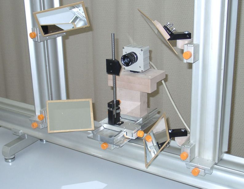
Figure 5 shows some representative trajectories of both experiments A and B. One example of
experiment A consists of 1000 epochs within 2 seconds. The longest trajectory contains 61 vectors.
All trajectories in figure 5 left are longer than 20 epochs. The mean vector length averages 12 mm.
Table 5 gives an overview about the length of the 3787 determined trajectories.
# vectors ≥ 30 ≥ 25 ≥ 20 ≥ 15 ≥ 10 10 to 4
# trajectories 5 4 75 749 1022 1932
Tab. 5 – Number and length of trajectories
7Torsten Putze
Fig. 5 – Trajectories behind a cylinder (left – experiment A), trajectories over a ventilator (right – experiment B)
An example of experiment B contains 20 epochs caused by the storage capacity of the used SLR
cameras. Table 6 shows the distribution of the trajectory lengths. The mean vector length averages
30 mm. The system was triggered manual so velocities can not be calculated.
# vectors ≥ 15 ≥ 10 ≥ 5
# trajectories 6 5 36
Tab. 6 – Number and length of trajectories
4.3 Further analysis
The determined trajectories describe the path of each particle. Caused by the properties of the tracer,
each velocity vector within a trajectory has to be corrected as shown in [1]. This leads to a not
connected trajectory but gives at a current position and time a 3C velocity vector. For further
analysis an interpolation to a regular grid can be processed.
To verify the system some experiments with defined motions and comparable experiments to
established flow measurement systems will be carried out.
5 CONCLUTION
In this article we present the 3D Particle Tracking Velocimetry (3D PTV) measurement system and
its potential for flow field determination. It affords to determine a time resolved 3D3C flow field
while either hundreds of epochs or some seconds. Modifying the hardware configuration several
large observation volumes (up to some cubic metres) can be analysed.
The accuracy depends on a lot of parameters. It is shown that a 3D point error of less than 1/10 mm
in smaller and 1 mm in large volumes can be achieved. The accuracy of trajectories depends on their
lengths and on 3D point errors of their nodes.
8QUALITY ANALYSIS OF FLOW FIELD DATA DETERMINED BY 3D PTV IN GAS FLOWS
6 ACKNOLEDGEMENT
The work presented in this paper was supported by “Deutsche Forschungsgesellschaft” (DFG) within
the SPP 1147. The author’s gratitude also goes to Dr. K. Hoyer (IHW, ETH Zurich) for producing
hardware components of the mirror system and to the “Institut für Luft- und Raumfahrttechnik” for
supporting my experiments.
REFERENCES
1. Frey J, Putze T and Grundmann R. Räumliches PTV in Gasströmungen und Ansätze zur Korrektur des
begrenzten Partikelfolgevermögens. Proceedings der 14. GALA-Fachtagung "Lasermethoden in der
Strömungsmeßtechnik”, Braunschweig, 2006.
2. Machacek M and Rösgen T. A Quantitative Visualization Method for Wind Tunnel Experiments Based
on 3D Particle Tracking Velocimetry (3D-PTV). PAMM, Proc. Appl. Math. Mech. 1, 2002.
3. Maas H-G. Complexity analysis for the determination of image correspondences in dense spatial target
fields. International Archives of Photogrammetry and Remote Sensing, Vol. 29, Part B5, pp 102-107,
1992.
4. Maas H-G, Grün A and Papantoniou D. Particle tracking in threedimensional turbulent flows. Part I:
Photogrammetric determination of particle coordinates. Experiments in Fluids, Vol. 15, pp 133-146, 1993.
5. Putze T. Einsatz einer Highspeedkamera zur Bestimmung von Geschwindigkeitsfeldern in Gas-
strömungen. 24. wissenschaftlich- technische Jahrestagung der DGPF, pp 325 – 332, 2004.
6. Putze T. Geometric modelling and calibration of a virtual four-headed high speed camera-mirror system
for 3-D motion analysis applications. Optical 3-D measurement techniques VII, pp 167 – 174, 2005.
7. Putze T and Hoyer K. Modellierung und Kalibrierung eines virtuellen Vier-Kamerasystems auf Basis
eines verstellbaren Spiegelsystems. Beiträge der Oldenburger 3D-Tage 2005, Herbert Wichmann Verlag,
Heidelberg, 2005.
8. Resagk C, Lobutova E, Rank R, Müller D, Putze T and Maas H-G. Measurement of large-scale flow
structures in air using a novel 3D Particle Tracking Velocimetry technique. 13th Int. Symp on Appl. Laser
Techniques to Fluid Mechanics, Lisbon, Portugal, 2006.
9. Ruhnau P, Gütter C, Putze T, Nobach H and Schnörr C. A Variational Approach for Particle Tracking
Velocimetry. Measurement, Science & Technology 16, pp 1449 – 1458, 2005.
10. Wierzimok D and Hering F. Quantitative Imaging of Transport in Fluids with Digital Image Processing.
Imaging in Transport Processes, Begell House, pp 297-308, 1993.
9You can also read