Radar-Inertial Ego-Velocity Estimation for Visually Degraded Environments
←
→
Page content transcription
If your browser does not render page correctly, please read the page content below
Radar-Inertial Ego-Velocity Estimation for Visually Degraded
                                 Environments
                                  Andrew Kramer, Carl Stahoviak, Angel Santamaria-Navarro,
                                    Ali-akbar Agha-mohammadi and Christoffer Heckman

   Abstract— We present an approach for estimating the body-                                LORD 3DM-GX5-15 IMU (not shown)   Hokuyo URG 2D LiDAR
frame velocity of a mobile robot. We combine measurements                                                                     (not used in this work)

from a millimeter-wave radar-on-a-chip sensor and an inertial                        Intel T265 Tracking Camera

measurement unit (IMU) in a batch optimization over a sliding
window of recent measurements. The sensor suite employed
is lightweight, low-power, and is invariant to ambient lighting
conditions. This makes the proposed approach an attractive
solution for platforms with limitations around payload and
longevity, such as aerial vehicles conducting autonomous explo-
ration in perceptually degraded operating conditions, including
subterranean environments. We compare our radar-inertial
velocity estimates to those from a visual-inertial (VI) approach.
                                                                                     TI AWR1843BOOST Radar SoC                         Intel NUC7-i7
We show the accuracy of our method is comparable to VI in
conditions favorable to VI, and far exceeds the accuracy of VI
when conditions deteriorate.
                                                                            Fig. 1. Experimental sensor rig consisting of 77–81 GHz FMCW radar,
                        I. I NTRODUCTION                                    Intel RealSense T265 tracking camera, LORD microstrain IMU and Intel
                                                                            NUC onboard computer.
   Accurate and reliable estimates of ego-velocity are crucial
for closed-loop control of autonomous mobile robots during
                                                                            is a popular option for robots operating in darkness, smoke
navigation operations. This is especially true for fast-moving
                                                                            or fog [2], but these methods track temperature gradients,
robots like micro aerial vehicles (MAVs). Robot body-frame
                                                                            which are often not present in subterranean environments.
velocities are commonly estimated using some combination
                                                                            Thus, it is clear that there exists a need for a reliable and
of visual, LiDAR, inertial and/or GPS sensors. Accurate ego-
                                                                            efficient method for ego-velocity estimation which is capable
velocity estimates are intrinsic to any number of simultane-
                                                                            of generalizing across diverse environments and operating
ous localization and mapping (SLAM) methods that have
                                                                            conditions.
been developed. For those methods that rely on visual data,
                                                                               Millimeter wave radar is an attractive option for subter-
the quality of the ego-velocity estimate is quickly degraded
                                                                            ranean environments. It does not require light or temperature
in darkness, feature-poor environments, and so forth. Here,
                                                                            gradients to operate. Additionally, automotive-grade system-
we consider the subterranean environment as a motivating
                                                                            on-chip (SoC) radars have low power requirements. How-
example.
                                                                            ever, radar measurements are adversely affected by sensor
   Robust autonomy in subterranean environments is cur-
                                                                            noise and radar-specific corruptions of data, e.g. multipath
rently a popular research topic. NASA is planning to explore
                                                                            reflections and binning of spatial and Doppler measurements.
caverns on the moon and Mars [1], while DARPA is conduct-
                                                                            So, while it is certainly possible to estimate a robot’s body-
ing its Subterreanen Challenge1 . Most state-of-the-art meth-
                                                                            frame velocity from standalone radar data using robust
ods for body-frame velocity estimation are significantly im-
                                                                            optimization techniques [3], these estimates are not suffi-
paired in conditions common to subterranean environments,
                                                                            ciently accurate for reliable control. Additionally, the antenna
e.g. GPS data is unavailable and cameras cannot capture
                                                                            pattern of the radar will naturally provide more accuracy
useful information in complete darkness. Thermal imaging
                                                                            in some dimensions than others. In order to overcome the
    A. Kramer, C. Stahoviak and C. Heckman are with the De-                 shortcomings of radar as a standalone sensor, it is beneficial
partment of Computer Science at University of Colorado, Boulder,            to fuse radar and inertial measurements.
Colorado 80309, USA {andrew.kramer; carl.stahoviak;                            This work presents a method for ego-velocity estimation
christoffer.heckman}@colorado.edu
    A. Santamaria-Navarro and A. Agha-mohammadi are with the Jet            that uses an automotive-grade radar SoC (Texas Instruments
Propulsion Laboratory, California Institute of Technology, 4800 Oak Grove   AWR1843) and a MEMS IMU. We use Doppler velocity
Dr, Pasadena, CA 91109, USA {angel.santamaria.navarro;                      measurements to estimate the body-frame velocity of the
aliakbar.aghamohammadi}@nasa.jpl.gov
    This work was supported through the DARPA Subterranean Challenge,       sensor at the time of each radar measurement. We jointly esti-
cooperative agreement number HR0011-18-2-0043. Part of this research        mate ego-velocities over a sliding window of the previous K
was carried out at the Jet Propulsion Laboratory, California Institute of   radar measurements in a nonlinear optimization framework,
Technology, under a contract with the National Aeronautics and Space
Administration.                                                             using IMU measurements to constrain the change in velocity
  1 https://www.subtchallenge.com                                           between radar measurements. The addition of inertial data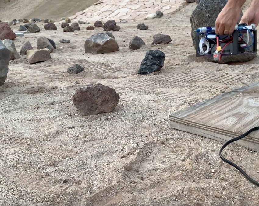
Fig. 3. Factor graph representation of the radar-inertial velocity estimation
system. States from N previous timesteps are jointly estimated using
Doppler targets and sets of IMU measurements as constraints
estimate ego-velocity, they are ill-equipped for use in envi-
ronments with challenging sensing conditions.
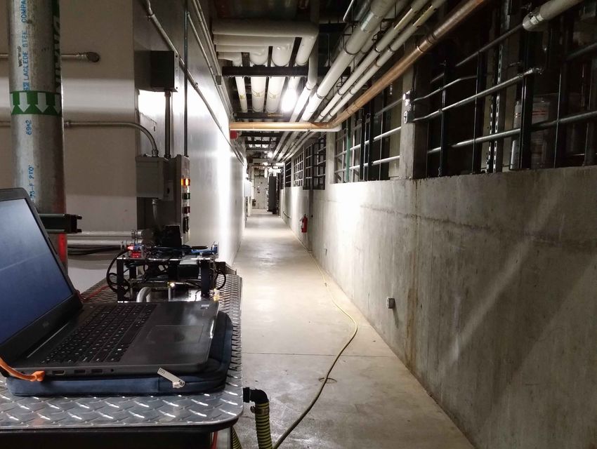
Fig. 2. Example of the subterranean analog environment in which we Like our method, several previous state estimation systems
tested: the steam tunnels beneath Folsom Field at CU Boulder. have been formulated as maximum a posteriori estimation
problems represented by factor graphs [17]. These include
helps to smooth the high noise that would be present if we the popular visual method ORB-SLAM [18], [19] and the
were estimating body-frame velocity from radar data alone. visual-inertial method OKVIS [20] from which our radar-
Conversely, velocity estimates from the radar are drift-free, inertial method draws considerable inspiration.
so the radar information allows us to estimate the biases of Our method represents a significant advance over previous
the IMU. methods in several important ways. First, our method is ap-
This paper is organized as follows. Section II reviews plicable to 3 dimensional environments, while the previously
related work in the area of ego-velocity estimation. Sec- mentioned radar state estimation methods are only applicable
tion III details our velocity estimation method. Section to 2D environments. This means that our method is usable
III-A briefly describes how Doppler velocity and inertial on micro aerial vehicles and other robots that do not operate
constraints are combined to accurately estimate the sensor in planar environments. Second, our method fuses radar and
platform’s body-frame velocity. Section III-B describes how inertial measurements, providing highly accurate estimates
body-frame velocity can be estimated from millimeter wave and constraining the large uncertainty normally associated
radar data and how the Doppler residual is formulated in our with radar-based methods. Previous radar state estimation
optimization. Section III-C explains the IMU kinematics used methods have used radar as their sole sensor and robotic
in our problem and how the inertial constraint is formulated. sensor fusion methods with radar have only been minimally
We then highlight the process for experimentally validating explored. Lastly, previous radar-based state estimation meth-
our method in Section IV. Finally, we discuss our results and ods have either depended on highly specialized scanning
conclusions in Sections V and VI, respectively. sensors [5], [6], [9] or arrays of several automotive sensors
requiring precise extrinsic calibration [7], [8]. Our method
II. RELATED WORK requires only one single-board radar sensor and an IMU, and
While radar is well-established in the automotive industry thus the sensor package we employ is simpler than those used
and has been used for various tasks in vehicle autonomy in previous methods.
including collision avoidance, automated braking, lane keep- III. M ETHODOLOGY
ing, autonomous parking, etc. [4], very few methodologies
for using radar as a primary sensor for ego-motion estimation A. System Structure
have been presented in the literature. The most consequen- Our approach estimates the body-frame velocity of the
tial of these have focused on odometry and SLAM using sensor platform over a sliding window [21] of K previous
only millimeter wave radar. [5] presents methods for radar radar measurements. These velocities are linked by integrated
landmark detection, scan matching, and odometry in diverse accelerometer measurements from the IMU. Figure 3 shows
and challenging conditions; this work is extended in [6]. a factor-graph representation of our system’s structure.
Additionally [7] and [8] have presented methods for radar- Accelerometer measurements are affected by both bias ba
based SLAM using arrays of automotive-grade radar sensors. and gravity gW . Velocity estimates from radar are bias free,
Lastly, [9] made use of Doppler velocity measurements for so we can compensate for the accelerometer biases by simply
body-frame velocity estimation as part of their odometry including them in the state vector. Compensating for gravity
system. is more complicated, however. To do this we need to estimate
Additionally, good results for ego-velocity estimation have the IMU’s attitude (pitch and roll), which we represent as the
been obtained using stereo camera configurations and RGB- orientation quaternion qW S . In order to estimate the IMU’s
D sensor systems [10], [11], [12]. The use of a smart camera attitude, we need to use gyro measurements and to do this we
(optical flow), an IMU and a range sensor is proposed in [13] must also estimate the gyro biases bg . The full state vector
and [14]. Similarly, methods like [15] take advantage of a is then given as x = [vST , qTW S , bTg , bTa ]T .
LiDAR or a combination of LiDAR and IMU measurements We formulate our radar-inertial ego-velocity estimation as
as in [16]. Although these approaches are able to efficiently an optimization over the cost function
and attitude. The states are propagated via the following
K X K−1
X X T differential equations:
J(x) := ed w d + eks Wsk eks (1)
k=1 d∈D k k=1
1
| {z } | {z }
Doppler term inertial term
q̇W S = Ω(ωS )qW S
2
where K is the number of past radar measurements for which v̇S = aS + CSW gW − (ωS ) × vS
states are estimated, Dk is the set of targets returned from (5)
the radar measurement at time k, ed is the Doppler velocity ḃg = wbg
error, es is the IMU error. The error terms are weighted by 1
ḃa = − ba + wba
the information matrix Ws in the case of the IMU errors; and τ
the normalized intensity of the corresponding radar target
The elements of w := [wgT , waT , wbTg , wbTa ]T are zero-
ij mean, uncorrelated Gaussian white noise, gW is the gravity
wdj = P (2)
d∈D id vector in the world frame, and CSW is the rotation matrix
specifying the rotation from the world frame of reference to
in the case of the Doppler velocity measurements where wdj the sensor frame. The gyro and accelerometer measurements,
is the weight for target j in scan D and ij is the intensity of ω̃S and ãS respectively, are defined as the true acceleration
target j. In the following sections we detail the formulation and angular rate with added bias and white noise
of our Doppler and IMU measurement constraints.
B. Estimating Ego-Velocity From Doppler Velocity Measure- ω̃S = ωS + bg + wbg
ments (6)
ãS = aS + ba + wba
A radar measurement consists of a set of targets D. Each
d ∈ D consists of [rS , vR , θS , φS ]T , the range, Doppler and the matrix Ω is formed from the estimated angular rate
(radial) velocity, azimuth, and elevation for target d. The as
Doppler velocity measurement vR is equal to the magnitude
of the projection of the relative velocity vector between the
−ωS
⊕
target and sensor vS onto the ray between sensor origin and Ω(ωS ) := (7)
1
the target rS . This is simply the dot product of the target’s
velocity in the sensor frame and the unit vector directed from The ⊕ operator is defined in [23].
the sensor to the target In order to optimize over this model we need the lin-
!T earized, discrete time version of the state equations in Eq.
rS (5). First, the continuous time state transition matrix is
vR = v S (3)
krS k
We assume the targets in the scene are stationary and only 03×3 03×3 C̄W S
03×3
the sensor platform is moving. In this case each radar target −C̄W S [gW ]× −[ωS ]× −[vS ]×
−I3×3
Fc (x) =
can provide a constraint on our estimate of the sensor rig’s 03×3 03×3 03×3
03×3
velocity in the body-frame. The velocity error for each radar 03×3 03×3 − τ1 I3×3
03×3
target is then (8)
where the [.]× operator denotes the skew symmetric matrix
!T
ri,k associated with the cross product of the vector. Next, an
i,k
k k
e (x , d i,k
)= vR − vSk S
(4) approximate discretization of Fc is found via Euler’s method
kri,k
S k
where xk is the state at time k and di,k is the ith target in the Fd (x, ∆t) = I + Fc (x)∆t (9)
set of radar measurements at time k. As previously noted,
radar measurements are affected by non-Gaussian noise and and the covariance is propagated as
radar scans often contain false target data. These challenges
are addressed by using the Cauchy robust norm with the
Doppler residual. Pk+1 =
(10)
Fd (x̂k , ∆t)Pk Fd (x̂k , ∆t)T + G(x̂k )QG(x̂k )T
C. Formulation of the IMU Constraint
1) IMU Kinematics: In our system, the IMU’s accelerom- where Q := diag(σg2 , σa2 , σb2g , σb2a ) and
eter readings are used to measure the system’s change in
body-frame velocity between radar measurements. Our IMU
C̄W S 03×3 03×3 03×3
model is very similar to those used in OKVIS [20] and 03×3 I3×3 03×3 03×3
G(x) = (11)
MSCKF [22], except we do not use the IMU to measure
03×3 03×3 I3×3 03×3
the change in the system’s full pose, only its velocity 03×3 03×3 03×3 I3×3Fig. 4. Different rates of IMU and radar sensor. One IMU term uses all
accelerometer and gyro readings between successive radar measurements.
Additionally, gyro and accelerometer readings at times 0 and R are
interpolated from the adjacent measurements.
2) IMU Error: The IMU provides measurements at many
times the rate of the radar sensor. Further complicating mat-
ters, the IMU and radar measurements are not synchronized. Fig. 5. Data collection in the Mars yard at the NASA Jet Propulsion
This is illustrated in Fig. 4. Laboratory.
Between radar measurements at timesteps k and k + 1
several IMU measurements occur. We interpolate between To estimate groundtruth body-frame velocity of the sensor
the IMU measurements immediately before and after the rig, we use measurements from a Vicon motion capture sys-
radar measurements to obtain estimated IMU readings that tem and an IMU onboard the vehicle platforms. The Vicon
align temporally with the radar measurements. The state system provides drift-free pose measurements. However, the
at k + 1, x̂k+1 , is estimated by iteratively applying the transform between the Vicon system’s coordinate frame and
propagation equations in Eq. (5) using the Euler forward the vehicle’s coordinate frame is unknown. Additionally, the
method. The IMU error is then defined as Vicon measurements are subject to both noise and communi-
cation latency between the Vicon system and the host system.
h
k+1 −1
i Thus, IMU measurements are used to estimate the transform
2 q̂k+1
W S ⊗ qW S between the Vicon coordinate frame and the vehicle’s body-
1:3
v̂Sk+1 − vSk+1 frame, the timestamp offsets between the Vicon system and
ek (xk , xk+1 , zk ) = (12)
host system, and to smooth noise in the Vicon measurements,
b̂g − bg
b̂a − ba similar to [24].
where the ⊗ operator is as defined in [23]. The Jacobian of B. Evaluation Procedure
the error with respect to the state at k + 1 is defined as To evaluate our method, we create a new dataset of radar
and inertial data using the sensors previously described. In
h i⊕ addition to radar and inertial data, we record Vicon data
k+1 −1
∂ek q̂ k+1
⊗ q 03×9 when available for groundtruth. Lastly, for comparison we
= W S W S
1:3,1:3 (13)
∂ χ̂k+1 0 I9×9 use the visual inertial odometry (VIO) output from an Intel
9×3
Realsense T265.
The Jacobian with respect to the state at time k is somewhat We conducted experiments using the handheld sensor rig
more difficult to calculate because the IMU error term is shown in Fig. 1. Several of these were done in the steam
found by iteratively applying the IMU integration. Differen- tunnels beneath Folsom Field at CU Boulder to simulate a
tiating the error with respect to the state at time k requires subterranean environment, and outdoors in the Mars yard at
use of the chain rule, leading to NASA’s Jet Propulsion Laboratory. These environments are
pictured in Fig. 2 and Fig. 5, respectively. These runs do
not include groundtruth data so the performance of the two
R
!
∂ek Y ∂ek
= i i
Fd (x̂ , ∆t ) (14) methods is compared qualitatively. Here we seek to demon-
∂ χ̂k ∂x̂k+1
i=0 strate that when VIO works our radar-inertial method’s
IV. E XPERIMENTS performance is comparable to VIO and when VIO fails our
method continues to work.
A. Sensor Setup The steam tunnel runs are between 60 and 120 seconds
To demonstrate our method we use an automotive grade in length and are conducted in bright and dark conditions.
radar-on-chip sensor, Texas Instruments AWR1853. The sen- The Mars yard runs were roughly 60 seconds in length.
sor operates in the 77-81 GHz band and identifies targets These were done with the sensor rig close to the ground,
within a field-of-view (FOV) of approximately ± 75 degrees as would be the case for a planetary rover. Also, the Mars
azimuth and ± 20 degrees elevation. The sensor produces a yard experiments were conducted near sunset. This created
maximum of 160 targets per measurement at a rate of 10 Hz. challenging lighting conditions for VIO with large brightness
For inertial sensing we employ a LORD Microstrain 3DM- gradients, shadows, and a very bright sky near the horizon
GX5-15 IMU. The extrinsic transform between the IMU and which would make it difficult to obtain properly exposed
radar coordinate frames was manually measured. images.TABLE I
C ONDITIONS IN WHICH EXPERIMENTS WERE RUN . E ACH LISTED 1.5
vx error (m/s)
EXPERIMENT WAS RUN THREE TIMES .
1
Location Motion Lighting Platform Groundtruth 0.5
CU Vicon Space Fast Bright Quadrotor Vicon
CU Vicon Space Slow Bright Quadrotor Vicon 0
0 5 10 15 20 25 30 35
CU Vicon Space Fast Dim Quadrotor Vicon
CU Vicon Space Fast Dark Quadrotor Vicon time (s)
CU Steam Tunnels Slow Bright Handheld None
CU Steam Tunnels Slow Dark Handheld None 1.5
vy error (m/s)
JPL Mars Yard Slow Bright Handheld None
1
TABLE II 0.5
M EAN AND STD DEVIATION OF RMS VELOCITY ERROR IN M / S FOR
QUADROTOR EXPERIMENTS (N = 3) 0
0 5 10 15 20 25 30 35
time (s)
Lighting bright bright dim dark
Movement slow fast fast fast 1.5
vz error (m/s)
µ σ µ σ µ σ µ σ
1
x .10 .025 .20 .021 .20 .030 .56 .012
VIO y .26 .012 .19 .014 .23 .021 .31 .018 0.5
z .17 .021 .31 .030 .31 .009 .40 .013
x .10 .011 .21 .006 .19 .016 .16 .013 0
RI y .16 .015 .28 .009 .25 .017 .17 .020 0 5 10 15 20 25 30 35
z .11 .025 .28 .006 .25 .024 .14 .017 time (s)
Fig. 6. Body-frame velocity estimate error from our method and VIO for
The same sensor suite was also mounted on a quadrotor an example run in ideal sensing conditions for VIO. Errors for VIO are
plotted in blue and ours are plotted in red.
for experiments in our motion capture space. These quadrotor
runs varied between 30 and 60 seconds in length, featured
both slow, smooth motions and fast, aggressive motions, and for multiple seconds then the IMU constraints will not be
were conducted in bright, dim, and dark conditions. Each of sufficient to smooth out the noise in the radar measurements.
these experiments was run 3 times in the same conditions This can be seen around the 10 second mark in the vy error
and over the same path. All of these runs have groundtruth plot of figure 6. This issue may be addressed in future work
from motion capture. For these runs, we are able to quantify by adding a term to the optimization that approximates the
the accuracy of VIO and our radar-inertial method in terms influence of measurements that have passed out of the sliding
of the root mean squared error (RMSE) between the ego- window.
velocity estimate and the groundtruth:
Figure 7 shows the estimated ego-velocity components
s
PN for an example run conducted in dark conditions in our
i i 2
i=1 (vest − vgt ) motion capture space. The velocity estimates from RI track
vRMSE = (15)
N the groundtruth closely, while the estimates from VIO often
The runs included in our dataset are summarized below in have large deviations. This demonstrates that the proposed
table I. method continues to function normally in dark conditions
while VIO’s performance suffers. Additionally, Fig. 8 shows
V. R ESULTS the ego-velocity estimates from RI and VIO taken with our
Table II lists the mean and standard deviation of the RMSE handheld rig in the subterranean environment in dark condi-
in estimated ego-velocity from radar-inertial (RI) and VIO tions. RI consistently produces results in the dark conditions,
along all body-frame axes for our quadrotor experiments. while VIO cuts out completely for about 10 seconds at
From these results, it is clear the accuracy of RI is compa- the 20 second mark. Groundtruth is not available for this
rable to VIO when the scene is brightly or moderately lit. experiment, so it is not possible to say which method is
However, in dark conditions VIO’s performance deteriorates more accurate, but Fig. 8 shows that RI continues functioning
considerably while RI’s accuracy is unaffected. where VIO fails completely. This behavior was typical of all
For the included plots, VIO estimates are plotted in runs in this experiment.
red, RI in blue, and groundtruth in green. Figure 6 shows Figure 9 shows the estimated ego-velocity components for
the error of velocity estimates from RI and VIO for the an experiment in the JPL Mars yard. In this experiment, the
quadrotor experiment for which VIO performed best. Fig. 6 sensor rig is moved steadily forward in the x direction with
shows that even when conditions are optimal for VIO, RI’s small movements in the y and z directions. Subjectively,
accuracy is comparable to VIO. However, if the input radar radar-inertial velocity estimates reflect the platform’s true
measurements to our RI system are persistently incorrect motion, while VIO is noisy and has difficulty tracking in4 1
vx (m/s)
2
vx (m/s)
0
0
−2 −1
−4 0 20 40 60 80 100
0 20 40 60 80
time (s)
time (s)
4 1
vy (m/s)
2
vy (m/s)
0
0
−2 −1
−4 0 20 40 60 80 100
0 20 40 60 80
time (s)
time (s)
4 1
vz (m/s)
2
vz (m/s)
0
0
−2 −1
−4 0 20 40 60 80 100
0 20 40 60 80
time (s)
time (s)
Fig. 9. Plots of the body-frame velocity components estimated by VIO
Fig. 7. Estimated and groundtruth velocity components for a run with the and RI in the Mars yard at the JPL. VIO estimates are plotted in red and
quadrotor rig in a motion capture space in dark conditions. VIO estimates RI’s estimates are plotted in blue. In this run the sensor rig moved steadily
are plotted in red, radar-inertial in blue, and groundtruth in green. forward in the x direction, with small movements in the y and z directions.
the x and z directions. This demonstrates how RI performs VI. C ONCLUSIONS
well outdoors in conditions that present difficulties for VIO. This work presents a method for estimating the 3D body-
frame velocity of a radar-inertial sensor platform. We fuse
Doppler velocity measurements from an SoC millimeter
1 wave radar sensor with inertial measurements from an IMU.
vx (m/s)
Radar is invariant to the kinds of perceptually challeng-
0
ing conditions that present problems for vision-based ego-
−1 velocity estimation methods. Radar-based methods will fail
0 10 20 30 40 50 60 when a sufficient number of strong radar reflectors are not
present in the environment; however, this work demonstrates
time (s)
that even in open outdoor environments such as JPL’s Mars
Yard a sufficient number of radar targets are detected for
1
the proposed method to be successful. Additionally, the
vy (m/s)
0 radar-inertial sensor suite is lightweight and has low power
requirements making it an attractive alternative for platforms
−1
with constraints on their payload and power.
0 10 20 30 40 50 60 The accuracy of the presented approach is shown through
time (s) indoor, outdoor and subterranean experiments via compar-
isons with a motion capture system (indoors) and a com-
1 mercial VIO system. The resulting experiments demonstrate
vz (m/s)
that the proposed method is comparable to the VIO approach
0 for ego-velocity estimation in conditions favorable to VIO
−1 methods, and far exceeds VIO accuracy when conditions
deteriorate.
0 10 20 30 40 50 60
time (s) VII. ACKNOWLEDGEMENT
Fig. 8. Estimated body-frame velocity components from RI and VIO The authors would like to thank Michael Ohradzansky for
taken with the handheld rig in the subterranean test environment in dark
conditions. VIO estimates are plotted in red and radar inertial estimates are his help in outfitting the experimental quadrotor vehicle with
plotted in blue. Note RI steadily produces estimates throughout the run, the visual-radar-inertial sensor suite, and for his time spent
while VIO drops out between 20 and 30 seconds. piloting the quadrotor for data collections.R EFERENCES S. Tadokoro, “Collaborative mapping of an earthquake-damaged build-
ing via ground and aerial robots,” Journal of Field Robotics, vol. 29,
[1] A. Aghamohammadi, K. Mitchel, and P. Boston, “Robotic no. 5, pp. 832–841, 2012.
exploration of planetary subsurface voids in search for [11] S. Shen, Y. Mulgaonkar, N. Michael, and V. S. A. Kumar, “Vision-
life,” in American Geophysical Society Fall Meeting 2019. based state estimation and trajectory control towards high-speed flight
San Francisco, CA: AGU, 2019. [Online]. Available: with a quadrotor,” in Robotics: Science and Systems, 2013.
https://agu.confex.com/agu/fm19/meetingapp.cgi/Paper/598427 [12] T. Tomic, K. Schmid, P. Lutz, A. Domel, M. Kassecker, E. Mair,
[2] S. Khattak, C. Papachristos, and K. Alexis, “Keyframe-based I. L. Grixa, F. Ruess, M. Suppa, and D. Burschka, “Toward a fully
direct thermal-inertial odometry,” CoRR, vol. abs/1903.00798, 2019. autonomous uav: Research platform for indoor and outdoor urban
[Online]. Available: http://arxiv.org/abs/1903.00798 search and rescue,” IEEE Robotics Automation Magazine, vol. 19,
[3] C. Stahoviak, “An instantaneous 3d ego-velocity measurement algo- no. 3, pp. 46–56, Sep. 2012.
rithm for frequency modulated continuous wave (fmcw) doppler radar [13] A. Santamaria-Navarro, J. Solà, and J. Andrade-Cetto, “High-
data,” 2019. frequency mav state estimation using low-cost inertial and optical flow
[4] J. Dickmann, N. Appenrodt, H. Bloecher, C. Brenk, T. Hackbarth, measurement units,” in Intelligent Robots and Systems (IROS), 2015
M. Hahn, J. Klappstein, M. Muntzinger, and A. Sailer, “Radar IEEE/RSJ International Conference on, Sept 2015, pp. 1864–1871.
contribution to highly automated driving,” in 2014 44th European [14] A. Santamaria-Navarro, G. Loianno, J. Solà, V. Kumar, and
Microwave Conference, Oct 2014, pp. 1715–1718. J. Andrade-Cetto, “Autonomous navigation of micro aerial vehicles
[5] S. H. Cen and P. Newman, “Precise Ego-Motion Estimation with using high-rate and low-cost sensors,” Autonomous Robots, vol. 42,
Millimeter-Wave Radar Under Diverse and Challenging Conditions,” no. 6, pp. 1263–1280, Aug 2018.
in 2018 IEEE International Conference on Robotics and Automation [15] J. Zhang and S. Singh, “Loam: Lidar odometry and mapping in real-
(ICRA). Brisbane, QLD: IEEE, May 2018, pp. 1–8. [Online]. time,” in Robotics: Science and Systems, 2014.
Available: https://ieeexplore.ieee.org/document/8460687/
[16] P. Geneva, K. Eckenhoff, Y. Yang, and G. Huang, “Lips: Lidar-
[6] ——, “Radar-only ego-motion estimation in difficult settings via graph
inertial 3d plane slam,” in 2018 IEEE/RSJ International Conference
matching,” arXiv:1904.11476 [cs], Apr. 2019, arXiv: 1904.11476.
on Intelligent Robots and Systems (IROS), Oct 2018, pp. 123–130.
[Online]. Available: http://arxiv.org/abs/1904.11476
[7] F. Schuster, M. Wrner, C. G. Keller, M. Haueis, and C. Curio, “Robust [17] F. R. Kschischang, B. J. Frey, and H. Loeliger, “Factor graphs and the
localization based on radar signal clustering,” June 2016, pp. 839–844. sum-product algorithm,” IEEE Transactions on Information Theory,
[8] F. Schuster, C. G. Keller, M. Rapp, M. Haueis, and C. Curio, “Land- vol. 47, no. 2, pp. 498–519, Feb. 2001.
mark based radar SLAM using graph optimization,” in 2016 IEEE [18] R. Mur-Artal, J. M. M. Montiel, and J. D. Tardós, “Orb-slam: A
19th International Conference on Intelligent Transportation Systems versatile and accurate monocular slam system,” IEEE Transactions
(ITSC), Nov. 2016, pp. 2559–2564. on Robotics, vol. 31, pp. 1147–1163, 2015.
[9] D. Vivet, P. Checchin, and R. Chapuis, “Localization and Mapping [19] R. Mur-Artal and J. D. Tardós, “Orb-slam2: An open-source slam
Using Only a Rotating FMCW Radar Sensor,” Sensors (Basel, system for monocular, stereo, and rgb-d cameras,” IEEE Transactions
Switzerland), vol. 13, no. 4, pp. 4527–4552, Apr. 2013. [Online]. on Robotics, vol. 33, pp. 1255–1262, 2017.
Available: https://www.ncbi.nlm.nih.gov/pmc/articles/PMC3673098/ [20] S. Leutenegger, S. Lynen, M. Bosse, R. Siegwart, and
[10] N. Michael, S. Shen, K. Mohta, V. Kumar, K. Nagatani, Y. Okada, P. Furgale, “Keyframe-based visualinertial odometry using nonlinear
S. Kiribayashi, K. Otake, K. Yoshida, K. Ohno, E. Takeuchi, and optimization,” The International Journal of Robotics Research,vol. 34, no. 3, pp. 314–334, Mar. 2015. [Online]. Available:
https://doi.org/10.1177/0278364914554813
[21] G. Sibley, “A Sliding Window Filter for SLAM,” p. 17.
[22] A. I. Mourikis and S. I. Roumeliotis, “A Multi-State Constraint
Kalman Filter for Vision-aided Inertial Navigation,” in Proceedings
2007 IEEE International Conference on Robotics and Automation.
Rome, Italy: IEEE, Apr. 2007, pp. 3565–3572. [Online]. Available:
http://ieeexplore.ieee.org/document/4209642/
[23] T. Barfoot, J. R. Forbes, and P. Furgale, “Pose estimation using lin-
earized rotations and quaternion algebra,” Acta Astronautica, vol. 68,
pp. 101–112, Feb. 2011.
[24] M. Burri, J. Nikolic, P. Gohl, T. Schneider, J. Rehder,
S. Omari, M. W. Achtelik, and R. Siegwart, “The
euroc micro aerial vehicle datasets,” The International
Journal of Robotics Research, 2016. [Online]. Available:
http://ijr.sagepub.com/content/early/2016/01/21/0278364915620033.abstractYou can also read