Recognizing bird species in diverse soundscapes under weak supervision

Recognizing bird species in diverse soundscapes
 under weak supervision
 Christof Henkel1,4 , Pascal Pfeiffer2,4 and Philipp Singer3,4
 1 NVIDIA, Munich, Germany
 2 RWTH Aachen University, Aachen, Germany
 3 H2O.ai, Mountain View, USA
 4 All authors contributed equally.

 Abstract
 We present a robust classification approach for avian vocalization in complex and diverse soundscapes, achieving
 second place in the BirdCLEF2021 challenge. We illustrate how to make full use of pre-trained convolutional neural
 networks, by using an efficient modeling and training routine supplemented by novel augmentation methods. Thereby,
 we improve the generalization of weakly labeled crowd-sourced data to productive data collected by autonomous
 recording units. As such, we illustrate how to progress towards an accurate automated assessment of avian population
arXiv:2107.07728v1 [cs.SD] 16 Jul 2021

 which would enable global biodiversity monitoring at scale, impossible by manual annotation.

 Keywords
 BirdCLEF2021, LifeCLEF, audio, bioacoustics, fine-grained classification, bird recognition, Kaggle

 1. Introduction
 Avian species are important members of our ecosystem providing regulating services like pollinating
 plants, dispersing seeds and controlling pests. To understand the functioning of a local ecosystems, it is
 important to detect and identify individual bird species. Since manual monitoring of avian species is
 impossible at a large scale it is crucial to develop autonomous systems for monitoring and classification.
 The yearly Bird Recognition challenge (BirdCLEF) puts attention on the reliable detection of avian
 vocalizations in various soundscapes. The BirdCLEF2021 edition [1] as part of LifeCLEF2021 [2, 3, 4, 5]
 especially focuses on generalization of audio data from the crowd-sourced bird sound database xeno-canto
 [6] towards analyzing complex and long soundscape recordings generated in different contexts.
 The goal of this year’s competition is to predict the presence of individual bird species in five second
 intervals for recordings across four distinct locations in North and South America. Contrarily, the
 provided training data only contains short recordings of individual bird calls extracted from user uploads
 on the xeno-canto platform. Consequently, competitors had to address a weak label problem to bridge
 the gap between training and testing data discrepancy.
 In this work, we discuss an efficient model architecture and training routine as part of the second
 place solution of the BirdCLEF2021 competition. Our solution builds upon a robust bootstrapped
 validation setup, and consists of an ensemble of convolutional neural networks (CNN) trained on
 extracted spectrograms of short audio clips. Our developed modeling architecture successfully bridges
 the gap between the weakly labeled crowd-sourced training data and the more accurately hand-labeled
 test data with hard labels at five second intervals. To further account for label noise in training data,
 we employ several augmentation and training methods such as novel mixup variations, the addition of
 background noise, or label smoothing. Final predictions are supplemented by a binary bird presence
 classifier and several post processing steps. Implementation details can be found on github1 .

 CLEF 2021 – Conference and Labs of the Evaluation Forum, September 21–24, 2021, Bucharest, Romania
 " chenkel@nvidia.com (C. Henkel); pascal.pfeiffer1@rwth-aachen.de (P. Pfeiffer); philipp.singer@h2o.ai (P. Singer)
 © 2021 Copyright for this paper by its authors. Use permitted under Creative Commons License Attribution 4.0 International (CC BY 4.0).
 CEUR
 Workshop
 Proceedings
 http://ceur-ws.org
 ISSN 1613-0073 CEUR Workshop Proceedings (CEUR-WS.org)
 1 https://github.com/ChristofHenkel/kaggle-birdclef2021-2nd-place

2. Material
2.1. Competition Data
The final test set of this competition includes approximately 80 soundscape recordings across the
four unique locations Columbia (COL), Costa Rica (COR), Sierra Nevada (SNE) in California, USA and
Sapsucker Woods area (SSW) in New York, USA. Each recording lasts ten minutes and predictions had
to be provided for each five second interval of each audio file addressing the presence or absence of
individual bird species. Additional meta data including the time of recording as well as the approximate
coordinates of the location is provided for the test data.
 Contrarily, the training data only contains weak labels for around 63, 000 short recordings of individual
bird calls shared by users on the xeno-canto platform. Overall, 397 bird species are captured in this
training set, out of which only an unknown set is also present in the test set. For each recording, a
primary label is specified, as well as an optional list of secondary labels. Additional meta data including
the date of recording, geo-location, the user uploading the data, as well as a quality rating from 0 − 5,
where 5 indicates best quality, is present.
 To allow for better local validation of models, the competition data also includes a separate validation
soundscape dataset which is similarly structured as the final test dataset. However, it includes only 20
soundscape files across two out of the four test data locations and does not necessarily capture the same
bird species as the final test set. Yet, it allows to roughly bridge the gap between the difference of weak
labels used for training, and hard labels used for testing, and allows for better validation as discussed in
Section 3.

2.2. External Data
To improve the generalization of any model trained on the crowd-sourced database xeno-canto and apply
it to new unseen data we augmented the training data with background noise not containing avian calls.
In particular, we used two additional external datasets freefield1010 [7] and BirdVox-DCASE-20k [8]
which had binary labels for the presence/absence of bird sounds and were advertised in the DCASE2018
Challenge [9]. Moreover, we extracted consecutive 30 second clips containing no avian sound from the
validation set of the previous BirdCLEF2020 competition [10] which was hosted on aicrowd 2 .

3. Methods
3.1. Validation
In Kaggle code competitions, the test dataset is hidden in such a way, that only very limited information
can be gathered about it other than the public leaderboard score, which resembles the score for 35%
of the total test data described in Section 2, also called public test data. The final score is calculated
on the remaining 65% of the data, also called private test data. In this particular machine learning
competition, the training data is very different to the test data, as the audio files only contain weak
labels without time information and differ in length. Nevertheless, for two of the four test sites, a small
validation set resembling the test set is provided by the hosts of the competition to give competitors a
general understanding of the test data’s nature. The metric of choice according to which competitors are
evaluated in this competition is the row-wise micro averaged F1 score.
 Consequently, our models are only trained on the short training clips, and locally evaluated on the
provided validation soundscapes. This validation scheme was further improved by omitting three full
soundscapes (out of 20) that did not contain any bird calls at all. In the following, this validation scheme

 2 https://www.aicrowd.com/challenges/lifeclef-2020-bird-monophone

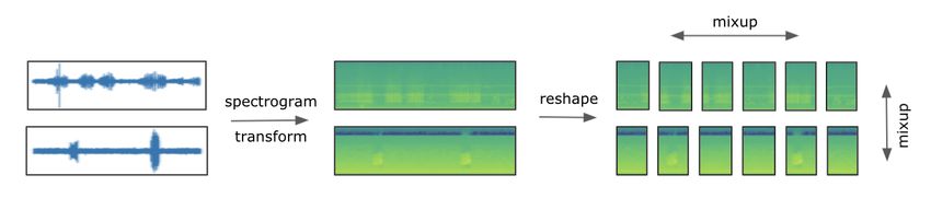
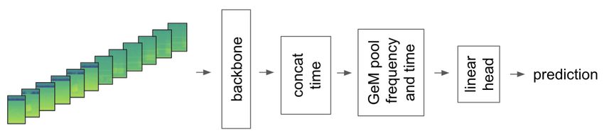
is referred to as CV-3. To receive an even more robust feedback from validation, a bootstrap sampling
method was introduced. Our final validation setup included the following steps:

 • Remove three songs without calls.
 • For k times (e.g., 10) sample 80% of the remaining songs—this should emulate the full test dataset
 (public+private).
 • Apply any kind of threshold selection technique or post processing on this data resembling the
 application in inference for the full public and private test data.
 • For j times (e.g., 50) sample 65% of the remaining songs—this should emulate the private test
 dataset.
 • Calculate the score on each of these j samples.
 • Report average, median, min, max, std scores across all k times j (e.g., 500) subsets

3.2. Modeling
Our final solution is a an ensemble of CNNs which were trained on extracted spectrograms of the
audio clips. Their predictions were further post-processed using a binary CNN for classifying the
presence/absence of avian sound and available meta data with respect to date and region of the test
soundscapes. In the following, we discuss design and training routine of the CNNs. All our models were
trained on GPUs utilizing the Pytorch framework and backbones that were pre-trained on ImageNet and
that are available at timm [11]. In order to perform computational efficient training, we also performed
the spectrogram transformation on GPU using torchaudio3 and mixed precision.

3.2.1. Bird Classifier
The core part of our solution addresses the main task-specific challenges: Firstly, training data is weakly
labeled with bird sound classes being annotated on audio clips of varying length, while prediction needs
to be performed on five second time windows of several minute long recordings. Secondly, due to the
complex soundscapes and broad range of data contributors, the training labels contain a significant
amount of low quality annotations. Lastly, the test data is of significantly different context and of different
quality.

Preprocessing The training data contains short sound clips of different length with weak primary and
secondary labels. To preprocess the training data for modeling, we randomly cropped a 30 second time
window from a recording and applied a mel-spectrogram transformation. Hereby, 30 seconds proved to
be a good compromise between label accuracy and generalization provided by the augmentation. To
account for the five second time window required for inference of the test data, we reshaped the crops
into six parts. Before feeding the spectrograms into the CNN-backbone, we applied a two dimensional
version of mixup [12]. In particular, we not only mixed between different recordings (up to two times),
but also within a recording by mixing the six parts. Our preprocessing was performed on GPU using
functionalities of torchaudio for mel-spectrogram transformation and a custom implementation for
mixup. We illustrate our preprocessing pipeline in Figure 1.

Architecture Given a batch of mel-spectrograms, the model extracts features with a CNN-backbone
pretrained on ImageNet, where in our final solution we used backbones from the resnet [13] efficientnet v2
[14] and nfnet [15] family, which are all available in the timm repository [11]. We re-arrange the tensors
to the 30 second representation by concatenating the respective time segments and use generalized mean
pooling (GeM) [16] of time and frequency dimension before forwarding through a simple one layer head
 3 https://pytorch.org/audio/stable/index.html

Figure 1: Visualization of preprocessing steps for the bird classification model — Input is a 30 second wav crop. After
mel-spectrogram transformation, the input data is split into six equal five second parts, before mixup augmentation
is applied within and between recordings.

Figure 2: Illustration of bird classification model — five second mel-spectrograms are fed into a pretrained CNN-
backbone and re-arranged to 30 second time segments before GeM pooling is applied. A single linear layer outputs
the bird classes.

which results in a prediction of 397 bird classes. For inference we directly fed five second snippets to the
CNN-backbone and applied the head without reshaping. See Figure 2 for an illustration.

Training routine We did not differentiate between primary and secondary labels and set the multilabel
target as the union of both. We trained our models with a binary cross-entropy loss using Adam optimizer
and a 11 to 20 epochs lasting cosine annealing schedule with a batch size varying from 16 to 32 per
model. While the model is not very sensitive to hyperparameters of optimizer and learning rate schedule,
several adjustments lead to significant improvement in classification quality.
 Firstly, we used the quality rating, which is given as meta information for the training data for
weighting a recording’s contribution to the loss. The assumption is that recordings with a lower rating
have worse quality with respect to audio and label and should contribute less to model training. In detail,
we weight each sample by rating/max(ratings).
 Secondly, we used one-sided label smoothing, i.e., adding 0.01 − 0.025 across all negative labels
while positive class is unchanged. This accounts for noisy annotations and absence of birds in “unlucky“
30 second crops. Similar to solutions of past BirdCLEF challenges, we mixed the training data with
additional background noise containing no avian calls. Specifically, we used recordings from the freefield
dataset labeled for bird absence, three recordings of this years validation set containing no bird calls and
30 second crops of past years validation data containing no bird calls according to their annotations; for
details, please refer to Section 2.

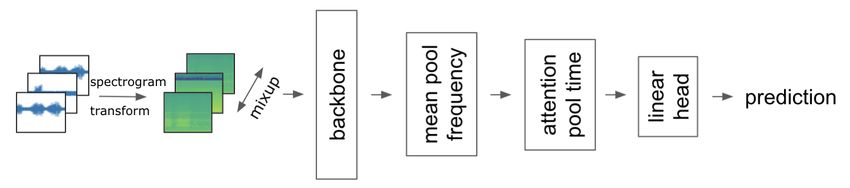
Figure 3: Illustration of binary classification model — Ten second recordings are transformed to spectrograms
before augmented by mixup. Using a pre-trained CNN-backbone features are extracted which are pooled by mean
and attention before a single linear layer outputs a binary bird presence / absence prediction

3.2.2. Binary classifier
A binary classifier was trained to distinguish any bird call from other environment sounds and predictions
were used in the ensembling/post-processing step together with the bird classifier models. For this task,
we only used external data, the binary labeled freefield1010 [7] and BirdVox-DCASE-20k [8] datasets,
both containing ten second audio recordings with or without avian sounds (see Section 2).
 Figure 3 gives an overview of the binary classifier. After transforming the recordings to mel-
spectrograms, mixup augmentation is applied before feeding into a pretrained CNN-backbone. The
output feature map is mean pooled on the frequency axis before applying attention pooling on time
segments. A single linear layer is applied to output a binary bird presence / absence prediction.

3.3. Postprocessing
As F1 metric is evaluated on hard predictions without taking probabilities into account, appropriate
thresholds for detections in a five second segment in soundscapes had to be found. Optimizing the
thresholds on CV-3 and applying it to the test set already indicated good correlation. Nevertheless,
submitting to the public leaderboard with lower thresholds (higher number of predictions) yielded even
better F1 scores. Additionally, one major issue we observed was when blending new models, the threshold
needs to be re-optimized each time. Hard thresholds are not necessarily consistent across models, as
each one can exhibit certain shifts in probabilities and their averages. Consequently, it is challenging to
properly judge if new models work well in an ensemble based on the merit of the models, or only based
on arbitrary probability / threshold shifts that emerged from it. For a more robust approach regarding
shifts in model probabilities, we decided to apply a percentile based thresholding approach. In detail,
we flattened all predictions and calculated the threshold for a certain percentile which we optimized
independently for maximum F1 score on CV-3 and on public leaderboard.
 The more birds a set contains, the lower the percentile should be if predictions are decently ranked.
With this approach, we kept the percentile fixed, thus always predicting the same amount of bird calls,
and just exchanged models, blends and other post processing steps. If the quality in our ranking of
predictions improved, also the score improved.
 On our bootstrapped CV-3, we found a percentile of 0.9987 to be optimal. Based on public leaderboard
feedback, we decided to decrease the percentile a bit further to 0.9981 for our test predictions expecting a
few more birds to be predicted. In retrospective, a slightly higher percentile would have further improved
our solution. By and large, our percentile based thresholding approach appeared to be robust across CV
and LB and generalized well to the unseen private part of the test set.
 Additionally, we employed several smaller post processing steps to improve predictions including: (1)
increasing the probability of birds in songs based on their average prediction probability, (2) smoothing

Figure 4: Visualization of bootstrapped validation results — This figure depicts the distribution of scores over 500
iterations based on our bootstrap validation routine.

neighboring predictions, and (3) we also removed some unlikely predictions based on distance in space and
time given the provided metadata. Additionally, we utilized our binary models predicting whether a bird
song is present in a given window or not and adjusted our predictions by = *(1+ *0.8).
Overall, we fitted 15 binary models and averaged them.

3.4. Ensembling
The ensembling [17] of our models was straightforward since all outputs have the same shapes; we
took the arithmetic mean of the predictions. Post-processing steps (1) and (2) as described in Section 3.3
were applied individually on each model, all other steps were applied after blending. Our final solution
contains nine models differing only on hyperparameters and backbones. Each type of model was fitted
with six different seeds accounting for variability in predictions. Our final inference Kaggle kernel4 ran
only one hour out of three hours allowed giving us further potential room for improvements. In the
following Section 4, we describe according results and go into more detail about the individual models.

4. Results and discussion
As described in Section 3, our final solution is based on an ensemble of multiple models with different
hyperparameter settings and seeds. In Figure 4, we visualize our bootstrapped CV-3 validation results;
the x-axis depicts the score, and the y-axis respective density across all 500 bootstrap iterations. The
distribution exhibits a mean of 0.800, a median of 0.801, a minimum of 0.706, a maximum of 0.906, as
well as a standard deviation of 0.0365. As mentioned, the percentile for validation was set to 0.9987,
while for test we used a percentile of 0.9981. Post-processing parameters are optimized on validation,
and accordingly set for test inference.
 In Table 1, we highlight all individual models as well as the final blend with according settings,
and validation and test scores. For all models, we employed the same thresholding, binary prediction
adjustments, as well as post-processing, meaning that individual results only differ on the trained models
used. Again, note that each individual model averages six different seeds to better account for individual
randomness. For further details please also refer to respective configurations in our code base 5 .
 4 https://www.kaggle.com/ilu000/2nd-place-birdclef2021-inference/
 5 See footnote 1

Table 1
Model results — This table highlights individual model and final ensemble results sorted by CV score. All models
exhibit same postprocessing steps, but differ in utilized backbones and hyperparameters. The main hyperparameter
differences stem from melspec settings, background augmentation, and label smoothing (LS). For melspec settings,
S1 refers to window_size=1024, hop_size=320, fmin=50, fmax=14000, mel_bins=256, power=2, and top_db=80, while
S2 refers to window_size=2048, hop_size=512, fmin=16, fmax=16386, mel_bins=64, power=2, and top_db=None.
 Back
 Model Backbone Melspec LS CV Public LB Private LB
 ground
 ps-6-v2 resnet34 S1 no 0.000 0.7387 0.7649 0.6592
 ps-12-v8 resnet34 S1 yes 0.000 0.7698 0.7665 0.6832
 ps-12-v13 tf_efficientnetv2_m_in21k S2 yes 0.000 0.7716 0.7610 0.6719
 ps-12-v21 eca_nfnet_l0 S2 yes 0.000 0.7803 0.7892 0.6846
 ps-12-v11 tf_efficientnetv2_s_in21k S1 yes 0.000 0.7807 0.7848 0.6751
 ps-12-v30 tf_efficientnetv2_s_in21k S2 yes 0.025 0.7861 0.7841 0.6667
 ch-12-v25a tf_efficientnetv2_s_in21k S2 yes 0.010 0.7901 0.7917 0.6785
 ps-12-v32 tf_efficientnetv2_s_in21k S2 yes 0.010 0.7855 0.7838 0.6656
 ch-12-v25g tf_efficientnetv2_s_in21k S2 yes 0.010 0.7975 0.7869 0.6845
 Ensemble 0.8000 0.7998 0.6893

 The results further highlight the difficulty of robust local validation generalizing well to the unseen
test data. While we can observe a trend of higher CV leading to higher test scores, the best individual
local validation models are not necessarily also the best models on public and private leaderboard scores.
Also, while validation and public LB scores are more aligned, private LB scores exhibit significantly lower
scores even exceeding the lower bounds of our bootstrapped validation scores as shown in Figure 4.
With test data being hidden, we can only speculate that some of the differences can be explained by the
presence of two additional test sites (COL & SNE) for which we can neither robustly judge the presence
/ absence of certain bird species nor the amount of bird segments in respective data strongly driving
absolute scores. It is also unclear, whether public and private test data is split randomly, or based on a
certain logic. However, note that we could gather these insights only after the competition ended, as we
were only able to acquire limited insights into public LB scores (two submissions per day), and no insights
about private LB during competition. Yet, these observations further strengthen the importance of robust
solutions in this competition, that are able to generalize well to partly unseen data and locations.
 While we can observe some (partly random) fluctuations in individual model scores (although each
one consists of six individual seeds), our final ensemble exhibits the best local validation score, best
public LB score, and best private LB score. The ensemble successfully captures the weaknesses and
strengths of each individual model and was a robust choice to generalize well on the unseen test data. A
further testament of the robustness of our solution is given by the fact that we improved our rank on
private leaderboard compared to our initial rank on public leaderboard compared to other contestants.
The final leaderboard results are highlighted in Table 2.

Table 2
Leaderboard results — This table shows the ranking and scores of the top five teams on the private leaderboard
including their respective public leaderboard scores. The team of this article is highlighted in bold.
 Team Public LB Private LB
 Dr.北村愉快仲間 0.7736 (#17) 0.6932 (#1)
 new baseline 0.7998 (#3) 0.6893 (#2)
 Shiro 0.7919 (#4) 0.6891 (#3)
 Third time’s the charm. 0.7897 (#6) 0.6864 (#4)
 Kramarenko Vladislav 0.7897 (#7) 0.6820 (#5)

5. Conclusions
In this work, we discussed how to address challenges of using the crowd-sourced dataset xeno-canto for
productive bird sound recognition as part of the second place solution to BirdCLEF2021 [1]. Specifically,
we showed how to efficiently finetune a pre-trained CNN with weakly labeled data by reshaping input
and output tensors and how to handle noisy labels by using quality rating, as well as label smoothing.
Furthermore, we demonstrated that mixing train dataset recordings internally as well as with external
data significantly improves generalization to distinct acoustic environments. Thus, we gave suggestions
to enhance autonomous monitoring of avian population which is essential for assessing the biodiversity
and healthiness of ecosystems and a sustainable development of humanity.

Acknowledgments
We would like to thank Kaggle and the competition hosts for conducting this interesting competition as
well as all other competitors on Kaggle for the challenge. Additionally, a big thank you goes to all users
of xeno-canto generously uploading and sharing their bird recordings with the world. Without them
this work would not have been possible.

References
 [1] S. Kahl, T. Denton, H. Klinck, H. Glotin, H. Goëau, W.-P. Vellinga, R. Planqué, A. Joly, Overview of BirdCLEF 2021: Bird call
 identification in soundscape recordings, in: Working Notes of CLEF 2021 - Conference and Labs of the Evaluation Forum,
 2021.
 [2] A. Joly, H. Goëau, S. Kahl, L. Picek, T. Lorieul, E. Cole, B. Deneu, M. Servajean, R. Ruiz De Castañeda, I. Bolon, H. Glotin,
 R. Planqué, W.-P. Vellinga, A. Dorso, H. Klinck, T. Denton, I. Eggel, P. Bonnet, H. Müller, Overview of LifeCLEF 2021: a
 system-oriented evaluation of automated species identification and species distribution prediction, in: Proceedings of the
 Twelfth International Conference of the CLEF Association (CLEF 2021), 2021.
 [3] H. Goëau, P. Bonnet, A. Joly, Overview of PlantCLEF 2021: cross-domain plant identification, in: Working Notes of CLEF
 2021 - Conference and Labs of the Evaluation Forum, 2021.
 [4] L. Picek, A. M. Durso, R. Ruiz De Castañeda, I. Bolon, Overview of SnakeCLEF 2021: Automatic snake species identification
 with country-level focus, in: Working Notes of CLEF 2021 - Conference and Labs of the Evaluation Forum, 2021.
 [5] T. Lorieul, E. Cole, B. Deneu, M. Servajean, A. Joly, Overview of GeoLifeCLEF 2021: Predicting species distribution from 2
 million remote sensing images, in: Working Notes of CLEF 2021 - Conference and Labs of the Evaluation Forum, 2021.
 [6] X. canto Foundation, xeno-canto, https://www.xenocanto.org, 2021.
 [7] D. Stowell, M. D. Plumbley, freefield1010 - an open dataset for research on audio field recording archives, in: Proceedings of
 the Audio Engineering Society 53rd Conference on Semantic Audio (AES53), Audio Engineering Society, 2014.
 [8] V. Lostanlen, J. Salamon, A. Farnsworth, S. Kelling, J. P. Bello, Birdvox-full-night: a dataset and benchmark for avian flight
 call detection, in: Proc. IEEE ICASSP, 2018.
 [9] D. Stowell, Y. Stylianou, M. Wood, H. Pamuła, H. Glotin, Automatic acoustic detection of birds through deep learning:
 the first bird audio detection challenge, Methods in Ecology and Evolution (2018). URL: https://arxiv.org/abs/1807.05812].
 arXiv:1807.05812.
[10] S. Kahl, M. Clapp, W. Hopping, H. Goëau, H. Glotin, R. Planqué, W.-P. Vellinga, A. Joly, Overview of BirdCLEF 2020: Bird
 sound recognition in complex acoustic environments, in: CLEF 2020, 2020.
[11] R. Wightman, Pytorch image models, https://github.com/rwightman/pytorch-image-models, 2019. doi:10.5281/zenodo.
 4414861.
[12] H. Zhang, M. Cisse, Y. N. Dauphin, D. Lopez-Paz, mixup: Beyond empirical risk minimization, arXiv preprint arXiv:1710.09412
 (2017).
[13] K. He, X. Zhang, S. Ren, J. Sun, Deep residual learning for image recognition, 2015. arXiv:1512.03385.
[14] M. Tan, Q. V. Le, EfficientNetV2: Smaller models and faster training, 2021. arXiv:2104.00298.
[15] A. Brock, S. De, S. L. Smith, K. Simonyan, High-performance large-scale image recognition without normalization, 2021.
 arXiv:2102.06171.
[16] F. Radenović, G. Tolias, O. Chum, Fine-tuning CNN image retrieval with no human annotation, 2018. arXiv:1711.02512.
[17] L. K. Hansen, P. Salamon, Neural network ensembles, IEEE transactions on pattern analysis and machine intelligence 12
 (1990) 993–1001.