Report of the Ad-hoc Group on the Impacts of Sonar on Cetaceans and Fish (AGISC) - (2nd edition)
←
→
Page content transcription
If your browser does not render page correctly, please read the page content below
ICES AGISC 2005
       ICES Advisory Committee on Ecosystems
                       ICES CM 2005/ACE:06

Report of the Ad-hoc Group
 on the Impacts of Sonar on
Cetaceans and Fish (AGISC)
                      (2nd edition)

                  By correspondence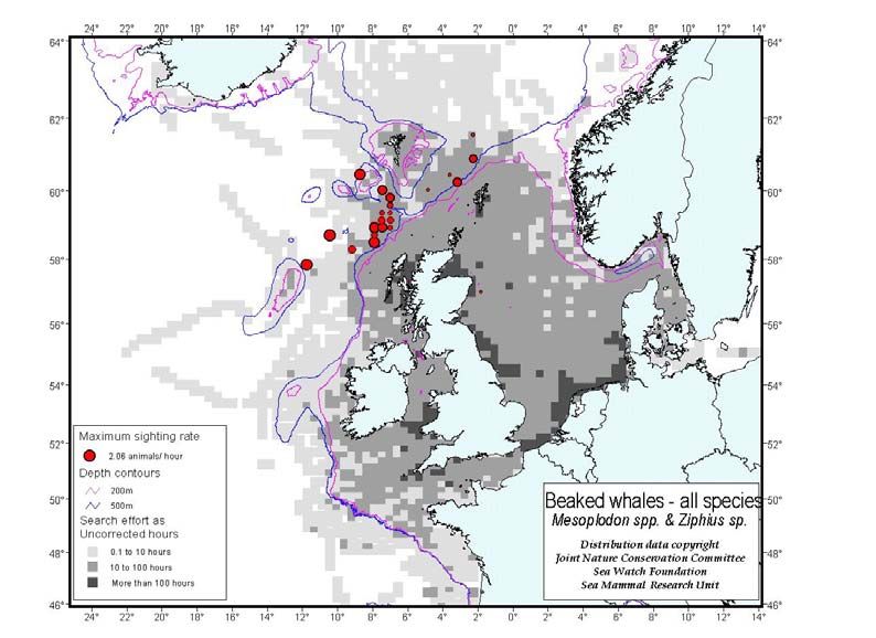
International Council for the Exploration of the Sea
Conseil International pour l’Exploration de la Mer
H.C. Andersens Boulevard 44-46
DK-1553 Copenhagen V
Denmark
Telephone (+45) 33 38 67 00
Telefax (+45) 33 93 42 15
www.ices.dk
info@ices.dk

Recommended format for purposes of citation:
ICES. 2005. Report of the Ad-hoc Group on Impacts of Sonar on Cetaceans and Fish
(AGISC) CM 2006/ACE:06 25pp.

For permission to reproduce material from this publication, please apply to the General
Secretary.

The document is a report of an Expert Group under the auspices of the International Council
for the Exploration of the Sea and does not necessarily represent the views of the Council.
© 2005 International Council for the Exploration of the Sea
ICES AGISC report 2005, 2nd edition                                                                                                          | i

Contents
    1    Introduction ................................................................................................................................... 1
         1.1      Participation........................................................................................................................... 1
         1.2      Terms of Reference ............................................................................................................... 1
         1.3      Justification of Terms of Reference....................................................................................... 1
         1.4      Framework for response ........................................................................................................ 2
         1.5      Overview by the chair............................................................................................................ 2
         1.6      Acknowledgements ............................................................................................................... 3

    2    Physical background ..................................................................................................................... 4
         2.1      The nature of sound ............................................................................................................... 4
         2.2      Units for measuring sound..................................................................................................... 4
                  2.2.1 Use of the decibel scale in water............................................................................... 4
         2.3      Parameters for estimating noise............................................................................................. 4
                   2.3.1 Source level .............................................................................................................. 5
                   2.3.2 Impulsive sound........................................................................................................ 5
                   2.3.3 Sound propagation and transmission loss ................................................................. 6
         2.4      Ambient noise........................................................................................................................ 7
         2.5      Sonar in general ..................................................................................................................... 8
                   2.5.1 Low-frequency sonar ................................................................................................ 8
                   2.5.2 Mid frequency sonar ................................................................................................. 9
                   2.5.3 High frequency sonar................................................................................................ 9

    3    Biological Background - Cetaceans............................................................................................ 10
         3.1      Hearing in cetaceans............................................................................................................ 10
                  3.1.1 Anatomy and physiology ........................................................................................ 10
                  3.1.2 Hearing in smaller odontocetes............................................................................... 11
                  3.1.3 Hearing in mysticetes ............................................................................................. 12
         3.2      Potential effects of sound on cetaceans ............................................................................... 12
                   3.2.1 Direct damage to hearing........................................................................................ 12
                   3.2.2 Non-auditory tissue damage ................................................................................... 13
                   3.2.3 Masking and changes in vocal behaviour ............................................................... 15
                   3.2.4 Behavioural reactions ............................................................................................. 16

    4    Cetaceans and sonar.................................................................................................................... 17
         4.1      Marine mammals ................................................................................................................. 17
         4.2      Beaked whales ..................................................................................................................... 17
                   4.2.1 Review of literature on effects of sonar on beaked whales..................................... 20
                   4.2.2 Case study: Greece ................................................................................................. 22
                   4.2.3 Case study: Bahamas .............................................................................................. 25
                   4.2.4 Case study: Canary Islands ..................................................................................... 27
         4.3      Other cetaceans and sonar ................................................................................................... 28
                  4.3.1 Research on LFA and cetaceans ............................................................................. 28

    5    Mitigation measures for cetaceans ............................................................................................. 29
         5.1      Introduction ......................................................................................................................... 29
         5.2      Control at source.................................................................................................................. 30
         5.3      Mitigation of death and injury caused by the direct effects of sound .................................. 30
                  5.3.1 Marine Mammal Observers (MMOs) ..................................................................... 31
ii |
5.3.2 Passive Acoustic Monitoring (PAM) or Active Acoustic Monitoring
(AAM) .................................................................................................................... 31
5.4 Other control methods ......................................................................................................... 31
5.4.1 Scheduling .............................................................................................................. 31
5.4.2 Warning signals ...................................................................................................... 32
5.5 Monitoring........................................................................................................................... 32
5.5.1 Noise monitoring .................................................................................................... 32
5.5.2 Marine mammal observation .................................................................................. 32
5.6 Mitigation measures in use for military sonars with regard to marine mammals ................ 33
5.6.1 Guidelines for sonar research testing by NATO and marine mammal
risk mitigation research at the NATO Undersea Research Centre.......................... 33
5.6.2 Mitigation on UK naval vessels or in UK sonar tests ............................................. 33
5.6.3 Mitigation on Australian naval vessels ................................................................... 35
5.6.4 Mitigation on Italian naval vessels ......................................................................... 35
5.6.5 Mitigation on US naval vessels during training and during exercises .................... 36
5.6.6 Future mitigation development ............................................................................... 36
6 Summary of gaps in understanding for marine mammals....................................................... 36
7 Other relevant items.................................................................................................................... 37
7.1 Noise pollution as a more serious problem? ........................................................................ 37
8 General conclusion for marine mammals.................................................................................. 38
9 Fish 40
9.1 Biological background......................................................................................................... 40
9.1.1 Hearing in fish ........................................................................................................ 40
9.1.2 Impact of sonar on fish ........................................................................................... 45
9.1.3 Mitigation measures for fish ................................................................................... 47
10 Recommendations........................................................................................................................ 47
10.1 Future investigations and research for marine mammals..................................................... 47
10.2 Future research on fish and sonar ........................................................................................ 48
11 References .................................................................................................................................... 48ICES AGISC report 2005, 2nd edition | 1
1 Introduction
This is the second edition of our report. A first edition, covering effects on physical
background, sonar usage and effects and mitigation in relation to marine mammals was
produced early in 2005. This second edition contains improved sections on physical
background and mitigation for marine mammals, and an entirely new section on fish.
1.1 Participation
The following members of the Ad hoc Group on the Impact of Sonar on Cetaceans and Fish
(AGISC) participated in producing this report (see Annex 1 for addresses).
Tony Hawkins UK
Finn Larsen Denmark
Mark Tasker (chair) UK
Chris Clark USA
Antonio Fernández Spain
Alexandros Frantzis Greece
Roger Gentry USA
Jonathan Gordon UK
Tony Hawkins UK
Paul Jepson UK
Finn Larsen Denmark
Jeremy Nedwell UK
Jacob Tougaard Denmark
Peter Tyack USA
Tana Worcester Canada
1.2 Terms of Reference
At the MCAP meeting January 2004, an Ad hoc Group on the Impact of Sonar on Cetaceans
and Fish (AGISC) was established and was given the following terms of reference:
i. Review and evaluate all relevant information concerning the impact of sonar on
cetaceans and fish;
ii. Identify the gaps in our current understanding;
iii. Prepare recommendations for future investigations and research;
iv. Prepare draft advice on possible mitigation measures to reduce or minimize the
impact of sonar on cetaceans and fish.
1.3 Justification of Terms of Reference
The terms of reference derive from a letter from Catherine Day (Director General of EC DG
Environment) to David Griffith (General Secretary, ICES), dated 25 September 2003. In this
letter, the European Commission indicated that it had for some time received complaints about
the impact of sonar on marine mammals. These complaints claimed that the emission of
intense, low and medium frequency tone bursts has a disturbing effect on cetaceans.
Information had also been forwarded indicating that these sonars might have an impact on fish
and fish behaviour.
European legislation (mainly the Habitats Directive (92/43/EC)) requires Member States of
the European Union to take measures to establish a system of strict protection for all cetaceans
in European waters. The European Commission does not have a comprehensive and2 | ICES AGISC report 2005, 2nd edition
authoritative review of information concerning the impact of sonar, and thus finds it difficult
to develop a clear position on the issue.
The Commission therefore asked ICES to undertake a scientific review and evaluation of
relevant information concerning the impact of sonar on cetaceans and fish, to identify the gaps
in current understanding and to make recommendations for future investigations or research.
The Commission is also interested in advice on possible mitigation measures to reduce or
minimise the impact of sonar on cetaceans and fish.
1.4 Framework for response
The Group’s response to these terms of reference has been compiled by correspondence.
Sections were initially drafted by Group Members and then agreed by circulation to all
members. Much of the report is based on existing review literature (not all relating to sonar
directly), updated and amended as appropriate.
1.5 Overview by the chair
The effects of human inputs to natural systems have been a topic of interest and study for
many years, however much the greatest amount of work has been carried out on chemical
inputs, both in the form of contaminants and nutrients. The subject of energy input has
historically received much less attention. The anthropogenic input of sound to the marine
environment started with the coming of mechanically propelled ships, but until the advent of
sonar, nearly all sound input was a by-product of another activity as opposed to deliberate.
Both forms of input though carry the risk of affecting other marine life. Evidence has been
available for some time that anthropogenic noise has the capacity to disturb those forms of
marine life dependent on sound for communication and sensing in the seas. Much less
evidence has been available on damage, injury or lethal consequences at the individual level,
and none at the population level. A series of incidents in recent years when certain deep-
diving whale species stranded or died co-incident with the use of high-powered sonar alerted
many more to the risks posed by sound. Research elsewhere indicated that other forms of loud
sound might affect fish.
The behaviour of sound in the marine environment is complex and is equally complex to
describe. We have attempted to describe the physical background briefly in the first main part
of this report, but are aware that this may be too brief and simplistic for some. We refer those
readers to standard texts for further information. This section includes a brief description of
the types of sonar in use today. It proved difficult to find information on the characteristics of
many forms of sonar.
The next section of the report deals with the mechanisms for hearing in cetaceans and
describes the potential effects of sound on these mechanisms and the behaviour of these
animals. Until recently, most concern has focussed on the effects on hearing and
communication systems of cetaceans but recent evidence is indicating that damage may also
be caused through other mechanisms, and perhaps indirectly through dangerous alterations in
behaviour. There is however little experimental evidence currently in the public domain of the
effects of sonar on the acoustic systems, physiology or behaviour of cetaceans. Logistically,
any such experiments are easiest to conduct in the laboratory on individual animals, but
extrapolating the few available items of information to wild populations is at present very
difficult and uncertain.
Section 4 reviews observations and deductions from cases where whales have stranded or
been found dead in association with the nearby use of military sonar. As with many
observational cases, obtaining the best and most pertinent evidence proved difficult both from
the corpses and in other cases of strandings, from the military authorities. In order to improveICES AGISC report 2005, 2nd edition | 3
deductions, we ideally need to complete three of four cells in a 2 x 2 matrix - naval operations
occurred or not occurred versus marine mammal strandings occurred or not occurred. We have
knowledge of some stranding events associated with naval operations, and possibly some
information on the number of stranding events without naval sonar being present, but we do
not know how many naval sonar operations occurred (in suitable beaked whale habitat)
without any observed marine mammal strandings. It is though agreed that high-powered, mid-
frequency sonar can affect beaked whales in particular. These effects can lead to death, either
at sea or as a consequence of stranding ashore. These effects may be caused by a lethal
behavioural change leading to physiological damage, or possibly by direct physiological
damage. Hypotheses exist to explain these effects. It seems likely that these effects also occur
at lower received sound levels than previously thought likely to cause damage and as a
consequence the sphere of effect of these sonars is not known. Coupled with the lack of
knowledge of the population size or distribution of beaked whales, we cannot be certain of
whether population level effects might occur. However, at present it appears that these
military sonars are not used widely. This could change in the future if these sonars were more
widely deployed on ships or were used in non-exercise situations. Effects would be most
severe in areas important for beaked whales.
Section 5 provides an overview of possible measures to mitigate the effects of sonar on marine
mammals as well a brief description of the measures being undertaken by some the Navies of
some nations in relation to military sonar.
Section 6 outlines some of the gaps in understanding around this issue and makes some
suggestions as to how they might be addressed. Section 7 notes that other facets of the issue of
noise in the ocean could have potentially more significant effects than direct lethal effects on
individuals. In particular, the apparently increasing levels of anthropogenic low-frequency
noise (mostly from shipping) may have consequences for the large baleen whales that use
these frequencies for communication. General conclusions on marine mammals are
summarised in Section 8
Section 9 describes relevant aspects of fish biology and the potential impact of sound,
particularly sonar, on fish. There are very few studies of this and it should be noted that those
studies cannot be regarded as being representative of the wide diversity of fish species that
occur in the oceans. Effects of sonar have been noted at the individual level. Despite this,
wide-ranging species of fish of commercial importance are unlikely to be affected at the
population level with current rates of usage (and areas of usage) of military sonar. Other
sonars (and noise sources) are more widespread. Research is suggested on the more subtle and
on the cumulative effects of noise on fish.
Section 10 provides the groups recommendations that may form the basis of advice from
ICES.
1.6 Acknowledgements
We thank Rene Swift and Jay Barlow for help in accessing some of the references used in this
report. Gerald D'Spain, Jim Miller, and Dave Bradley provided comments on noise budgets.
Bertel Møhl and Hans Lassen both provided helpful comments. Jake Rice read the whole
report and provided many helpful comments. We thank John Polglaze, Mike Carron, Fernando
Cerrutti, and Claire Burt for comments on the chapter on mitigation. Thanks to Arthur Popper
for providing an update on his work on SURTASS LFA sonar and fishes. Jake Rice and
Håkan Westerberg are thanked for more general comments.4 | ICES AGISC report 2005, 2nd edition
2 Physical background
2.1 The nature of sound
Sound consists of a symmetrical fluctuation in pressure around the hydrostatic pressure,
accompanied by a back and forth motion of the component particles of the medium. For a
plane wave travelling in open space without any interaction with objects or boundaries, the
relationship between sound pressure (p) and particle velocity (v) is p = (ρc)v, where ρ (kg/m3)
is the density of the medium and c (m/s) is the speed of sound in the medium. The acoustic
energy flux or intensity (I) of a sound wave is the product of the pressure multiplied by the
particle velocity, and has the units of Joule per square meter per second (J/m2-s) or watts per
square meter (W/m2). For a plane wave the intensity (or energy flux) is given by I = p2/(ρc). It
is equivalent to the amount of energy in Joules passing through a unit area per unit time as the
sound wave travels unbounded in the medium.
2.2 Units for measuring sound
Underwater sound is usually expressed using the logarithmic decibel (deciBel) scale.
Underwater sound is conventionally presented in decibels referenced to 1 microPascal, i.e. as
dB re 1 µPa, and this convention has been adhered to in this report.
2.2.1 Use of the decibel scale in water
The fundamental unit of sound pressure is the Newton per square metre, or Pascal. However,
when describing underwater acoustic phenomena it is normal to express the sound pressure
through the use of a logarithmic scale termed the Sound Pressure Level. There are two reasons
for this. First, there is a very wide range of sound pressures measured underwater, from
around 0.0000001 Pa in quiet sea to around 10,000,000 Pa for an explosive blast. The use of a
logarithmic scale compresses the range so that it can be easily described (in this example,
from 0 dB to 260 dB re 1 µPa). Second, many of the mechanisms affecting sound underwater
cause loss of sound at a constant rate when it is expressed on the dB scale.
The Sound Pressure Level (SPL) is defined as: SPL = 20 log (P/Pref)
where P is the sound pressure to be expressed on the scale and Pref is the reference pressure,
which for underwater applications is 1 µPa. For instance, a pressure of 1 Pa would be
expressed as an SPL of 120 dB re 1 µPa.
2.3 Parameters for estimating noise
In order to provide an objective and quantitative assessment of degree of any environmental
effect it is necessary to estimate the sound level as a function of range. To estimate the sound
level as a function of the distance from the source, and hence the range within which there
may be an effect of the sound, it is necessary to know the level of sound generated by the
source and the rate at which the sound decays as it propagates away from the source. These
two parameters are:
• the level of sound generated by the source or Source Level (SL) and
• the rate at which sound from the source is attenuated as it propagates or Transmission
Loss (TL)
These two parameters allow the sound level at all points in the water to be specified, and in
the current state of knowledge are generally best measured directly at sea, although acoustical
models exist which may give reasonably reliable results for propagation from sonar systems inICES AGISC report 2005, 2nd edition | 5 homogeneous deep water. However, these data have usually to be extrapolated to situations other than those in which the noise was measured; in these cases the commonest method of modelling the level is from the expression: Received Level (RL) = SL-TL Conventionally, the RL is calculated in dB re 1 μPa, but a similar expression may be used to estimate the received level of other measures of sound such as its impulse. Note that both RL and SL are absolute values, while TL is a rate. If the level of sound at which a given effect of the sound is known, an estimate may be made of the range within which there will be an effect. Sound can behave in very different ways in shallow water compared with deep water and is therefore much more difficult to model. 2.3.1 Source level The Source Level of a source is defined as the level of sound at a nominal distance of 1m, expressed in dB re 1 μPa. However, there are several assumptions implicit in this definition. Sound is composed not just of sound pressure but also a motion of the component particles of the medium (particle velocity). In the area very close to the sound source (the near field) there are very large particle motions for a given sound pressure and this has implications for organisms sensitive to particle motion – such as many fish, but less so for cetaceans. However, this area is very small (a few metres at the greatest) so population level effects are extremely unlikely and even effects on individuals would not be frequent. In addition, some sound sources, such as airgun arrays or steerable sonars, are composed of several sound sources that are operated simultaneously. When one is within several times the diameter of the source(s) the sound field is variable. It is therefore good practice to measure the sound pressure in the far field, at sufficient distance from the source that the effects of particle motion and complexities of multiple sound sources close together have reduced, and to use this pressure to estimate the apparent level at a nominal 1m from the source. However, this apparent level may not predict the actual level at ranges near an array of sources. An array of sources each of which operates at one particular source level may have a higher apparent source level far from the array. However as an animal approaches the array, it is unlikely that it would experience a sound level greater than one of the individual sources from which the array is made up. A ‘measurement’ of the apparent level can be made by assuming inverse dependence of pressure on the range, R, from the noise source, or by extrapolating the far field pressure. There is in general no reliable way of predicting the noise level from sources of man-made noise, and hence it is normal to measure the Source Level directly when a requirement exists to estimate far-field levels. 2.3.2 Impulsive sound Powerful impulsive sounds are generated by the use of explosives underwater, by the airgun arrays used in seismic surveying, and by some forms of construction activity such as underwater pile driving. These sources generate impulsive waves of short duration, high peak pressure, and a wide frequency bandwidth, and may consequently have an effect on marine organisms. Historically, two key parameters have been used to describe the severity of an impulsive source, the peak pressure and the impulse. The peak pressure of a blast wave Pmax is the maximum level of overpressure, that is, the pressure above the local ambient pressure caused by the sound. This is usually at the initial peak of the waveform and is easily read from a recording of the sound. The impulse I is defined as the integral of pressure over time and is given by
6 |                                                                ICES AGISC report 2005, 2nd edition

            ∞
      I = ∫ P(t )δt
            0

      where I is the impulse in Pascal-seconds (Pa.s), P(t) is the acoustic pressure in Pa of the blast
      wave at time t and t is time. Impulse may be thought of as the average pressure of the wave
      multiplied by its duration. The importance of impulse is that in many cases a wave acting for a
      given time will have the same effect as one of say twice the pressure acting for half the time.
      The impulse of both these waves would be the same.

      Several workers (Johnstone, 1985; Ross et al., 1985; Larsen and Johnsen, 1992) have showed
      the impulse of the shock wave (Yelverton et al., 1975) to be the best predictor of damage to
      fish and other aquatic animals from explosives. However, this measure tends to give
      conservative estimates for shallow water (5-10m depth) and is not considered suitable in areas
      having hard, reflective beds or under ice (Engelhardt et al., 1985).

      The sound duration as well as the sound level is important in estimating the damage that may
      be caused by a sound. To compare sound events of varying duration and intensity the SEL or
      Sound Exposure Level (in dB) may be determined by converting the total noise energy
      measured during a noise event to an equivalent dB level for a single event that would be only
      one second in duration. The SEL accounts for both the magnitude and the duration of the
      noise event. The SEL may be calculated by summing the cumulative pressure squared (p2)
      over time and is expressed as dB re 1µPa2-s. Yet another method of quantifying the noise
      environment is to determine the value of a steady-state sound that has the same sound energy
      as that contained in the time-varying sound. This is the Equivalent Sound Level (Leq).

      It is important when measuring impulsive sounds to record examples of the waveforms, so
      that alternative metrics may later be applied.

      2.3.3 Sound propagation and transmission loss

      The level of a sound diminishes as it spreads out from its source. A sound of 230 dB one
      metre from the source drops to 224 at 2m, 218 at 4 m, 212 at 8m out to 190 dB at 100m if the
      medium is homogeneous out to 100m. The reason for this extensive loss is that the energy
      emanating from the source expands in all directions, spread over a sphere of ever-increasing
      volume. This is called spherical spreading.

      Sound consists not only of a variation in pressure, but also of a back and forth motion of the
      medium. While sounds are normally monitored by measuring the sound pressure, many fish
      respond to the particle motion (measured as the particle velocity, particle displacement or
      particle acceleration). As we have seen in section 2.1, in a free sound field the particle
      velocity can readily be estimated from the sound pressure. However, close to a source, in the
      ‘near field’, much larger particle velocities are associated with a given sound pressure.
      Estimating the changes in particle motion with distance from a source depends on the nature
      of the source. Note that the ‘near field’ can be quite extensive (extending for several metres)
      for low-frequency sound.

      Losses far from the source are complex and depend on the depth of water, temperature,
      salinity and other factors. Not all frequencies propagate equally. High frequency sounds have
      a short wavelength and are absorbed by seawater, reflected by material in the water and
      converted to heat faster than low frequency sounds that have a long wavelength. For that
      reason, low frequency sounds propagate farther than a high frequency sound of the same
      source level. However, even though they propagate further, their levels continually decrease
      through spreading loss. These effects may be different in very shallow water, when low
      frequencies can attenuate faster than high frequencies.

      Sound rarely spreads out uniformly. The path that sound takes through water is affected by the
      presence of a reflecting bottom and surface, and by factors that change water density, mainly
ICES AGISC report 2005, 2nd edition | 7
temperature, salinity, and depth. Thus for instance, a sound produced near the surface over
deep water in summer could to dive immediately toward the bottom where, because of
pressure, it turns and rises, reaching the surface some 30 km away. It could continue this
diving and rising in a pattern called convergence zone propagation. In the winter, the same
sound would tend to stay near the surface because propagation conditions prevent the sound
from reaching great depth. If the water is very shallow, sound bounces between the surface
and bottom and decreases close to shore. The relevance for marine mammals is that the
exposure they receive from a human source is very variable and depends not only on distance
from the source and frequency, but their depth, the depth of the water, and the time of year.
Sound propagation over long ranges in the ocean is therefore relatively unpredictable and
cannot be influenced by man. Sound may also travel horizontally through the seabed, re-
emerging back into the water at a distance. Refraction and absorption further distort the
impulse, leading to a complex wave arriving at a distant point that may bear little resemblance
to the wave near the source. Finally, sound may be carried with little loss to great distance by
being trapped by reflection and refraction between layers of water at different densities in the
water column (sound channels). Sound propagating in a channel is said to have cylindrical
spreading. Predicting the level of sound from a source is therefore extremely difficult, and use
is generally made of simple models or empirical data based on measurements for its
estimation.
2.4 Ambient noise
Background, or ambient, noise occurs in all oceans and seas. There are many sources of
ambient noise that may be classified as either:
• physical - wind driven, turbulence, seismic (earthquakes etc) and microseisms,
thermal, rainfall, seabed generated and icebergs;
• biological - animal sounds and movement;
• man-made - shipboard machinery, propeller, water flow around, and discharges from,
the hull.
These diverse sources all contribute to the generation of background noise levels but the
ambient level is not the result of noise sources alone; it also depends on propagation
conditions and the absorption of sound in seawater (Francois and Garrison, 1982).
Wenz (1962) and Urick (1986) describe levels of ambient noise in the ocean. The level of
ambient noise in the sea increases continuously as the lower frequencies, below about 50 kHz,
are approached. In the northern hemisphere, from 200 Hz to 10 Hz shipping noise is dominant.
In the southern hemisphere, this band is less dominated by shipping. In both hemispheres there
is considerable variation, with maximum ambient noise in this band being close to major
shipping lanes.
Overall trends of the level of sounds in the sea can be broken down into anthropogenic and
non-anthropogenic components. For instance, there is evidence that global climate change
may have resulted in higher sea states (Bacon and Carter, 1993; Graham and Diaz, 2001),
which would increase ambient noise levels. Over the past few decades, however, it is likely
that increases in anthropogenic noise have been more prominent. In order of importance
viewed on a global scale, the anthropogenic sources most likely to have contributed to
increased noise are commercial shipping, offshore oil and gas exploration and drilling, and
naval and other uses of sonar.
Ross (1987; 1993) suggested that ambient sound levels have increased by 10 dB or more
between 1950 and 1975. These trends are most apparent in the eastern Pacific and eastern and
western Atlantic, where they are attributed to increases in commercial shipping. Ross (1993)
assumed that a doubling of the number of ships explained 3 to 5 dB, and greater average ship8 | ICES AGISC report 2005, 2nd edition
speeds, propulsion power, and propeller tip speeds explained an additional 6 dB. However,
recent work (Wales and Heitmeyer, 2002) calls some of these indices into question.
Only one actual measurement of long-term trends in ocean noise is available, and for only one
site in the oceans. Andrew et al. (2002) used the same U.S. Navy acoustic array used by Wenz
(1969) to make modern recordings. A low frequency noise increase of 10 dB over 33 years
was observed at a site off the central California coast. The explanation for a noise increase in
this band is the growth in commercial shipping, in terms of both number of ships and gross
tonnage. From 1972 to 1999, the total number of ships in the world’s fleet increased from
approximately 57,000 to 87,000, and the total gross tonnage increased from 268 to 543 million
gross tons. This increase probably is not representative of the oceans as a whole because
shipping density differs regionally.
Mazzuca (2001) compared the results of Wenz (1969), Ross (1987), and Andrew et al. (2002)
to derive an overall increase of 16 dB in low-frequency noise from 1950 to 2000. This
corresponds to a doubling of noise power (3 dB) every decade for the past five decades,
equivalent to a 7 percent annual increase in noise. During this period the number of ships in
the world fleet tripled (from 30,000 to 87,000) and the gross tonnage increased by a factor of
6.5 (from 85 to 550 million gross tons) (National Research Council, 2003 from McCarthy and
Miller, 2002).
A noise budget that covers both anthropogenic and natural sources of noise would be of
considerable interest. However, no single noise budget provides a complete assessment of the
potential impact of man-made sound on the marine environment. For example, a noise budget
can be created that is based only on the characteristics of the source, e.g. source level, so that
propagation effects are not taken into account. If, on the other hand, received sound levels are
the property of interest, the relative contribution of mid frequency (1 kHz - 10 kHz) sources
such as Navy hull-mounted sonar would be significantly reduced with respect to low
frequency sources because of the ocean's selective absorption of high frequency sounds,
discussed above. For example, mid frequency sonar operating at 235 dB re 1 μPa @ 1 m in the
Bahamas event (see Section 4.2.3) was barely detectable by an acoustic range 160 km away,
but airguns operating at comparable source levels were detectable over thousands of km
(Nieukirk et al., 2004). In addition, since military sonars operate in a few specific areas at any
given time, they probably could not be discerned in a comprehensive global noise budget in
which the received sound was averaged over space and time. Therefore, local as well as global
noise budgets should be constructed, particularly for critical marine mammal habitats. A
further step would be to create noise budgets that take account of the auditory capabilities of
various groupings of marine organisms (odontocetes such as beaked whales, large baleen
whales, specific fish or groups of fish etc).
2.5 Sonar in general
Active sonar is the use of acoustic energy for locating and surveying. Sonar was the first
anthropogenic sound to be deliberately introduced into the oceans on a wide scale. There is a
variety of types of sonars that are used for both civilian and military purposes. They can use
all sound frequencies and can be conveniently categorised into low (10 kHz). Military sonars use all frequencies, while civilian sonar
uses some mid but mostly high frequencies.
2.5.1 Low-frequency sonar
Low frequency sonars are used by navies for long-range (in the order of a few hundred
kilometres) surveillance. For example, the US Navy has developed the SURTASS-LFA
(Surveillance Towed Array Sensor System – Low Frequency Active) system that uses a
vertical array of 18 projectors using the 100-500 Hz frequency range. The source level of eachICES AGISC report 2005, 2nd edition | 9 projector is approximately 215 dB re 1 μPa @ 1m and the ‘ping’ length is 60 to 100 sec (Johnson, 2001). Over the last few years, this system has only been used on a limited number of occasions, and is now regularly used in military testing or exercises. Many other countries of the world are developing low frequency sonar (Pengelly and Scott, 2004) to detect quiet diesel-electric submarines. 2.5.2 Mid frequency sonar Military mid frequency sonars are used to survey areas tens of kilometres in radius and are used to find and track underwater targets. A US Navy hull-mounted system (AN/SQS-53C) sonar system uses pulses in the 2 – 10 kHz range (normally 3.5 kHz) and has operated at 235 dB re 1 μPa @ 1m with ping lengths of about 2.5 sec. Another system (AN/SQS-56) uses this same frequency band but with lower source levels (223 dB re 1 μPa @ 1m) (Evans and England, 2001). Similar mid-frequency sonars are used by many navies of the world, including the Spanish navy during the Canary Islands event (see Section 4.2.4). Most usage of these systems has been confined to comparatively well-defined exercise areas, which make up a small proportion of the world’s oceans. Even in these areas, activity times are relatively short and episodic, and propagation distances are small because of the frequencies involved. In addition, only a small proportion of the world’s military ships carry these sonar systems. These systems were formerly used for antisubmarine work in open water, but are now most often used in coastal areas, submarine canyons or other choke points where quiet diesel- electric submarines may hide within acoustic clutter. Some non-military sonars also operate in this frequency band. Bathymetric sonars use these frequencies for wide-area, low resolution surveys. The Fugro Seafloor survey model SYS09 for instances uses both 9 and 10 kHz transducers operated at 230 dB re 1 μPa @ 1m. Sub- bottom profilers typically use 3.5 kHz transducers operated at source levels of 204 dB re 1 μPa @ 1m. The regional resolution GLORIA survey sonar uses 6-7 kHz band (no source level published). 2.5.3 High frequency sonar Military high-frequency sonars are either used in attacking (mines or torpedoes) or defending (mine countermeasure, anti-torpedo) systems and are designed to work over hundreds of metres to a few kilometres. These sonars use a wide range of modes, signal types and strengths. As with other military sonars, their usage is generally confined to exercise areas, except when they are used for commercial-like uses such as depth sounding. Fish finders and most commercial depth sounders operate at high frequencies. Usually, but not always, they project a lower power signal and have narrower beam patterns and shorter pulse lengths (a fraction of a second) than military sonars. These systems cannot be used at shallow depths at high powers due to cavitation (Urick, 1975). Most of the systems focus sound downwards, though some horizontal fish-finders are available. Fish finding sonars operate at frequencies typically between 24 and 200 kHz, which is within the hearing frequencies of some marine mammals, but above that of most fish. Globally there are a great many recreational, fishing and commercial vessels, most of which are fitted with some sort of sonar. These vessels are most heavily used in shallow shelf-seas, with sonars used less by those merchant vessels crossing deep water areas. Usage occurs throughout the year and both by day and night. Some horizontally-acting fish-finding sonars work at frequencies at the lower end of the ‘high-frequency’ range and are relatively powerful. An example is the Furuno FSV-24 sonar that operates at 24 kHz and can detect and track shoals of tuna at 5000m horizontally. Source levels of these sonars are not published.
10 |                                                             ICES AGISC report 2005, 2nd edition

       Some depth finding sonars can also be powerful. Boebel et al. (2004) describe the Atlas
       hydrosweep DS-2 deep sea multi-beam sonar. This has source levels exceeding 220 dB re
       1 μPa @ 1m at 15.5 kHz with relatively short (24ms) pulses.

       It is worth noting that sonars may operate at one frequency of sound, but generate other
       frequencies. These extraneous frequencies are rarely described (but are usually of a much
       lower intensity than the main frequency) and may have wider effects than the main frequency
       used, especially if the extraneous frequencies are much lower than those used (and could
       consequently propagate further).

3      Biological Background - Cetaceans

3.1    Hearing in cetaceans

       3.1.1 Anatomy and physiology

       Cetacean ear anatomy and physiology differ from the general pattern seen in terrestrial
       mammals in several ways. These differences are likely to be related to the specific problems
       of sound reception in water in contrast to air or, in odontocetes, to the echolocation abilities of
       the animals.

       3.1.1.1     Sound path to middle ear

       Cetaceans have no outer ear and their ear canal is either vestigial (toothed whales and dolphins
       - odontocetes) or filled with wax (baleen whales - mysticetes). In odontocetes it is now
       thought that most sound enters the head and reaches the ear not through the ear canal, but
       through the surface of the lower jaw and is transmitted via a channel of fat to the middle ear
       tympanic bulla (Brill et al., 2001; Møhl et al., 1999, Norris, 1964). Anatomical and
       physiological features also suggest that one or more additional fatty channels, lateral to the
       middle and inner ear, may be involved (Ketten, 2000). There may be further pathways for
       sound to reach the ear.

       The sound path from water to middle ears in mysticetes is unknown. Anatomical similarities
       between bulla and middle ear ossicles in mysticetes and odontocetes, coupled with the
       presence of fat bodies in close contact with the middle ear (attaching onto the tympanic bulla),
       suggests that a fatty channel could also be involved in sound transmission in mysticetes
       (Thewissen, 2002).

       3.1.1.2     Middle ear

       The middle ear ossicles have undergone marked changes in cetaceans, compared to terrestrial
       mammals. These changes are no doubt in part or in full adaptations to underwater sound
       reception and connected to the loss of outer ears. The function of the middle ear is debated,
       but Hemilä et al. (1999) offers a model, where movement of the tympanic bulla relative to the
       periotic bulla is caused by sound conducted through the lower jaw fat channel and transmitted
       via the ossicles to the inner ear.

       3.1.1.3     Inner ear

       The fundamental organisation of the inner ear of cetaceans is similar to other mammalian ears.
       Odontocete inner ears have anatomical specialisations for ultrasonic hearing, such as high
       thickness to width ratios of the basal (high-frequency) part of the basilar membrane,
       supplemented by additional stiffening elements along the cochlear duct (Ketten, 2000).
ICES AGISC report 2005, 2nd edition | 11 Mysticete inner ears on the other hand have very thin and broad basilar membranes, larger than all other mammals and consistent with hearing abilities well into the infrasonic range. 3.1.2 Hearing in smaller odontocetes 3.1.2.1 Absolute thresholds – audiograms The fundamental measure of an animal’s hearing ability can be represented in an audiogram, expressing the lowest sound pressures detectable by the animal in quiet conditions and at a range of frequencies. Odontocete audiograms are generally fairly similar in shape, with range of best hearing in the area 10-100 kHz, and best thresholds of 40-50 dB re. 1 μPa. The hearing thresholds of odontocetes increase slowly with ca. 20 dB per decade for lower frequencies and increase steeply at high frequencies. In general, larger species seem to have an upper limit of hearing of around 100 kHz, for example killer whale Orcinus orca (Szymanski et al., 1999) and false killer whale Pseudorca crassidens (Thomas et al., 1988). In contrast, smaller species have higher upper limits of hearing of around 150 kHz, for example bottlenose dolphin Tursiops truncatus (Johnson, 1967) and harbour porpoise Phocoena phocoena (Andersen, 1970; Kastelein et al., 2002). As cetacean audiograms more often than not are based on only one or two individuals, one should be cautious in extrapolating especially the upper hearing limits to the species in general. A considerable natural variation between individuals of the same species may be present and it has also been demonstrated that odontocetes can suffer from age-related high frequency hearing loss (Ridgway and Carder, 1997). 3.1.2.2 Dependence on duration – temporal summation Some controversy exists on the question of the actual threshold determining parameter, whether it is sound pressure or sound intensity (proportional to sound pressure squared) (Finneran et al., 2002a). This question may have significant relevance when discussing damage caused by loud sounds. When it comes to discussions relating to thresholds and masking however, the ears of odontocetes behave in a similar way to other mammalian ears. For short durations, below the integration time, thresholds improve with an approximate 3 dB per doubling of duration, meaning that the sound energy (intensity integrated over time) at threshold remains approximately constant. Integration time for bottlenose dolphin is between 50 and 200 ms, depending on signal frequency (Johnson, 1967). In actively echolocating odontocetes, listening for echoes of their own sonar clicks, an entirely different temporal processing seems to occur. Under these circumstances, an integration time of 265 μs has shown up repeatedly for bottlenose dolphin (Au et al., 1988; Dubrovsky, 1990; Moore et al., 1984). 3.1.2.3 Masking by noise Critical bands and critical ratios have been measured for three species of odontocetes, bottlenose dolphin, beluga Delphinapterus leucas and false killer whale (Au and Moore, 1990; Johnson et al., 1989; Thomas et al., 1990). When assessing the masking effects of noise, the relevant parameter is the masking bandwidth, which provides information on the effectiveness of a given noise in masking a pure-tone signal. When masking bandwidths are calculated from critical ratios, they are roughly constant in the range of 1-100 kHz and around 1/12 octave in size (Richardson et al., 1995). If calculated from measurements of critical bandwidths (only available from bottlenose dolphins (Au and Moore, 1990)), which is a more direct measure of the masking interval, a value close to 1/3 octave is found, in line with values for humans and other mammals.
12 |                                                              ICES AGISC report 2005, 2nd edition

      3.1.2.4     Directionality

      Odontocete hearing is not equally sensitive to sounds from different directions. Greatest
      sensitivity is for sounds coming directly towards the front of the animal, and sensitivity drops
      quickly as the sound source moves away from the midline. The drop is largest for higher
      frequencies. Threshold for a 120 kHz signal is about 20 dB higher 25 degrees from the
      midline for bottlenose dolphins (Au and Moore, 1984). The index of directionality expresses
      the sensitivity of the animal relative to a receptor which is equally sensitive to sounds from all
      directions and equal to the maximum sensitivity of the animal. For bottlenose dolphins, the
      index of directionality varies from 10 dB at 30 kHz to 20 dB at 120 kHz (Au and Moore,
      1990). One effect of the directionality in sensitivity is a lesser influence from noise or other
      interfering sounds, when these sounds reach the animal from the side or from behind.

      3.1.2.5     Hearing in larger odontocetes

      No audiogram or other reliable measure of larger odontocete (sperm whale Physeter
      macrocephalus and beaked whale) hearing is available. Carder and Ridgway (1990) obtained
      an audiogram using brainstem response on a sperm whale calf. In other species, this technique
      provides similar U-shaped responses to increasing sound frequency as behavioural techniques,
      but the frequency where thresholds of hearing are lowest (best) are generally much higher.
      Sperm whale clicks are around 5-20 kHz, but Carder and Ridgway (1990) reported responses
      to sounds up to 60 kHz.

      3.1.3 Hearing in mysticetes

      No audiogram or other reliable measure of mysticete hearing is available. Some inferences
      may be made from indirect evidence, such as the characteristics of the animals own
      vocalisations and morphology of their middle and inner ears. Mysticete vocalisations have
      fundamental frequencies from a few hundred Hz and below, to as low as 10-20 Hz in blue
      Balaenoptera musculus and fin whales B. physalis (Edds, 1982, 1988; Watkins et al., 1987).
      Individual sounds may contain components up to 5-10 kHz (especially grey Eschrichtius
      robustus and humpback whales Megaptera novaeangliae (Cerchio and Dahlheim, 2001; Crane
      and Lashkari, 1996). In line with observations from odontocetes and mammals in general, this
      suggest that the range of best hearing for mysticetes is in the similar range, i.e. from a few Hz
      to a few kHz. This range of hearing is also supported by morphology of the basilar membrane,
      as described above.

3.2   Potential effects of sound on cetaceans

      3.2.1 Direct damage to hearing

      Potential damage to ears from underwater sound can potentially range from gross tissue
      damage such as that caused by the detonation of explosive charges underwater through to a
      temporary loss of hearing sensitivity. There is no direct evidence of tissue damage in
      cetaceans from underwater sound sources, but there have been no studies that have
      specifically investigated this. Ketten et al. (1993) found tissue damage in the ears of two
      humpback whales that were caught in fishing gear after explosions had occurred nearby.

      Exposure to high intensity noise can cause a reduction in hearing sensitivity (an upward shift
      in the threshold of hearing). This can be temporary (known as temporary threshold shift
      (TTS)), with recovery after minutes or hours, or permanent (permanent threshold shift (PTS))
      with no recovery. PTS may result from chronic exposure to sound, and sounds that can cause
      TTS may cause PTS if the subjects are exposed to them repeatedly and for long enough. The
ICES AGISC report 2005, 2nd edition | 13 relationship between TTS and PTS is not well-known, even for humans. However, very intense sounds can cause irreversible cellular damage and instantaneous PTS. TTS appears to be associated with metabolic exhaustion of sensory cells and anatomical changes at a cellular level. PTS may be accompanied by more dramatic anatomical changes in the cochlea including the disappearance of outer hair cell bodies and, in very severe cases, a loss of differentiation within the cochlea and degeneration of the auditory nerve. Lower frequency noises induce threshold shifts over a wider bandwidth than higher frequency noises. Finneran et al. (2002b) measured TTS in a dolphin and a beluga exposed to brief, low frequency impulses from a water gun. They compared their results with those of Schlundt et al. (2000), who measured TTS in dolphins exposed to one second tones, and those of Nachtigall et al. (2003), who measured TTS in dolphins exposed to continuous octave-band noise for 55 min. The three sets of results closely fit a 3 dB per doubling of time slope. That is, if the exposure duration is doubled and the sound pressure level is reduced by 3 dB (halved), the sound exposure level remains constant at about 195 dB re 1 μPa2 (s). This is an important finding because it brings some predictability to the subject of noise exposure in dolphins. There have been no direct observations of noise-induced PTS in cetaceans and such data are not likely to be obtained in the near future due to ethical concerns. However, the onset of PTS in marine mammals can be estimated by comparing the way the ear recovers from ever higher levels of TTS against similar data from terrestrial mammals that did experience PTS. 3.2.2 Non-auditory tissue damage Much research effort on the potential for anthropogenic sound to affect marine mammals has focused on auditory effects and behavioural modifications following sound exposure. Non- auditory consequences resulting from exposure to sound have historically received less attention (Crum and Mao, 1996). Studies on terrestrial mammals suggest that non-auditory tissues require exposure to sounds considerably more intense than those that affect hearing. Biologically, this extrapolation suggests that direct tissue damage can occur only very close to an intense sound source. The first hypothesis about non-auditory consequences of less intense exposures was proposed in the report of the Greek stranding event (see Section 4.2.2) and considered the concept of acoustic resonance in air spaces. All structures have a natural frequency at which they vibrate, called their resonant frequency. If such a structure is struck by an incoming sound wave of the same frequency as the resonant frequency the structure vibrates at a greater amplitude than normal; the tissues move more than normal and may tear. Acoustic resonance was suggested as a possible explanation of the Bahamian stranding (see Section 4.2.3), and the hypothesis was accepted as true by the public and the media before the scientific community had adequately considered it. A workshop on acoustic resonance (Evans et al., 2002) concluded that the resonant frequencies of marine mammal lungs are too low for resonance to have been caused by mid-frequency sonar. The second hypothesized, non-auditory link between strandings and sonar exposure is acoustically mediated bubble growth (e.g. rectified diffusion) within tissues that is proposed to occur if tissues are supersaturated with dissolved nitrogen gas (Crum and Mao, 1996). Such bubble growth could result in gas emboli formation, tissue separation and increased, localised pressure in tissues, a similar scenario to decompression sickness (DCS) in human divers. Although the rectified diffusion model of Crum and Mao (1996) suggested that received sound levels of >200dB (re: 1µPa@1m) would be needed to drive significant bubble formation in marine mammal tissues, the model was run under relatively low levels of tissue nitrogen supersaturation (100-200%). A more recent study predicted that beaked whales, due
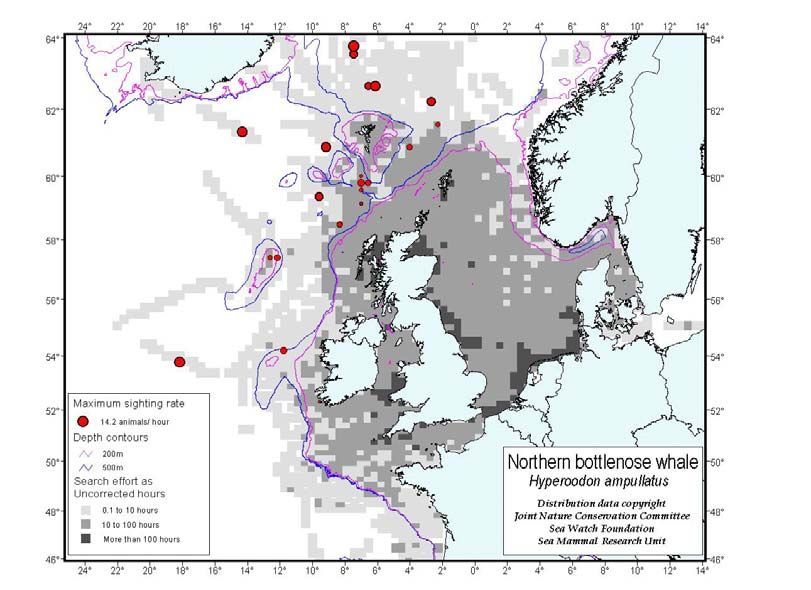
14 |                                                            ICES AGISC report 2005, 2nd edition

   to the typical dive profile characteristics, may accumulate over 300% nitrogen tissue
   supersaturation at the end of a typical dive sequence (Houser et al., 2001). This study, based
   on empirical observations of nitrogen tissue accumulation in bottlenose dolphins (Ridgway
   and Howard, 1979) and dive data from northern bottlenose whales Hyperoodon ampullatus
   (Hooker and Baird, 1999), suggested that beaked whales in particular may be more susceptible
   to acoustically mediated bubble formation than originally predicted by Crum and Mao (1996).

   Box 1 Decompression sickness and acoustically-mediated bubble formation

   Decompression sickness is the result of the supersaturation of body tissue with nitrogen and
   the subsequent release of bubbles of nitrogen gas. In human divers, decompression sickness is
   typically caused by rapid decompression following diving while using compressed air or
   repetitive, breath-hold dives. Unlike humans, the lungs of marine mammals collapse during a
   dive, limiting the nitrogen they carry to that which is absorbed into the blood stream within 60
   m to 100 m of the surface, although some pinnipeds dive on expiration and lung collapse
   occurs at much shallower depths (e.g. 25-50m in Weddell seals) (Falke et al., 1985). At
   greater depths, nitrogen is sequestered in non-exchanging airways. The amount of gas
   dissolved in specific tissues depends on dive depth, dive duration, descent and ascent rates,
   lipid content of the tissue, and surface intervals between successive dives. Progressive
   accumulation of nitrogen in tissues due to repetitive breath hold dives has been demonstrated
   empirically in bottlenose dolphins (Ridgway and Howard, 1979) and has been predicted to
   reach levels in excess of 300% supersaturation in northern bottlenose whales based on typical
   dive profiles (Houser et al., 2001).

   Although a number of anatomical, physiological, and behavioural adaptations that presumably
   guard against nitrogen bubble formation in marine mammals have been proposed (Ridgway
   1972, 1997; Ridgway and Howard, 1979, 1982; Falke et al., 1985; Kooyman and Ponganis,
   1998, Ponganis et al., 2003), it is possible that the gas emboli and associated lesions found in
   cetaceans in the Canary Islands and in the UK (Jepson et al., 2003; Fernandez et al., 2004, in
   press) could be caused by disruption of these evolutionary adaptations to deep diving.
   Anatomical and physiological adaptations to diving are unlikely to alter in the short course of
   acoustic exposure, but behavioural changes in response to sonar might. For example, in
   experiments northern right whales Eubalaena glacialis responded to novel acoustic stimuli by
   a combination of accelerated ascent rates and extended surface intervals at received sound
   levels as low as 133dB re 1µPa@1m (Nowacek et al., 2004). If beaked whales respond
   similarly they could experience excessive nitrogen tissue supersaturation driving potentially
   damaging bubble formation in tissues via a similar mechanism to the human diver that incurs
   DCS due to too rapid an ascent. Alternatively, physical mechanisms (e.g. rectified diffusion)
   exist for acoustically-mediated bubble formation in tissues already supersaturated with
   nitrogen (Crum and Mao, 1996; Houser et al. 2001).

   It is therefore theoretically possible that sonar transmissions (of low, mid or high frequency)
   could directly initiate or enhance bubble growth in tissues were sufficiently supersaturated
   with nitrogen and if the received sound pressure levels were of sufficient intensity. However,
   there is as yet no scientific evidence for any of the steps in these postulated chains of events.
   A (US) Marine Mammal Commission Workshop on beaked whales and anthropogenic noise
   considered it important to test the “bubble hypothesis”, and prioritised a programme of
   research that incorporates both acoustically mediated bubble formation and bubble formation
   via a DCS-like mechanism, and includes the use of controlled exposure experiments (Cox et
   al., in prep.).

   Even more recently, the first evidence of gas and fat emboli and acute and chronic gas bubble
   lesions has been reported in a number of cetacean species stranded in Europe. In the UK, ten
   stranded cetaceans comprising four Risso’s dolphins, four common dolphins, a Blainville’s
   beaked whale and a harbour porpoise had acute and chronic lesions in liver, kidney and
You can also read