Required Time Gap Between Mainshock and Aftershock for Dynamic Analysis of Structures

Required Time Gap Between Mainshock and
Aftershock for Dynamic Analysis of Structures
Roohollah M. Pirooz
 Kharazmi University
Soheila Habashi
 Kharazmi University
Ali Massumi (  ali.massumi@gmail.com )
 Kharazmi University https://orcid.org/0000-0003-4636-6553

Research Article

Keywords: time gap, seismic sequences, aftershock, zero acceleration interval, rest time

Posted Date: February 23rd, 2021

DOI: https://doi.org/10.21203/rs.3.rs-260285/v1

License:   This work is licensed under a Creative Commons Attribution 4.0 International License.
Read Full License

Version of Record: A version of this preprint was published at Bulletin of Earthquake Engineering on April
2nd, 2021. See the published version at https://doi.org/10.1007/s10518-021-01087-z.

Required time gap between mainshock and aftershock for dynamic analysis of
structures

Roohollah M. Pirooz, Master graduate of Structural Engineering, Kharazmi University
Postal address: Kharazmi University, No.43, Dr. Mofatteh Ave., Tehran, IRAN
ORCID iD: 0000-0003-0761-9351

Soheila Habashi, Master graduate of Structural Engineering, Kharazmi University
Postal address: Kharazmi University, No.43, Dr. Mofatteh Ave., Tehran, IRAN
ORCID iD: 0000-0002-1631-2979

Ali Massumi, Professor of Structural Engineering, Kharazmi University
Postal address: Kharazmi University, No.43, Dr. Mofatteh Ave., Tehran, IRAN
ORCID iD: 0000-0003-4636-6553

Corresponding author: Ali Massumi
Email address: massumi@khu.ac.ir
Telephone: +98 21 88830891

Abstract
 Despite the various studies carried out to evaluate the effects of seismic sequences on structures, the matter of the
time gap required to be considered between the mainshock and its corresponding aftershocks in dynamic analyses has
never been focused on directly. This subtle but in the meantime effective subject, influences on the amount of
accumulated damage caused by earthquake sequences. In the present study, 244 near fault ground motion components
from 122 earthquakes were applied to a wide variety of single degree of freedom systems having vibrating period of
0.05 to 7 seconds with linear and nonlinear behavior. Furthermore, 2 planar steel moment-resisting frames, having 3
and 12 stories, were subjected to a set of 30 ground motion components. The purpose of this investigation was to
estimate the required time for the structures to cease the free vibration at the end of the mainshock. The main purpose
is to generate an estimation that is function of structural system’s parameters and the strong motion duration. Excellent
correlations were obtained between the rest time and the following parameters: the combination of natural period of
single degree of freedom systems, as well as the strong motion duration of earthquake sequences. In consequence, a
formula is proposed which estimates the required optimized rest-time of a structure based on natural vibration period,
as well as the duration of strong motion. Additionally, results obtained from the dynamic analysis of the steel frames
validate the rest-time values achieved from the proposed formula.

Keywords: time gap; seismic sequences; aftershock; zero acceleration interval; rest time

1. Introduction
 The importance of aftershock effects on the responses of structures has been highlighted in several recent
studies. The effect of successive earthquakes is of high importance not only for more accurate evaluation of framed
structures and bridges (Xie et al. 2012) but also in maintaining the monuments and ancient structures (Papaloizou et
al. 2016). Examples of seismic events followed by aftershocks of comparable intensity have been observed in
various parts of the world, including in Italy (Friuli, 1976; Umbria-Marche, 1997), Greece (1986, 1988), Turkey
(1999) and Mexico (1993, 1994, 1995) (Li and Ellingwood 2007). A key feature in the application of seismic
sequences within the dynamic analysis of structures, is the time gap of a certain length inserted between the
mainshock and the corresponding aftershocks. This silent time interval with zero acceleration is actually applied in

dynamic analysis to ensure that the structure ceases the free vibration followed by the elimination of the seismic
excitation at the end of the ground motion’s time history (Goda 2012a, b).
 In the real situation, usually aftershocks do not occur right after the mainshock time history is terminated and
there is a time interval from a few minutes to several days between the mainshock and the subsequent aftershocks
(P. Gallagher et al. 1996). The aforementioned time gap is an opportunity for the structure to stop vibration due to
damping (Zhai et al. 2014). Amadio et al. (2003) considered a gap of about 40 seconds between successive events
for the structure to stop moving (Amadio et al. 2003). Hatzigeorgiou et al. (2009, 2010) applied a time gap between
the mainshock event and its following aftershocks which was equal to three times the single event duration
(Hatzigeorgiou and Beskos 2009; Hatzigeorgiou and Liolios 2010). In other studies by Hatzigeorgiou (2010), a time
gap of 100 s was applied between two consecutive seismic events (Hatzigeorgiou 2010a, b). Moustafa and Takewaki
(2011) applied the 40 seconds separating time interval between events (Moustafa and Takewaki 2011).
 Also, a silent time interval of 20 seconds was defined between the seismic sequence’s component (Ruiz-García
and Negrete-Manriquez 2011; Huang et al. 2012). Goda (2012) inserted 60 seconds of zeros, while in another study
by Goda (2015), 30 seconds of zeros was added between the repeated earthquake time histories to ensure that the
structural system returns to at-rest condition before the aftershock is applied (Goda 2012a, b, 2015). Zhai et al.
(2014) considered a time gap of 100 seconds and claimed that this time gap is sufficient for any civil structure to
stop vibrating due to damping (Zhai et al. 2013, 2014). Han et al. (2015) used different time gap for different
mainshock-aftershock sequences (Han et al. 2015). Mirtaheri et al. (2017) applied the aftershock sequences
immediately after the mainshock and claimed that the scenario could result in the most critical evaluation of their
structural models (Mirtaherf et al. 2017). Pu and Wu (2018) considered a time interval of 15 times the fundamental
period of structures employed for analysis (Pu and Wu 2018). Hosseini et al. (2019) considered 200 seconds of zero
acceleration time gap between selected sequences to ensure that the structure reaches the steady-state position
(Hosseini et al. 2019). Damage-based yield point spectra were developed for repeated earthquake ground motions by
analyzing single degree of freedom systems. In this work, a time gap of 100 seconds was considered between
mainshock-aftershock sequences (Zhang et al. 2020). Considering 20 seconds time gap, seismic performance of
buckling-restrained braced frames were evaluated under successive earthquakes (Hoveidae and Radpour 2020).
 This study is presented to investigate the required time for the structures to stop the free vibration with respect to
structural system’s properties and the ground motion’s features as the input parameters. Estimation of the minimum
required time gap for the dynamic analyses based on the above-mentioned parameters is worth regarding since a
wide variety of investigations conducted in earthquake engineering field to examine the effects of earthquake
sequences on structures, do confront it. On the other hand, the cost of analyses is of a great importance especially in
the repeated earthquake researches whereas the duration of seismic sequences is often long. Therefore, an optimized
estimation of the required time gap is needed.
 To this end, a formula is extracted using the curve fitting mathematical technique performed on the outputs of
linear and nonlinear analyses of single degree of freedom systems. The influence of strain hardening, damping and
ground motion scaling is taken into account in the proposed formulation. It is worth mentioning that results of two
steel moment-resisting frames with 3 and 12 number of stories were examined to assure the validity and accuracy of
the formulation.

2. Theoretical background
 As mentioned earlier, the rest time between the mainshock and the aftershock is defined as the time in which the
vibrating structure begins to enter the free vibration phase till the amplitude of vibration gradually is diminished and
gets close to the zero value at the end. It is illustrated in Fig. 1 to better understand the definition of rest time.
Therefore, the velocity response of the structure obtained from the equation of motion when solved for the free
vibration status after mainshock excitation, clarifies the rest time’s influential parameters.
The dynamic equilibrium equation of motion for a single degree of freedom system is given in Eq. (1) (Chopra 2006):

 ̈ + ̇ + = − ̈ (1)

where m is the mass of the system, c the viscous damping, k the stiffness, u the relative displacement, ̇ the relative
velocity, ̈ the relative acceleration and ̈ the ground motion acceleration.

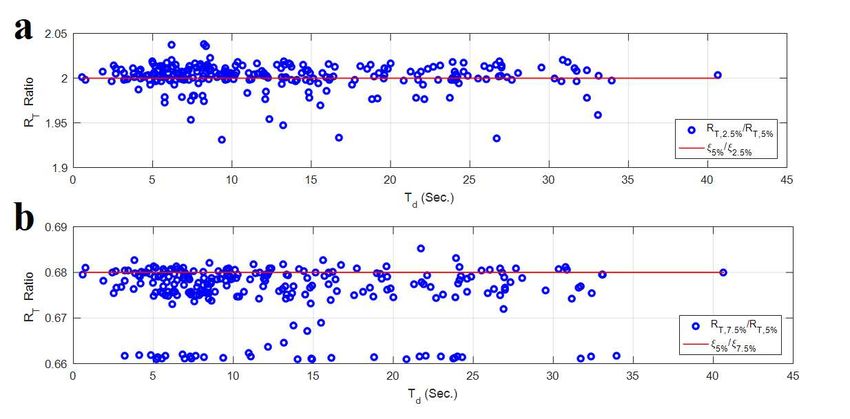
Fig. 1. An illustration of the rest time definition in a mainshock-aftershock earthquake record

If Eq. (1) is solved for a free vibrating system where the right term is set to zero, the general form of the velocity
response will be evaluated as depicted in Fig. 2.

 Fig. 2. General form of the velocity response of a SDOF system

 From Fig. 2, it is evident that the amplitude of vibrational response reduces with time and finally drops to the
value very close to zero. The time required for the velocity of the system to get close to zero, is a function of the
system’s damping ratio. The influence of damping on response of the system is also depicted in Fig. 3, in which the
velocity response of a SDOF system considering two different damping ratios is compared.

 Fig. 3. Effect of damping ratio on the amplitude of velocity response and the required time for the response to be
 fully damped

It is inferred that not only the amplitude of vibrational response is lessened as damping ratio is increased, but
also the required time for the system response to be fully damped and get close to zero value is shortened drastically
compared to the system with lower damping ratio ( = 2∙ 5%). A similar trend for the MDOF systems applies except
that mass (m), stiffness (k) and the damping coefficient (c) parameters are replaced by the mass, stiffness and
damping matrices and the acceleration, velocity and the displacement responses ( ̈ , ̇ , ) are replaced by their
corresponding vectors in Eq. (1) (Far 2017).

3. Description of structural models
3.1 Single degree of freedom models
22 elastoplastic single degree of freedom (SDOF) systems with the vibration period of T, ranging from 0.05 to 7
seconds are used in this study (Table. 1). The nonlinear behavior of SDOF systems is defined by a bilinear
elastoplastic force-displacement curve as shown in Fig. 4 (Samimifar et al. 2019). The equivalent bilinear force-
displacement curves were obtained through pushover analysis carried out on framed structures as was recommended
by Massumi and Monavari (2013) (Massumi and Monavari 2013). Strain-hardening ratio (h) or the ratio of post-
yielding stiffness to the initial stiffness of the model, is assumed to be 0%, 1%, 2% and 3%. The ratio of ultimate to
yield displacement (ductility) was set to 8 for all systems. Three values of 2.5%, 5% and 7.5% were also considered
for viscous damping ratio ( ) of SDOF systems. Response of the models to ground motion acceleration time
histories were computed using the Newmark = 1/4 numerical solution method of dynamic equation of motion
(Clough and Penzien 1995). It is worth mentioning that soil-structure interaction is not required to be modeled for
the assumed soil type (type II with shear velocity in range of 375-750 m/s) and conventional fixed base modeling is
reliable (Tabatabaiefar et al. 2012).

 Table 1. Fundamental period of vibration of single degree of freedom systems in seconds (T)
 0.05 0.10 0.15 0.20 0.25 0.50 0.75 1.00 1.25 1.50 1.75

 2.00 2.50 3.00 3.50 4.00 4.50 5.00 5.50 6.00 6.50 7.00

 Fig. 4. Nonlinear behavior model of an SDOF system

3.2 Multi degree of freedom models
 Two planar steel moment-resisting frames having 3 and 12 stories were modeled. The considered frames were
designed according to provisions of AISC 360-16 (2016) (2016) and ASCE 7-16 (2017) (2017).
 A more detailed description of the frame models is provided in Tables 2-3. The geometry and the elevation view
of the frame models are also illustrated in Fig. 5.
 The nonlinear behavior of columns and beams for dynamic analyses were assigned based on FEMA356
(Massumi and Mohammadi 2016) and is depicted in Fig. 6.

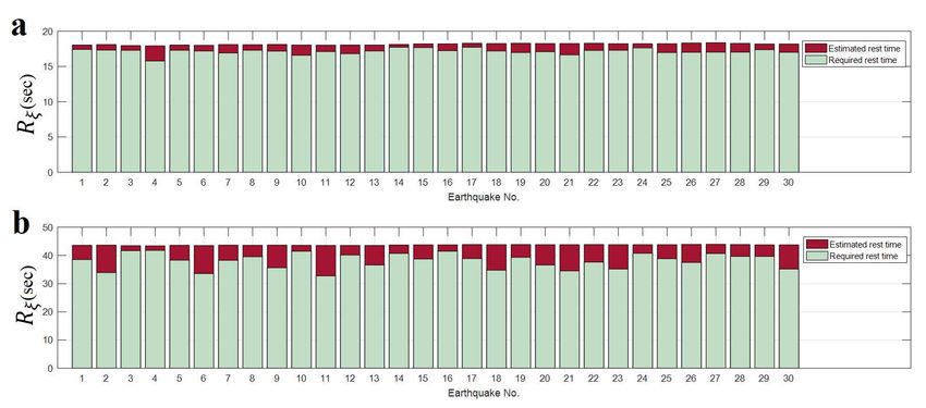
Table 2. Properties of the frame models
No. of Story No. of Bay Period of first
stories height (m) bays width (m) mode (sec.)

 3 3.2 4 4 0.81

 12 3.2 4 4 1.98

 Table 3. Steel sections of the frame models

Frame model Story Beams Columns

 1,2 IPE240 BOX200X15
 3 Story
 3 IPE200 BOX200X15

 1,2,3 IPE330 BOX400X20

 4,5,6 IPE330 BOX300X15

 7,8,9 IPE300 BOX250X15
 12 Story
 10 IPE270 BOX200X15

 11 IPE240 BOX200X15

 12 IPE200 BOX200X15

 Fig. 5. Elevation model of the steel frames

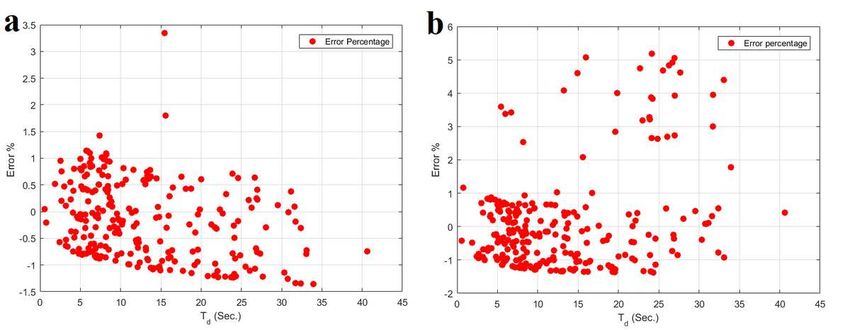
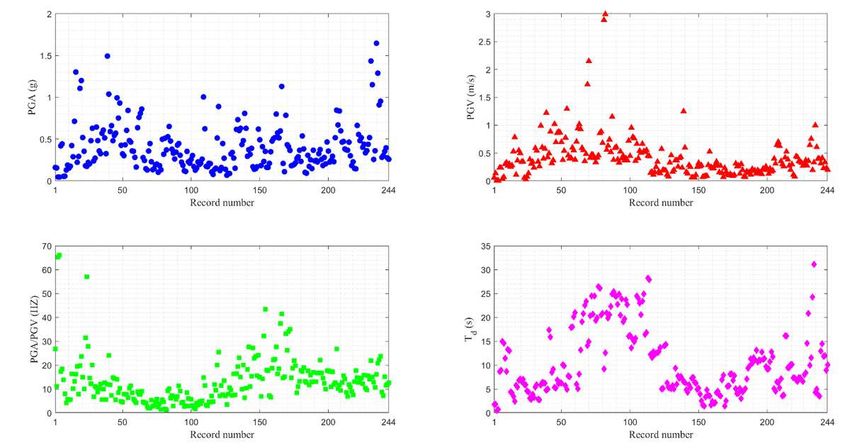
Fig. 6. Bilinear model of FEMA beam and column (D: end rotation or axial deformation, F: end moment or axial
 force, Ke: initial elastic slope, Kh: strain hardening slope, Kh/Ke = 0.02)

4. Description of selected earthquake ground motions
 In this study, a total of 244 earthquake acceleration time histories from 122 earthquake events (longitudinal (LN)
and transverse (TR) components) were employed for the dynamic analysis of the SDOF systems and a set of 30
acceleration time histories of the aforementioned ensemble were selected for the analysis of the steel frames.
During selection of records it is tried to include a wide variety of peak ground acceleration (PGA), peak ground
velocity (PGV), PGA/PGV ratio as a simple indicator of frequency content (Zhu et al. 1988) and strong motion
duration (Td) as the most important parameters on dynamic response of structures. Fig. 7 depicts the aforementioned
parameters of selected earthquake ground motions.

 Fig. 7. Descriptor parameters of selected records

 All the earthquake ground motions were downloaded from the Pacific Earthquake Engineering Research (PEER)
center database. Regarded earthquake records were selected based on the following criteria: (i) Magnitude ( ) of
the ground motions varies between 6 and 7.62; (ii) The shortest distance from the site to the rupture surface ( ) is
less than or equal to 10 kilometers (i.e., the selected records are near fault events); (iii) The average shear wave
velocity of top 30 m of the site ( 30 ) which corresponds to the soil type and site condition varies between 375 m/s
and 750 m/s conforming to site class C according to ASCE site classification.

The list of the considered earthquakes is shown in Table 4. Ground motions which were utilized for the analyses
of steel frames are highlighted and signed with star mark. The term T d in last column of the Table 4, indicates the
interval of 5-95% of squared ground acceleration cumulative integral which is identified as the most suitable
duration metric (Deierlein et al. 2012).

 Table 4. Earthquake ground motions employed for the analyses of SDOF systems
 Earthquak Rrup Vs30 PGA (g) PGA/PGV (Hz) Td (sec)
 No. Station Name Mw
 e Name (km) (m/s) LN TR LN TR LN TR
 Helena,
 1 Carroll College 6 2.86 593.35 0.16 0.16 26.73 11.40 1.74 1.82
 Montana-01
 Helena,
 2 Helena Fed Bldg 6 2.92 551.82 0.05 0.05 68.10 73.18 0.49 0.76
 Montana-02
 Anderson Dam
 3 Morgan Hill 6.19 3.26 488.77 0.42 0.29 16.22 10.23 4.385 4.205
 (Downstream)
 Coyote Lake Dam -
 4 Morgan Hill Southwest 6.19 0.53 561.43 0.71 1.3 13.17 16.26 3.425 2.41
 Abutment
 5 Morgan Hill Gilroy Array #6 6.19 9.87 663.31 0.22 0.29 19.28 7.80 5.79 5.415
 Big Bear Lake -
 6 Big Bear-01 6.46 8.3 430.36 0.48 0.54 14.84 14.28 8.52 9.18
 Civic Center
 7 Kobe, Japan Nishi-Akashi 6.9 7.08 609 0.48 0.46 10.29 11.26 7.72 7.56
 Duzce,
 8 Lamont 1058 7.14 0.21 529.18 0.11 0.08 7.35 4.83 12.28 11.61
 Turkey
 Duzce,
 9 Lamont 1059 7.14 4.17 551.3 0.14 0.15 12.16 9.40 12.81 12.24
 Turkey
 Duzce,
 10 Lamont 375 7.14 3.93 454.2 0.51 0.89 19.92 25.45 12.54 12.65
 Turkey
 Duzce,
 11 Lamont 531 7.14 8.03 638.39 0.12 0.16 6.93 11.45 12.87 13.65
 Turkey
 Chi-Chi,
 12 CHY074 6.2 6.2 553.43 0.32 0.34 9.53 7.27 5.235 5.06
 Taiwan-04
 13 Tottori, Japan SMN015 6.61 9.12 616.55 0.27 0.15 16.19 7.49 5.75 5.04

 14 Tottori, Japan SMNH01 6.61 5.86 446.34 0.62 0.73 16.52 19.36 9.39 6.01

 15 Tottori, Japan TTR009 6.61 8.83 420.2 0.6 0.63 22.98 15.09 7.77 7.25

 16 Bam, Iran Bam 6.6 1.7 487.4 0.81 0.63 6.36 10.36 6.565 6.33
 Parkfield-02, PARKFIELD -
 17 6 4.93 656.75 0.29 0.37 17.89 27.44 4.845 4.33
 CA DONNA LEE
 Parkfield-02, PARKFIELD -
 18 6 2.85 383.9 0.32 0.39 11.09 15.33 5.885 5.27
 CA EADES
 Parkfield-02, PARKFIELD -
 19 6 3.43 558.33 0.17 0.14 27.11 22.96 7.255 7.475
 CA GOLD HILL
 Parkfield-02, PARKFIELD -
 20 6 9.46 576.21 0.15 0.17 24.31 15.57 6.41 6.245
 CA JACK CANYON
 PARKFIELD -
 Parkfield-02,
 21 JOAQUIN 6 4.57 378.99 0.62 0.49 24.18 14.91 4.905 5.165
 CA
 CANYON
 PARKFIELD -
 Parkfield-02,
 22 MIDDLE 6 2.57 397.57 0.18 0.41 6.73 14.34 3.945 2.52
 CA
 MOUNTAIN
 PARKFIELD -
 Parkfield-02,
 23 STOCKDALE 6 4.83 393.56 0.23 0.35 31.77 42.95 1.67 1.465
 CA
 MTN
 Parkfield-02, Bear Valley Ranch,
 24 6 4.32 527.95 0.16 0.16 17.61 17.55 3.35 4.7875
 CA Parkfield, CA, USA
 25 Parkfield-02, Slack Canyon 6 2.99 648.09 0.21 0.35 7.24 6.54 3.675 3.56
 CA
 26 Parkfield-02, Parkfield - Cholame 6 4.08 522.74 0.48 0.51 18.92 22.43 1.645 2.43
 CA 2E
 27 Parkfield-02, Parkfield - Cholame 6 5.55 397.36 0.52 0.8 22.57 27.70 1.98 2.15
 CA 3E
 28 Parkfield-02, Parkfield - Cholame 6 4.23 410.4 0.58 0.51 16.47 18.41 4.285 4.525
 CA 4W
 29 Parkfield-02, Parkfield - Fault 6 4 541.73 0.6 1.13 37.59 41.42 3.725 3.57
 CA Zone 11

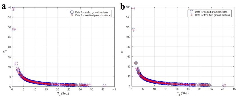
Table 4. Earthquake ground motions employed for the analyses of SDOF systems (continued)
 Earthquake Rrup Vs30 PGA (g) PGA/PGV (Hz) Td (sec)
No. Station Name Mw
 Name (km) (m/s) LN TR LN TR LN TR
 Parkfield-02, Parkfield - Gold Hill
30 6 6.3 450.61 0.21 0.11 14.72 15.15 6.94 7.905
 CA 3E
 Parkfield-02, Parkfield - Gold Hill
31 6 5.41 510.92 0.79 0.43 33.42 26.04 1.44 2.535
 CA 3W
 Parkfield-02, Parkfield - Gold Hill
32 6 8.27 421.2 0.41 0.36 34.10 34.61 5.55 5.675
 CA 4W
 Parkfield-02, Parkfield - Stone
33 6 5.8 566.33 0.18 0.19 14.62 18.99 8.115 8.195
 CA Corral 2E
 Parkfield-02, Parkfield - Stone
34 6 8.08 565.08 0.2 0.22 22.31 20.14 6.825 7.78
 CA Corral 3E
 Parkfield-02, Parkfield - Vineyard
35 6 2.96 381.27 0.27 0.29 8.50 11.00 5.1 4.07
 CA Cany 1E
 Parkfield-02, Parkfield - Vineyard
36 6 4.46 467.76 0.37 0.23 13.31 17.55 4.145 5.115
 CA Cany 2E
 Parkfield-02, Parkfield - Vineyard
37 6 3.52 438.74 0.54 0.38 17.36 18.81 3.03 4.425
 CA Cany 2W
 Parkfield-02, Parkfield - Vineyard
38 6 7.32 386.19 0.1 0.09 12.92 12.48 4.715 5.1
 CA Cany 4W
 Parkfield-02, PARKFIELD -
39 6 9.95 416.82 0.31 0.17 17.89 11.51 7.095 9.39
 CA UPSAR 02
 Parkfield-02, PARKFIELD -
40 6 9.95 440.59 0.25 0.15 15.57 13.22 9.8 11.32
 CA UPSAR 03
 Parkfield-02, PARKFIELD -
41 6 9.61 440.59 0.37 0.24 17.13 13.11 10.385 11.525
 CA UPSAR 05
 Parkfield-02, PARKFIELD -
42 6 9.61 440.59 0.25 0.23 13.24 16.98 11.175 13.15
 CA UPSAR 06
 Parkfield-02, PARKFIELD -
43 6 9.61 440.59 0.33 0.38 17.02 22.35 10.675 11.055
 CA UPSAR 07
 Parkfield-02, PARKFIELD -
44 6 9.41 440.59 0.26 0.18 16.86 14.25 10.99 12.74
 CA UPSAR 08
 Parkfield-02, PARKFIELD -
45 6 9.34 466.12 0.28 0.2 12.40 9.73 11.245 11.39
 CA UPSAR 09
 Parkfield-02, PARKFIELD -
46 6 9.41 466.12 0.47 0.36 17.86 17.98 9.725 9.155
 CA UPSAR 11
 Parkfield-02, PARKFIELD -
47 6 9.41 466.12 0.47 0.36 17.86 17.98 9.725 9.155
 CA UPSAR 11
 Parkfield-02, PARKFIELD -
48 6 9.47 466.12 0.23 0.25 17.69 11.09 9.255 10.74
 CA UPSAR 12
 Parkfield-02, PARKFIELD -
49 6 9.47 466.12 0.3 0.23 17.54 11.90 12.815 11.77
 CA UPSAR 13
 Duzce,
50 IRIGM 487 7.14 2.65 690 0.28 0.3 8.72 7.16 12.976 14.496
 Turkey
 Duzce,
51 IRIGM 498 7.14 3.58 425 0.35 0.4 14.99 11.69 11.868 12.004
 Turkey
 Parkfield-02,
52 Hog Canyon 6 5.28 376 0.28 0.26 12.13 12.72 8.93 10.08
 CA
 Irpinia, Italy-
53 Auletta 6.9 9.55 476.62 0.06 0.06 15.12 8.38 14.9698 14.5667
 01
 Irpinia, Italy-
54 Bagnoli Irpinio 6.9 8.18 649.67 0.13 0.19 4.22 5.69 11.4637 8.6681
 01
 Irpinia, Italy-
55 Calitri 6.2 8.83 455.93 0.15 0.18 5.37 5.79 13.2624 12.996
 02
 Kalamata,
56 Kalamata (bsmt) 6.2 6.45 382.21 0.24 0.27 6.85 11.03 3.8808 3.2352
 Greece-01
 Umbria
57 Nocera Umbra 6 8.92 428 0.47 0.38 15.48 14.20 3.575 3.715
 Marche, Italy
58 L'Aquila, GRAN SASSO 6.3 6.4 488 0.15 0.14 13.16 17.20 7.36 7.31
 Italy (Assergi)
59 L'Aquila, L'Aquila - V. Aterno 6.3 6.27 475 0.66 0.56 14.70 12.88 6.875 6.615
 Italy - Centro Valle
60 L'Aquila, L'Aquila - V. Aterno 6.3 6.81 685 0.48 0.52 13.34 14.70 7.355 7.39
 Italy -Colle Grilli
61 L'Aquila, L'Aquila - V. Aterno 6.3 6.55 552 0.4 0.44 12.17 15.78 6.92 6.59
 Italy -F. Aterno
62 L'Aquila, L'Aquila - Parking 6.3 5.38 717 0.34 0.36 10.49 9.54 7.995 8.39
 Italy

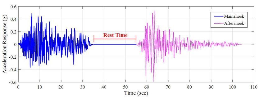
Table 4. Earthquake ground motions employed for the analyses of SDOF systems (continued)
 Earthquake Rrup Vs30 PGA (g) PGA/PGV (Hz) Td (sec)
No. Station Name Mw
 Name (km) (m/s) LN TR LN TR LN TR
 L'Aquila, GRAN SASSO
58 6.3 6.4 488 0.15 0.14 13.16 17.20 7.36 7.31
 Italy (Assergi)
 L'Aquila, L'Aquila - V. Aterno
59 6.3 6.27 475 0.66 0.56 14.70 12.88 6.875 6.615
 Italy - Centro Valle
 L'Aquila, L'Aquila - V. Aterno
60 6.3 6.81 685 0.48 0.52 13.34 14.70 7.355 7.39
 Italy -Colle Grilli
 L'Aquila, L'Aquila - V. Aterno
61 6.3 6.55 552 0.4 0.44 12.17 15.78 6.92 6.59
 Italy -F. Aterno
 L'Aquila,
62 L'Aquila - Parking 6.3 5.38 717 0.34 0.36 10.49 9.54 7.995 8.39
 Italy
 Nahanni,
63 Site 1 6.76 9.6 605.04 1.11 1.2 19.92 23.65 6.835 7.085
 Canada
 Nahanni,
64 Site 2 6.76 4.93 605.04 0.52 0.36 14.99 10.19 6.5975 7.04
 Canada
 Nahanni,
65 Site 3 6.76 5.32 605.04 0.18 0.17 31.13 55.75 5.9725 5.92
 Canada
 Cape
66 Cape Mendocino 7.01 6.96 567.78 1.49 1.04 11.95 24.05 4.74 4.96
 Mendocino
 Cape
67 Petrolia 7.01 8.18 422.17 0.59 0.66 11.73 7.31 17.34 15.88
 Mendocino
 Jensen Filter Plant
68 Northridge-01 6.69 5.43 525.79 0.57 0.99 5.48 13.96 5.335 5.215
 Generator Building
 LA - Sepulveda VA
69 Northridge-01 6.69 8.44 380.06 0.75 0.93 8.55 10.33 6.87 6.135
 Hospital
70 Northridge-01 LA Dam 6.69 5.92 628.99 0.43 0.32 4.87 4.50 6.395 6.2
 * Pacoima Kagel
71 Northridge-01 6.69 7.26 508.08 0.3 0.43 7.86 7.80 10.1 9.84
 Canyon
 Sylmar - Olive View
72* Northridge-01 6.69 5.3 440.54 0.6 0.84 7.59 6.37 5.74 4.94
 Med FF
 Chi-Chi,
73 TCU078 6.2 7.62 443.04 0.45 0.27 7.69 13.43 5.02 5.16
 Taiwan-03
 Chi-Chi,
74 TCU084 6.2 9.32 665.2 0.14 0.07 7.22 3.70 14.075 14.305
 Taiwan-03
 Chi-Chi,
75 TCU089 6.2 9.81 671.52 0.09 0.09 7.92 10.80 6.29 5.38
 Taiwan-03
 San Simeon, Templeton - 1-story
76 6.5 6.22 410.66 0.44 0.48 10.07 19.91 7.62 7.155
 CA Hospital
77* Niigata, Japan NIG028 6.63 9.79 430.71 0.52 0.85 12.75 26.88 5.09 4.515

78 Niigata, Japan NIGH01 6.63 9.46 480.4 0.67 0.84 10.19 11.77 6.515 6.325
 *
79 Niigata, Japan NIGH11 6.63 8.93 375 0.6 0.46 9.38 12.69 5.255 7.14
 Montenegro, Bar-Skupstina
80 7.1 6.98 462.23 0.37 0.37 8.64 6.92 16.15 16.11
 Yugo. Opstine
 Montenegro, Petrovac - Hotel
81 7.1 8.01 543.26 0.46 0.3 11.78 10.73 9.46 9.51
 Yugo. Olivia
 Montenegro, Ulcinj - Hotel
82 7.1 4.35 410.35 0.18 0.23 8.83 7.58 10.16 10.16
 Yugo. Albatros
83 Iwate IWTH24 6.9 5.18 486.41 0.44 0.52 15.68 14.24 14.58 20.83
 *
84 Iwate IWTH25 6.9 4.8 506.44 1.43 1.15 21.84 14.93 10 11.55
 Mizusawaku Interior
85 Iwate 6.9 7.85 413.04 0.26 0.36 13.05 10.65 24.24 31.09
 O ganecho
 N. Palm
86* Cabazon 6.06 7.92 376.91 0.22 0.2 27.76 14.28 4.615 4.35
 Springs
 N. Palm Whitewater Trout
87 6.06 6.04 425.02 0.48 0.63 12.25 20.10 3.08 2.83
 Springs Farm
 *
88 Loma Prieta Corralitos 6.93 3.85 462.24 0.64 0.48 10.67 8.65 5.415 5.895
 * Gilroy - Gavilan
89 Loma Prieta 6.93 9.96 729.65 0.36 0.33 10.19 12.25 2.845 2.73
 Coll.
 *
90 Loma Prieta LGPC 6.93 3.88 594.83 0.57 0.61 5.64 9.94 5.82 6.41
 Saratoga - Aloha
91 Loma Prieta 6.93 8.5 380.89 0.51 0.33 12.51 5.62 6.3 6.2
 Ave

Table 4. Earthquake ground motions employed for the analyses of SDOF systems (continued)
 Earthquake Rrup Vs30 PGA (g) PGA/PGV (Hz) Td (sec)
No. Station Name Mw
 Name (km) (m/s) LN TR LN TR LN TR
 Chi-Chi,
92 CHY006 7.62 9.76 438.19 0.36 0.36 8.50 5.92 17.884 18.04
 Taiwan
 * Chi-Chi,
93 CHY024 7.62 9.62 427.73 0.28 0.17 5.00 4.38 20.115 20.99
 Taiwan
 Chi-Chi,
94* CHY028 7.62 3.12 542.61 0.64 0.76 8.92 7.90 6.015 5.055
 Taiwan
 Chi-Chi,
95* CHY080 7.62 2.69 496.21 0.81 0.86 7.81 9.10 8.125 13.185
 Taiwan
 Chi-Chi,
96* TCU049 7.62 3.76 487.27 0.28 0.24 4.64 4.25 19.125 20.805
 Taiwan
 Chi-Chi,
97* TCU050 7.62 9.49 542.41 0.15 0.13 4.16 2.65 22.53 23.34
 Taiwan
 Chi-Chi,
98* TCU052 7.62 0.66 579.1 0.36 0.45 2.04 2.05 14.12 14.91
 Taiwan
 Chi-Chi,
99* TCU053 7.62 5.95 454.55 0.23 0.13 5.43 2.70 20.355 24.485
 Taiwan
 Chi-Chi,
100* TCU054 7.62 5.28 460.69 0.15 0.19 3.15 4.52 20.685 24.485
 Taiwan
 Chi-Chi,
101* TCU060 7.62 8.51 375.42 0.2 0.1 5.81 2.33 19.395 19.895
 Taiwan
 Chi-Chi,
102* TCU063 7.62 9.78 476.14 0.18 0.13 3.86 1.49 26.46 26.14
 Taiwan
 Chi-Chi,
103 TCU068 7.62 0.32 487.34 0.51 0.37 1.73 1.21 9.19 12.58
 Taiwan
 Chi-Chi,
104 TCU071 7.62 5.8 624.85 0.53 0.65 9.33 10.09 20.945 19.86
 Taiwan
 Chi-Chi,
105 TCU072 7.62 7.08 468.14 0.48 0.38 6.34 7.18 20.565 22.3
 Taiwan
 Chi-Chi,
106 TCU075 7.62 0.89 573.02 0.33 0.26 2.81 6.78 24.94 25.39
 Taiwan
 Chi-Chi,
107 TCU076 7.62 2.74 614.98 0.34 0.43 5.65 6.91 24.515 24.445
 Taiwan
 Chi-Chi,
108 TCU078 7.62 8.2 443.04 0.45 0.31 11.46 9.27 22.73 24.855
 Taiwan
 Chi-Chi,
109 TCU082 7.62 5.16 472.81 0.23 0.19 4.28 4.60 20.44 23.86
 Taiwan
 Chi-Chi,
110 TCU087 7.62 6.98 538.69 0.12 0.11 2.61 2.94 19.12 19.69
 Taiwan
 Chi-Chi,
111 TCU089 7.62 9 671.52 0.35 0.23 8.50 6.10 23.675 22.665
 Taiwan
 Chi-Chi,
112 TCU101 7.62 2.11 389.41 0.21 0.26 2.86 5.70 16.045 16.22
 Taiwan
 Chi-Chi,
113 TCU102 7.62 1.49 714.27 0.3 0.17 3.08 2.12 13.615 15.43
 Taiwan
 Chi-Chi,
114 TCU103 7.62 6.08 494.1 0.13 0.15 1.67 4.08 14.945 15.63
 Taiwan
 Chi-Chi,
115 TCU120 7.62 7.4 459.34 0.23 0.2 3.39 4.84 24.495 24.02
 Taiwan
 Chi-Chi,
116 TCU122 7.62 9.34 475.46 0.21 0.26 3.82 5.07 23 20.58
 Taiwan
 Chi-Chi,
117 TCU129 7.62 1.83 511.18 1 0.62 14.73 11.43 23.405 24.935
 Taiwan
 Chi-Chi,
118 TCU136 7.62 8.27 462.1 0.17 0.17 3.21 3.01 16.432 16.816
 Taiwan
 Chi-Chi,
119 TCU138 7.62 9.78 652.85 0.21 0.21 4.57 4.64 28.24 27.928
 Taiwan
 Christchurch, Heathcote Valley
120 6.2 3.36 422 1.65 1.29 16.23 20.82 4.335 4.96
 New Zealand Primary School
 Christchurch,
121 LPCC 6.2 6.12 649.67 0.91 0.95 22.25 23.64 3.82 3.505
 New Zealand
 Mammoth
122* Convict Creek 6.06 6.63 382.12 0.42 0.44 17.34 18.34 8.69 8.925
 Lakes-01

5. Analysis procedure and results
5.1 Response of the SDOF systems
 In this section, the implemented methodology and related outcomes are discussed. At first, all of the 244
acceleration time histories were scaled record by record so as their maximum acceleration was equal to 1.0g, that is,
each record was divided by its PGA. The 5-95% significant duration ( ) of each time history along with 2.0
seconds of the time history before the was considered. Then, a time interval of sufficient length with zero
acceleration was inserted at the end of each time history.
 It is worth noting that the aforementioned time interval was embedded at the end of the time histories in order to
monitor the velocity response of the systems during the free vibration. In fact, when successive ground motions (i.e.,
mainshock-aftershock seismic sequences) happen, there is often a time gap between the mainshock and the
subsequent aftershocks which may be lasting from a few minutes to even a several days. Since the cost of analysis is
of a great importance specially in the nonlinear time history analysis, an optimized estimation of the required time
gap (i.e., a specified interval of the time with zero acceleration during which the structural model’s velocity response
approaches a value close to zero or the time needed for the structure to stop free vibration.) is necessary to be
determined. For this purpose, a sufficient time gap was applied at the end of the acceleration time histories to make
sure that the velocity response of the SDOF systems reaches a value very close to zero ( ). In this study, it is
assumed that if the free vibration velocity response of the system becomes less than or equal to the 0.1% of the
maximum free vibration velocity response ( . ) of the system and it does not increase anymore, the structural
model stops free vibration (Eq. (2)). In this study, the upper limit in Eq. (2), was set to 0.1% of the . .

 ≤ (2)

 For this purpose, the time required for the free vibrations velocity of the system to reach was extracted
using trial and error procedure. Thus, zero acceleration interval of 50 seconds was initially considered. If the
assumed interval is not enough for approaching zero velocity, the interval will be increased to 100 seconds. This
would be applied iteratively until the required rest time is extracted with acceptable accuracy.
 After performing the dynamic time history analyses on the SDOF systems, the velocity responses were processed
and the required time for each SDOF system to stop free vibration (rest time) was extracted according to the method
discussed above. It should be noted that the same procedure was done for the MDOF systems supposed that the
velocity responses of the roof level be used. Rest time of the SDOF systems were plotted against the 5-95%
significant duration of the ground motions. Fig. 8 shows the resulted plots for the SDOF systems with fundamental
period (T) of 1.0 s and 4.0 s.

Fig. 8. Evaluated rest time of the SDOF systems versus strong motion duration: (a) SDOF system with fundamental
 period (T) of 1.0 sec., (b) SDOF system with T = 4.0 sec.

 In another try, rest time of the SDOF systems were normalized by 5-95% significant duration of the
corresponding record and a comparison was carried out between the normalized rest time data series (RT) and the
significant duration ( ) of the earthquake records to observe the changing trend. The related plots for the SDOF
systems with T = 1.0 s and T = 4.0 s are illustrated in Fig. 9 (a) and Fig. 9 (b) respectively.

Fig. 9. Normalized rest time (RT) of the SDOF systems versus strong motion duration: (a) SDOF system with T =
 1.0 sec., (b) SDOF system with T = 4.0 sec.

 According to the Fig. 9 (a) and Fig. 9 (b), it is obvious that the normalized rest time (RT) of an SDOF system is
strongly correlated with the strong motion duration of the applied ground motions and as the strong motion duration
increases, the normalized rest time decreases in a regular nonlinear trend, but results of the mere rest time (non-
normalized data), versus strong motion duration (see Fig. 8) looks less encouraging. It seems that the rest time is not
straightly related to the strong motion duration as it is depicted in Fig. 8, but by normalizing the evaluated rest time
with respect to the corresponding strong motion duration of each earthquake record, the negative nonlinear
correlation of the normalized rest time and the strong motion duration data series becomes evident.
The strong emerged relationship between the parameters RT and Td for the SDOF systems with fundamental period
(T) ranging from 0.05 to 7.0 s, leads to curve fitting of data series. This way, evaluated normalized rest time of the
SDOF systems (RT) was expressed as the function of strong motion duration (T d) and the fundamental vibration
period (T) of the SDOF systems. Details on the computational tool and the mathematical operations on the data
series is explained in the following section.

5.2 Proposed formulation and related mathematical computation
 As mentioned in the earlier section, for each of the SDOF systems with a given vibrational period (T), the
normalized rest time (RT) data series were plotted against the strong motion duration (T d) for all the 244 applied
earthquake components. Therefore, 22 (number of SDOF systems) graphs illustrating RT against Td for each SDOF
system such as the one in Fig. 9(a) were extracted. The observations showed that the normalized rest time data series
(RT) and the strong motion duration data series (T d) are strongly correlated in a nonlinear reverse order in all the
cases. Accordingly, regression analyses were performed on each of the outcome graphs so as to find the curve that
best fits to the observed data points. The curve fitting technique utilizing the nonlinear least squares method was
employed in this study to extract the aforementioned curves or functions (Hansen et al. 2013). The general form of
the assumed function for the fitted curve is written as the form of Eq. (3):

 = + (3)

where x indicates the strong motion duration of each earthquake (T d), y is the estimated normalized rest time (RT,
estimate) with respect to T d data and a, b and c are the coefficient of the equation which are obtained by fitting the
assumed function to the observed data points. Thus the Eq. (3) is converted to the following form of Eq. (4):

 . = ( ) + (4)

 By fitting the curve of the assumed form to each of the 22 observed datasets for SDOF systems, the coefficients
a, b and c were determined. Examples of the fitted curve versus the observed data (from the time history analyses)
are shown in Fig. 10. It can be seen that the fitted curve is matched well by the observed data points. Results for the
other examined SDOF systems are similar.

Fig. 10. Curves fitted to the normalized rest time (RT) plotted versus the strong motion duration (T d): (a) for T = 1.0
 s, (b) for T = 4.0 s

 In order to evaluate the goodness of the fit, the percentage of error, defined in Eq. (5) is calculated:

 % = (( . − )/ ) × 100 (5)

where . represents the normalized rest time estimated by the fitted function and is the normalized
required rest time obtained from the SDOF analysis.

Fig. 11. The percentage of difference between the collected rest time and the determined rest time obtained from the
 fitted curve’s formula: (a) for T = 1.0 s, (b) for T = 4.0 s

 As shown in Fig. 11, the absolute value of the error percentage is no more than the 5% meaning that the assumed
curve is fitted well enough. Results of the remaining SDOF models are also analogous. Implementation of the curve
fitting process resulted in the constant coefficients a, b and c for each of the SDOF systems.
 Tracking the changes of the ‘a’ coefficient with regard to the changes of the fundamental vibration period of the
SDOF systems, a linear relation between the two parameters was figured out as is illustrated in Fig. 12(a). But
variation of the two other coefficients ‘b’ and ‘c’ over the changes of the vibrational period are nearly around zero
value as shown in Fig. 12(b) and Fig. 12(c) respectively. Hence, conservatively the upper limit of data was
considered for these two coefficients.

Fig. 12. Curves fitted to the coefficients of the Eq. (3) plotted along with the obtained coefficients as a function of
fundamental vibration period of SDOF systems: (a) for “a” coefficient, (b) for “b” coefficient, (c) for “c” coefficient

 The coefficients for the SDOF systems with the damping ratio ( ) of 5% and the hardening slope (h) equal to
3% can be expressed as Eq. (6), Eq. (7) and Eq. (8):

 ( ) = 21∙ 8559( ) + 0∙ 0258 (6)

 = −0∙ 9982 (7)

 = 0∙ 0214 (8)

in which, T represents the fundamental vibration period of the SDOF system and ( ) indicates the ‘a’ coefficient
as a function of the vibration period for the corresponding SDOF system with a specified T. Now, Eq. (4) along with
the obtained Eq. (6,7,8) can come together and be written as Eq. (9):

 . = (21∙ 8559 + 0∙ 0258)( )−0.9982 + 0∙ 0214 (9)

 The proposed equation (Eq. (9)), estimates the optimum normalized rest time of a structure as a function of the
vibration period (T) and the strong motion duration of the applied earthquake component (T d). The Estimated
normalized rest time ( . ), should finally be multiplied by T d to obtain the required rest time for the structure
(R) as follows:

 = [ (21∙ 8559 + 0∙ 0258)( )−0∙9982 + 0∙ 0214] (10)

 The proposed formulation estimates the minimum required rest time of a nonlinear system with = 5% and
hardening slope (h) of 3% which is subjected to the scaled ground motions. In order to develop the use of the
proposed formulation in a more general term, influences of the linearity of modeling, ground motion scaling,
different hardening slope and the effect of various damping ratios are investigated and the results are explained
comprehensively in the following sections.

5.3 Linearity versus nonlinearity
 In addition to the nonlinear SDOF systems, a group of linear SDOF systems having only the linear part of the
bilinear behavior and the same vibrational periods, were also modeled and analyzed. Results of the linear models as
well as the nonlinear systems, under scaled ground motions and for the damping ratio of 5% is illustrated in Fig.
13(a) and Fig. 13(b) for instances.
 It is inferred that no matter systems behave linearly or nonlinearly, the required rest time is identical. Therefore,
the proposed formulation for the rest time calculation (Eq. (10)), is appropriate for both the linear systems as well as
the nonlinear systems.

Fig. 13. Normalized rest time (RT) plotted against strong motion duration (T d) for the collected data of a linear
SDOF system as well as a nonlinear SDOF system: (a) for an SDOF with T = 0.05 s, (b) for an SDOF with T = 7.0 s

5.4 Influence of ground motion scaling
 Ground motion components were once applied as the free field records and in another try, they were scaled to a
common value such that their peak ground acceleration (PGA) be equal to 1.0 time the ground acceleration (g or
9.806 m/s2) to make a basis for comparison. Rest time results in both the scaled and the free field conditions were
extracted separately. A comparison between the normalized rest time of the nonlinear SDOF systems while
subjected to the scaled ground motions and the same systems in case they were analyzed under the free field ground
motions was conducted.
 As is shown in Fig. 14, the effect of ground motion scaling can be ignored since the rest time obtained using
scaled ground motion is same as the one yielded by the free field earthquake record. It should be noted that the
results shown in Fig. 13 (for nonlinear SDOF systems with 3% hardening slope and the 5% damping ratio) were
confirmed for the remaining SDOF systems.

Fig. 14. Normalized rest time (RT) plotted against strong motion duration (T d) While using scaled ground motions as
 well as free field ground motions: (a) for T = 1.0 s, (b) for T = 4.0 s

5.5 Influence of hardening slope
 Impacts of defining different hardening slopes for nonlinear behavior of systems on the required rest time has
also been investigated. Observing Fig. 15, it is readily figured out that the rest time outputs for the assumed
hardening slope of 3% conforms to the results for the 1% hardening slope. Therefore, different assumptions for the
hardening slope (h) parameter in the nonlinear description of models, are not going to influence on the required rest
time of the system.

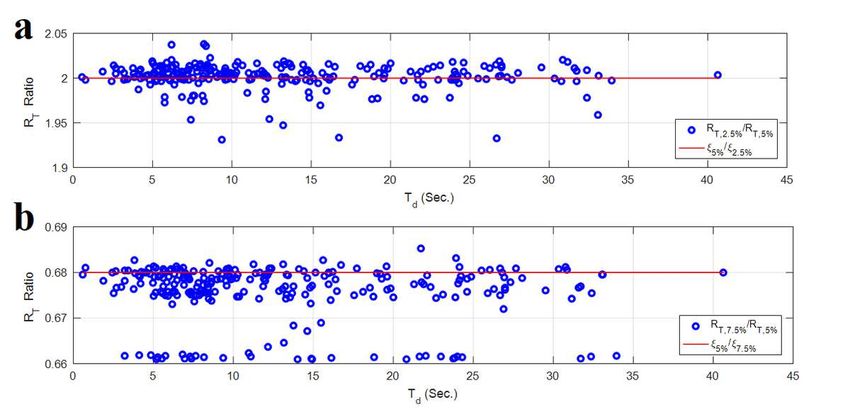
Fig. 15. Normalized rest time (RT) plotted against the strong motion duration (T d) for different hardening slopes of
 nonlinear behavior: (a) for T = 1.0 s, (b) for T = 4.0 s

5.6 Influence of damping ratio
 A key factor that the required rest time of a system is influenced by, is damping ratio since this parameter is
directly concerned with the energy dissipation of a system. It is expected as the damping ratio increases, the free
vibration of structural system after mainshock be damped more rapidly.
Hence, the effect of above-mentioned parameter was examined for three groups of SDOF systems having damping
ratio of 2.5%, 5% and 7.5% respectively. Rest time results for the three values of damping ratio are presented in Fig.
16. As the damping ratio decreases, the rest time curve moves upward meaning that the rest time demand rises up.
Therefore, required rest time of the system is related to the damping ratio conversely.

 Fig. 16. Normalized rest time (RT) plotted against the strong motion duration (T d) data series using different
 damping ratios: (a) for T = 1.0 s, (b) for T = 4.0 s

 To deal with the damping ratio effect on the rest time response of the system, ratio of normalized rest time of the
SDOF systems while = 2.5% ( .2.5% ) to the normalized rest time of the systems while = 5% ( .5% ), was
calculated and compared with 5% / 2.5% ratio (which is equal to 0.05/0.025) in Fig. 16 for a SDOF system with T =
1.0 s as an example. It is shown that .2.5% / .5% values are almost entirely close to the continuous line of data
representing the 5% / 2.5% value. For instance, in Fig. 17(a), RT ratios vary between 1.95 and 2.05 mostly which
means that the RT ratios approach the value of 5% / 2.5% or 2.0.

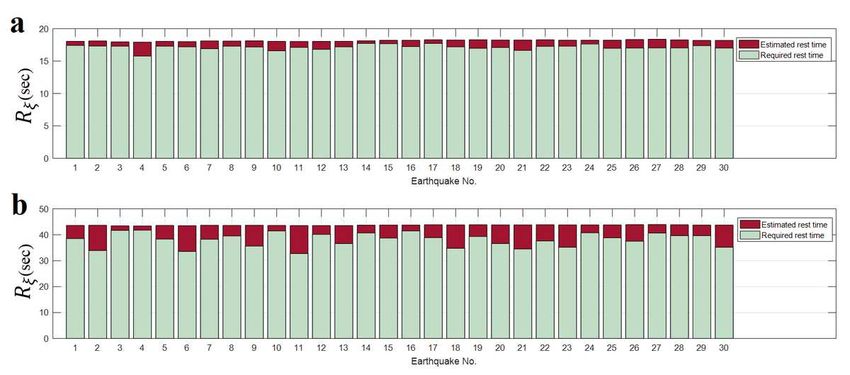
Fig. 17. The ratio of normalized rest time (RT) versus strong motion duration (T d) for a SDOF having two different
 damping ratios with respect to the 5% damping ratio: (a) for = 2.5%, (b) for = 7.5%

 It was demonstrated that for all other examined SDOF systems, the following relation in Eq. (11) is confirmed:

 . 5% (11)
 ≅
 .5% 

in which . represents the normalized rest time for a damping ratio of interest ( ), .5% is the normalized rest
time for = 5% and the parameters 5% and are damping ratio of 5% and target damping, respectively.
The proposed formulation was extracted for the commonly used damping ratio of 5%. In order to generalize the
application for any desired damping ratio and take the damping effect into account, Eq. (9), Eq. (10) and Eq. (11)
were assembled and resulted in Eq. (12):

 5% (12)
 = ( )[ (21∙ 8559 + 0∙ 0258)( )−0∙ 9982 + 0∙ 0214 ]
 
where is the required rest time of the system for the arbitrary damping ratio of . Therefore, Eq. (10) was
modified so that it could deal with the damping ratio effect. Finally, the proposed formulation in Eq. (12) estimates
the required rest time of a system as a function of input parameters or fundamental vibration period of structure, 
or damping ratio of structure and or strong motion duration.

5.7 Response of MDOF steel frames and validation
 Promising results of the SDOF systems encouraged the authors to evaluate the proposed formulation for the
MDOF systems. For this purpose, two steel moment resisting frames with 3 and 12 number of stories representatives
of low-rise and mid-rise frames respectively were modeled. Design details and other considerations of the structural
models were explained previously in section 3.
 Since the ground motions should be commonly scaled in nonlinear analyses, a set of 30 scaled ground motions
were applied to each of the steel frames. The ground motions were multiplied by a factor to match the average
response spectrum for the 10% probability of exceedance in 50 years (10/50) hazard level. Also, a damping ratio of
5% was set for nonlinear dynamic analysis of MDOF systems.
 Required rest time for each of the frames were calculated based on the procedure discussed earlier in section 4.1
and were compared to the estimated rest time determined using the proposed formulation in this paper (Eq. (12)).
Fig. 18 illustrates the required rest times for each frame versus the estimated rest times extracted from the proposed
formulation.

Fig. 18. Required rest time obtained from the analysis versus the estimated rest time using the proposed formulation:
 (a) for the 3-story steel frame, (b) for the 12-story steel frame

 It is observed that the proposed formula gives a good estimation for the required rest time and the differences
between the estimated values and the required values are almost small especially for the low-rise frame. In fact, the
proposed formula estimates the rest time conservatively.
 The agreement between the rest time data obtained from the nonlinear analyses of frames and the rest time data
estimated using the proposed formula was also investigated and as the results in Fig. 19 reveal, there is a satisfactory
agreement between them. Therefore, the proposed formulation gives an appropriate estimation both for SDOF
systems as well as MDOF systems.

 Fig. 19. Normalized rest time (RT) plotted against the strong motion duration (T d) data series using different
 damping ratios: (a) for T = 1.0 s, (b) for T = 4.0 s

6. Discussion
6.1 Detailed examination of required rest time against system period and strong motion duration
 To better understand the influence of strong motion duration on the required rest time of structures with different
vibration periods, maximum and minimum rest time for each of the vibration periods considering different strong
motions (Td), were calculated. Rest time results as a function of vibration periods (T) is displayed in Fig. 20 for the
maximum and minimum values. From Fig. 20, first of all it is readily observed that the rest time is totally increased
as the system’s vibration period is increased.
 Fig. 20 also points out to the difference between maximum and minimum required rest time in short periods
compared to the long periods.

Fig. 20. Maximum and minimum rest time plotted against the vibration period

It is shown that the difference between the maximum and minimum rest times is more apparent in long periods. In
fact, for systems with vibration period of less than 1.0 s, the differences are almost negligible. Since the maximum
and minimum rest times were calculated considering different strong motion durations, it is inferred that the
influence of strong motion duration (Td) on the required rest time of a system with vibrating period of less than 1.0 s
(short periods), is slight and can be ignored but as the period increases (over 1.0 s), the impact of strong motion
duration appears to be important. For example, for the vibration period of a system being equal to 7.0 s, the
difference between the maximum rest time and minimum rest time (which were calculated for two different values
of Td), is around 20 s but the difference for a system with vibrating period of 1.0 s is close to zero value. Therefore,
rest time of a system depends strongly on the strong motion duration as well as the vibrating period of system
specially for systems with long periods. Fig. 20, also gives a general insight to the required rest time for an
applicable range of vibrating periods. It is worth mentioning that the proposed formula conservatively estimates the
upper limit value for the rest time.

6.2 Scope of the study
 It is valuable to clearly explain the limitations and scope of this study. This would greatly help to better
understand the main goal of this work. Also, considering these limitations, the future studies to strengthen the
findings of this paper can be determined.
 As stated earlier, the prime objective of this work is to develop a framework to include the required rest time
between mainshock-aftershock sequence in dynamic analysis of structures. The results showed that the time gap
between mainshock-aftershock sequence can be efficiently estimated using system properties and strong motion
duration of earthquakes. Although these results demonstrate the validity of this claim, but it should be expected that
developed formula can evolve if the inputs of described analysis procedure change.
 The first important parameter is the selected earthquake records. In this work, relatively a large number of
records have been selected, but it cannot be argued that they can represent all seismic characteristic of earthquake
ground motion. For example, selected events are all near field records which belong to site class C according to
ASCE site classification. One may expect including mid and far fault events recorded on other type of sites would
affect final results.
 Second, the effect of stiffness degradation and the strength deterioration was not considered for the SDOF and
MDOF models of the structures. This phenomenon may change the required rest time for a structure after the
mainshock.
 Finally, the evaluated formula by dynamic analysis of SDOF systems has directly applied to MDOF structures. It
is worthy to consider structures with different height and lateral resisting frame to improve the formula for real
world applications.

These are the main limitations of this study which determine the scope of presented work. These limitations can
be the subject of future studies to finally develop a comprehensive method for estimating required rest time for
different structures located on different seismogenetically active regions.

7. Conclusions
 In this paper, a novel formulation is introduced to estimate the required rest time between mainshock and
aftershock in nonlinear dynamic analysis of structures. The proposed formula evaluates the required rest time with
respect to structural system’s properties (vibrational period) and the ground motion’s feature (strong motion
duration). A set of 244 ground motion components for the nonlinear dynamic analyses of SDOF systems were
considered in the current study. 30 earthquake records were also used for the analyses of steel frames and validation
of the obtained results. In order to generalize the proposed formulation, influences of different parameters such as
structural behavior (linearity or nonlinearity), ground motion scaling, hardening slope in bilinear behavior and
damping ratio were investigated and taken into account. Finally, the proposed formulation was validated for low and
mid-rise MDOF steel frames. Important conclusions accomplished in this study are outlined:
 Required rest time is strongly correlated with strong motion duration and vibration period of the structure. Ther
 efore, the output of the proposed formulation is the required rest time as a function of these two parameters.
 Rest time results for linear models was analogous to the rest time results of the nonlinear models. Hence, the req
 uired rest time of a system does not depend on the level of nonlinearity that a system experiences.
 Whether using the scaled earthquake ground motions or the free field ones, the required rest time is identical. T
 herefore, the effect of ground motion scaling on the required rest time is ignored.
 Application of different hardening slopes in the bilinear modeling of structural behavior demonstrated that the r
 equired rest time of a structure is not affected by this parameter.
 Investigation of the damping ratio impact on the required rest time has shown that as the damping ratio decrease
 s, rest time demand increases. The ratio of rest time demand of a system with arbitrary damping ratio to the rest
 time of a system with 5% damping is proportioned to the ratio their damping percentage inversely. Therefore, th
 e proposed formula was modified so that it is applicable for a system with an arbitrary damping ratio.
 There is a good agreement between the required rest obtained from the proposed formula and the required rest ti
 me computed using the nonlinear analyses of the steel frames. So, the proposed formula can be confidently used
 to estimate the required rest time of a MDOF system.

 Finally, it should be noted that the main purpose of this study (to develop a method for estimating the required
rest time) has been met according to the results obtained. However, it can be expected that the proposed formula will
be more improved by including the limitations of this work in future studies.

Declarations
Ethical statements (The developed method is the original effort of the authors which is not submitted or published
elsewhere)
Funding (This research was supported by the Kharazmi University Grant. The authors would like to thank the
Kharazmi University)
Conflicts of interest/Competing interests (The authors declare that they have no conflict of interest)
Availability of data and material (Data and material are available)
Code availability (The developed codes are available)
Authors' contributions (Conceptualization: [Roohollah Mohammadi Pirooz, Soheila Habashi, Ali Massumi];
Formal Analysis: [Roohollah Mohammadi Pirooz, Soheila Habashi]; Methodology: [Roohollah Mohammadi Pirooz,
Soheila Habashi, Ali Massumi]; Validation: [Ali Massumi]; Writing – original draft: [Soheila Habashi]; Writing –
review & editing: [Ali Massumi])
Plant Reproducibility (Not applicable)
Clinical Trials Registration (Not applicable)
Gels and Blots/ Image Manipulation (Not applicable)
High Risk Content (Not applicable)

References
Amadio C, Fragiacomo M, Rajgelj S (2003) The effects of repeated earthquake ground motions on the non-linear

response of SDOF systems. Earthq Eng Struct Dyn 32:291–308. https://doi.org/10.1002/eqe.225
Chopra AK (2006) Dynamics of structures. theory and applications to, 3rd edn. Prentice Hall Inc., New Jersey
Clough RW, Penzien J (1995) Dynamics of Structures, 3rd edn. Computers & Structures, Inc., Berkeley
Deierlein G, Baker J, Chandramohan R, Foschaar J (2012) Effect of Long Duration Ground Motions on Structural
 Performance, PEER Annual Meeting
Far H (2017) Advanced computation methods for soil-structure interaction analysis of structures resting on soft
 soils. Int J Geotech Eng 13:352–359. https://doi.org/10.1080/19386362.2017.1354510
Goda K (2012a) Peak Ductility Demand of Mainshock-Aftershock Sequences for Japanese Earthquakes. In:
 Proceedings of the Fifteenth World Conference on Earthquake Engineering, Lisbon, Portugal
Goda K (2012b) Nonlinear response potential of Mainshock-Aftershock sequences from Japanese earthquakes. Bull
 Seismol Soc Am 102:2139–2156. https://doi.org/10.1785/0120110329
Goda K (2015) Record selection for aftershock incremental dynamic analysis. Earthq Eng Struct Dyn 44:1157–
 1162. https://doi.org/10.1002/eqe.2513
Han R, Li Y, van de Lindt J (2015) Assessment of Seismic Performance of Buildings with Incorporation of
 Aftershocks. J Perform Constr Facil 29:04014088. https://doi.org/10.1061/(ASCE)CF.1943-5509.0000596
Hansen PC, Pereyra V, Scherer G (2013) Least squares data fitting with applications. JHU Press
Hatzigeorgiou GD (2010a) Behavior factors for nonlinear structures subjected to multiple near-fault earthquakes.
 Comput Struct 88:309–321. https://doi.org/10.1016/j.compstruc.2009.11.006
Hatzigeorgiou GD (2010b) Ductility demand spectra for multiple near- and far-fault earthquakes. Soil Dyn Earthq
 Eng 30:170–183. https://doi.org/10.1016/j.soildyn.2009.10.003
Hatzigeorgiou GD, Beskos DE (2009) Inelastic displacement ratios for SDOF structures subjected to repeated
 earthquakes. Eng Struct 31:2744–2755. https://doi.org/10.1016/j.engstruct.2009.07.002
Hatzigeorgiou GD, Liolios AA (2010) Nonlinear behaviour of RC frames under repeated strong ground motions.
 Soil Dyn Earthq Eng 30:1010–1025. https://doi.org/10.1016/j.soildyn.2010.04.013
Hosseini SA, Ruiz-García J, Massumi A (2019) Seismic response of RC frames under far-field mainshock and near-
 fault aftershock sequences. Struct Eng Mech 72:395–408. https://doi.org/10.12989/sem.2019.72.3.395
Hoveidae N, Radpour S (2020) Performance evaluation of buckling-restrained braced frames under repeated
 earthquakes. Bull Earthq Eng 1–22. https://doi.org/10.1007/s10518-020-00983-0
Huang W, Qian J, Fu Q (2012) Damage assessment of RC frame structures under mainshockaftershock seismic
 sequences. In: Proc. of the 15th World Conference on Earthquake Engineering (15WCEE), Portugal, Lisbon
Li Q, Ellingwood BR (2007) Performance evaluation and damage assessment of steel frame buildings under main
 shock-aftershock earthquake sequences. Earthq Eng Struct Dyn 36:405–427. https://doi.org/10.1002/eqe.667
Massumi A, Mohammadi R (2016) Structural redundancy of 3D RC frames under seismic excitations. Struct Eng
 Mech 59:15–36. https://doi.org/10.12989/sem.2016.59.1.015
Massumi A, Monavari B (2013) Energy based procedure to obtain target displacement of reinforced concrete
 structures. Struct Eng Mech 48:681–695. https://doi.org/10.12989/sem.2013.48.5.681
Mirtaherf M, Amini M, Rad MD (2017) The effect of mainshock-aftershock on the residual displacement of
 buildings equipped with cylindrical frictional damper. Earthq Struct 12:515–527.
 https://doi.org/10.12989/eas.2017.12.5.515
Moustafa A, Takewaki I (2011) Response of nonlinear single-degree-of-freedom structures to random acceleration
 sequences. Eng Struct 33:1251–1258. https://doi.org/10.1016/j.engstruct.2011.01.002
P. Gallagher R, A. Reasenberg P, D. Poland C (1996) The ATC TechBrief 2, Earthquake Aftershocks --Entering
 Damaged Buildings
Papaloizou L, Polycarpou P, Komodromos P, et al (2016) Two-dimensional numerical investigation of the effects of
 multiple sequential earthquake excitations on ancient multidrum columns. Earthq Struct 10:495–521.
 https://doi.org/10.12989/eas.2016.10.3.495
Pu W, Wu M (2018) Ductility demands and residual displacements of pinching hysteretic timber structures
 subjected to seismic sequences. Soil Dyn Earthq Eng 114:392–403.
 https://doi.org/10.1016/j.soildyn.2018.07.037
Ruiz-García J, Negrete-Manriquez JC (2011) Evaluation of drift demands in existing steel frames under as-recorded
 far-field and near-fault mainshock-aftershock seismic sequences. Eng Struct 33:621–634.
 https://doi.org/10.1016/j.engstruct.2010.11.021
Samimifar M, Massumi A, Moghadam AS (2019) A new practical equivalent linear model for estimating seismic
 hysteretic energy demand of bilinear systems. Struct Eng Mech 70:289–301.
 https://doi.org/10.12989/sem.2019.70.3.289
Tabatabaiefar S, Fatahi B, Samali B (2012) Finite difference modelling of soil-structure interaction for seismic

design of moment resisting building frames
Xie X, Lin G, Duan YF, et al (2012) Seismic damage of long span steel tower suspension bridge considering strong
 aftershocks. Earthq Struct 3:767–781. https://doi.org/10.12989/eas.2012.3.5.767
Zhai CH, Wen WP, Chen ZQ, et al (2013) Damage spectra for the mainshock-aftershock sequence-type ground
 motions. Soil Dyn Earthq Eng 45:1–12. https://doi.org/10.1016/j.soildyn.2012.10.001
Zhai CH, Wen WP, Li S, et al (2014) The damage investigation of inelastic SDOF structure under the mainshock-
 aftershock sequence-type ground motions. Soil Dyn Earthq Eng 59:30–41.
 https://doi.org/10.1016/j.soildyn.2014.01.003
Zhang Y, Shen J, Chen J (2020) Damage-based yield point spectra for sequence-type ground motions. Bull Earthq
 Eng 18:4705–4724. https://doi.org/10.1007/s10518-020-00874-4
Zhu TJ, Tso WK, Heidebrecht AC (1988) Effect of peak ground a/v ratio on structural damage. J Struct Eng
 114:1019–1037. https://doi.org/https://doi.org/10.1061/(ASCE)0733-9445(1988)114:5(1019)
(2016) Seismic provisions for structural steel buildings. American Institute of Steel Construction (AISC), Chicago
(2017) Minimum design loads and associated criteria for buildings and other structures - ASCE Standard. American
 Society of Civil Engineers, Reston