Resolving the dynamical mass tension of the massive binary
←
→
Page content transcription
If your browser does not render page correctly, please read the page content below
Astronomy & Astrophysics manuscript no. 9sgr                                                                                             ©ESO 2021
                                               May 24, 2021

                                                     Resolving the dynamical mass tension of the massive binary
                                                                              9 Sgr?
                                                             M. Fabry1 , C. Hawcroft1 , A. J. Frost1 , L. Mahy2, 1 , P. Marchant1 , J-B. Le Bouquin3 , and H. Sana1

                                                     1
                                                         Institute of Astronomy (IvS), KU Leuven, Celestijnenlaan 200D, 3001 Leuven, Belgium
                                                         e-mail: matthias.fabry@kuleuven.be
                                                     2
                                                         Royal Observatory of Belgium (ROB), Avenue Circulaire 3, 1180 Brussels, Belgium
                                                     3
                                                         Institute of Planetology and Astrophysics (IPAG), Grenoble University, Rue de la Piscine 414, 38400 St-Martin d’Hères, France

                                                     received date; accepted date
arXiv:2105.09968v1 [astro-ph.SR] 20 May 2021

                                                                                                                    ABSTRACT

                                                     Context. Direct dynamical mass measurements of stars with masses above 30 M are rare. This is the result of the low yield of the
                                                     upper initial mass function and the limited number of such systems in eclipsing binaries. Long-period, double-lined spectroscopic
                                                     binaries that are also resolved astrometrically offer an alternative to eclipsing binaries for obtaining absolute masses of stellar objects.
                                                     9 Sgr (HD 164794) is one such long-period, high-mass binary. Unfortunately, a large amount of tension exists between its total
                                                     dynamical mass inferred spectroscopically from radial velocity measurements and that from astrometric data.
                                                     Aims. Our goal is to resolve the mass tension of 9 Sgr that exists in literature, to characterize the fundamental parameters and surface
                                                     abundances of both stars, and to determine the evolutionary status of the binary system, henceforth providing a reference calibration
                                                     point to confront evolutionary models at high masses.
                                                     Methods. We obtained the astrometric orbit from existing and new multi-epoch VLTI/PIONIER and VLTI/GRAVITY interferomet-
                                                     ric measurements. Using archival and new spectroscopy, we performed a grid-based spectral disentangling search to constrain the
                                                     semi-amplitudes of the radial velocity curves. We computed atmospheric parameters and surface abundances by adjusting fastwind
                                                     atmosphere models and we compared our results with evolutionary tracks computed with the Bonn Evolutionary Code (BEC).
                                                     Results. Grid spectral disentangling of 9 Sgr supports the presence of a 53 M primary and a 39 M secondary, which is in excellent
                                                     agreement with their observed spectral types. In combination with the size of the apparent orbit, this puts 9 Sgr at a distance of 1.31 ±
                                                     0.06 kpc. Our best-fit models reveal a large mass discrepancy between the dynamical and spectroscopic masses, which we attribute to
                                                     artifacts from repeated spectral normalization before and after the disentangling process. Comparison with BEC evolutionary tracks
                                                     shows the components of 9 Sgr are most likely coeval with an age of roughly 1 Myr.
                                                     Conclusions. Our analysis clears up the contradiction between mass and orbital inclination estimates reported in previous studies.
                                                     We detect the presence of significant CNO-processed material at the surface of the primary, suggesting enhanced internal mixing
                                                     compared to currently implemented in the BEC models. The present measurements provide a high-quality high-mass anchor to
                                                     validate stellar evolution models and to test the efficiency of internal mixing processes.
                                                     Key words. stars: massive – binaries: general – methods: observational – techniques: interferometric – techniques: spectroscopic

                                               1. Introduction                                                              mosphere or evolutionary models offer valuable constraints to
                                                                                                                            gauge the quality of the models.
                                               Massive stars drive the chemical enrichment of heavy elements
                                               and inject large amounts of kinetic energy into their neighbor-                  Binary stars are the prime laboratories to obtain accurate,
                                               hoods through their strong, line-driven winds and final explo-               model independent masses through Kepler’s laws, which provide
                                               sion as supernovae and gamma-ray bursts. Obtaining accurate                  so-called dynamical masses. Unfortunately, no single observa-
                                               mass measurements of stars in the upper part of the Hertzsprung-             tional technique can fully characterize the orbit and dynamical
                                               Russell diagram (HRD) has been a challenge, however, as evo-                 masses of the two components. Either a double-lined spectro-
                                               lutionary models of high-mass stars are riddled with physi-                  scopic binary (SB2) has to be eclipsing, or astrometric data, ei-
                                               cal uncertainties. Furthermore, spectroscopic masses, obtained               ther absolute or relative, must be available. In both cases, multi-
                                               through atmospheric model fitting, are intrinsically inaccurate.             epoch observations are required.
                                               Therefore, direct mass measurements that are independent of at-                  Traditionally, eclipsing SB2s are considered to provide the
                                                                                                                            best constraints on the orbital parameters. Yet, they are rare and
                                                 ?
                                                                                                                            uncertainties about the effects of tidal deformation, mutual illu-
                                                    Based on observations collected at the European Southern Ob-            mination and/or binary interaction may pollute the obtained re-
                                               servatory under program IDs 083.D-0066(A), 085.C-0389(B), 386.D-
                                                                                                                            sults, making it challenging to confront these objects to single-
                                               0198(A), 086.D-0586(B), 091.D-0334(A), 092.D-0590(B), 093.D-
                                               0673(A), 093.D-0673(C), 60.A-9209(A), 093.D-0039(A), 596.D-                  star models. This is particularly the case in the realm of massive
                                               0495(D), 596.D-0495(J) & 60.A-9158(A), and with the Mercator tele-           stars. In this context, astrometric binaries are a valuable alterna-
                                               scope, operated on the island of La Palma by the Flemish Community,          tive to eclipsing SB2s. Recent advances in optical long-baseline
                                               at the Spanish Observatorio del Roque de los Muchachos of the Instituto      interferometry have identified a number of such systems (e.g.,
                                               de Astrofísica de Canarias.                                                  Sana et al. 2013, 2014; Mayer et al. 2014; Maíz Apellániz et al.
                                                                                                                                                                         Article number, page 1 of 14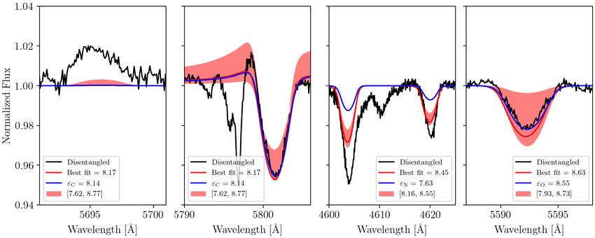
A&A proofs: manuscript no. 9sgr

2017; Mahy et al. 2018), which offer new opportunities to obtain         2. Observations
dynamical mass constraints of stars in the upper mass function.
                                                                         We combine archival and new optical spectroscopy with near-
                                                                         infrared (NIR) interferometry of 9 Sgr. Most of these measure-
    9 Sgr (HD164794) is such a long-period astrometric SB2               ments were part of long-term monitoring programs.
system in the Lagoon Nebula. It was first studied by Abbott et al.
(1984) in the context of its variable synchrotron emission, which
is interpreted to be a result of wind-wind collisions of binaries        2.1. Optical spectra
(Pittard & Dougherty 2006), hinting that the then presumed sin-
gle star 9 Sgr was in fact a binary. Subsequent studies by Rauw          Archival data consist of 57 spectra from the High Efficiency and
et al. (2002a,b) and Nazé et al. (2008) confirmed the presence of        Resolution Mercator Echelle Spectrograph (HERMES, Raskin
elevated X-ray emission, a typical indication of colliding winds         et al. 2011, used in Rauw et al. 2016), 20 Fiber-fed Ex-
in O + O binaries (Rauw et al. 2002c; Sana et al. 2004, 2006;            tended Range Optical Spectrograph (FEROS) spectra (Kaufer
Rauw & Nazé 2016). Rauw et al. (2012) first confirmed the                et al. 1999) and 49 Ultraviolet and Visual Echelle Spectrograph
long-period binary nature of 9 Sgr through radial velocity (RV)          (UVES) spectra (Dekker et al. 2000) in the blue and red arms
measurements and classified its components as O3.5V((f+ )) and           (used in Rauw et al. 2012). Obsrevations that are not previ-
O5.5V((f)). Rauw et al. (2016) studied the periastron passage of         ously analyzed are listed in Table A.1 and consist of five ad-
9 Sgr and reported a maximum in the X-ray emission coming                ditional HERMES spectra and one spectrum from the High Ac-
from shocked gas in the interaction zone of the stellar winds,           curacy Radial velocity Planet Searcher (HARPS) spectrograph
as expected from a wind-wind collision zone in a wide binary             (Mayor et al. 2003). The FEROS spectra cover the spectral do-
where the shocked material cools adiabatically (Stevens et al.           main between 3700 and 9000 Å and have a resolving power of
1992).                                                                   R ≈ 48 000. The UVES spectra cover the wavelength range
                                                                         λλ = 3500 − 5000 Å with its blue arm and λλ = 5000 − 7000 Å
                                                                         with its red arm, and each have a resolving power of R ≈ 40 000.
     The system was resolved for the first time in 2009 us-
                                                                         The HERMES and HARPS spectra both have R ≈ 85 000 with
ing the Astronomical Multi-BEam combineR (AMBER) and in
2013 with the Precision Integrated-Optics Near-infrared Imag-            a coverage of λλ = 3800 − 9000 Å and λλ = 3750 − 6900, re-
ing ExpeRiment (PIONIER) by Sana et al. (2014). Le Bouquin               spectively. The FEROS, UVES, and HARPS spectra were ob-
et al. (2017) constrained the astrometric orbit using multi-epoch        tained through the ESO archive science portal and were pre-
AMBER and PIONIER interferometric measurements, uncov-                   reduced with their respective pipelines. The HERMES spectra
ering a discrepancy with the spectroscopic analyses of Rauw              are reduced using the HERMES Data Reduction Software (DRS)
et al. (2012, 2016). While the interferometric measurements of           pipeline. Finally, all spectra were normalized over their whole
Le Bouquin et al. (2017) firmly excluded inclinations below 80           spectral domain by fitting a cubic spline function through se-
degrees, the RV curve semi-amplitudes of Rauw et al. (2012,              lected continuum regions.
2016) resulted in an estimated inclination of about 50 degrees
if the stars were to have masses representative of their spectral        2.2. Near-infrared Interferometry
types.
                                                                         We used the previously published AMBER and PIONIER
                                                                         dataset obtained from Jun 2009 to Aug 2016 (Le Bouquin et al.
     Another long standing issue is the distance to 9 Sgr, and
                                                                         2017), along with two new PIONIER observations obtained in
whether or not it is a member of the young open cluster
                                                                         May and August 2017. These new data show for the first time
NGC 6530. Prisinzano et al. (2005) and Kharchenko et al. (2005)
                                                                         the system turning back on the apparent ellipse and provide
measured distances to the cluster of around 1.25 kpc, while ear-
                                                                         an almost complete coverage of the nine-year orbit. They were
lier measurements indicated a distance close to 1.8 kpc (van den
                                                                         obtained with PIONIER (Le Bouquin et al. 2011) at the Very
Ancker et al. 1997; Sung et al. 2000) as a result of differences
                                                                         Large Telescope Interferomer (VLTI) using the four 1.8 me-
in the adopted reddening laws. The combination of the astromet-
                                                                         ter Auxiliary Telescopes (ATs) in configurations B2-K0-D0-I3
ric and spectroscopic measurements provide a direct constraint
                                                                         and A0-G1-J2-J3, offering a maximal projected baseline of 120
on the distance, allowing us to confirm the current Gaia eDR3
                                                                         and 130 meter respectively. The PIONIER data were reduced
measurement of 1.21 kpc. Gaia does not suffer from systematics
                                                                         and analyzed, as described in Le Bouquin et al. (2017), us-
owing to an assumed reddening law, and thus provides a power-
                                                                         ing the pndrs1 package. Each observation produces six visi-
ful constraint, but its measurement can still be impacted by the
                                                                         bilities and four closure phases, delivering relative astrometry
multiplicity of the system.
                                                                         with sub-milliarcsecond precision and an H band flux ratio of
                                                                          fH = 0.62 ± 0.02. The full journal of interferometric observa-
    In this work, we aim to resolve the existing discrepant re-          tions is given in Table A.2 along with the measured astrometric
sults that cast doubt on the current mass estimates, evolutionary        properties of the system.
status, and membership of 9 Sgr. To do so, we leverage the ac-                Additionally, three VLTI/GRAVITY (Gravity Collaboration
curacy of relative astrometry and we perform a grid spectral dis-        et al. 2017) measurements were taken, of which two were ob-
entangling analysis on spectroscopic data to fully constrain the         tained in June 2016 and the other in September 2016. These
orbit of 9 Sgr. We further use the atmospheric properties of the         observations were part of the science verification (SV) program
stars in the system to derive its evolutionary status and test stellar   and used the ATs in configurations A0-G1-D0-C1 and A0-G1-
evolution models at high masses. This paper is organized as fol-         J2-K0. As GRAVITY is a spectro-interferometer, it provides six
lows. Section 2 covers the observational data that were used. We         visibilities and four closure phases for each wavelength bin in
present and discuss the orbital analysis and spectral disentan-          the 2.0 − 2.4 µm K band with a spectral resolving power of
gling in Sect. 3, the atmosphere modeling of both components             R = 4000. These SV data were reduced with the standard GRAV-
in Sect. 4, and the evolutionary status of 9 Sgr is discussed in
                                                                         1
Sect. 5. Section 6 presents our conclusions and final remarks.               http://www.jmmc.fr/pndrs

Article number, page 2 of 14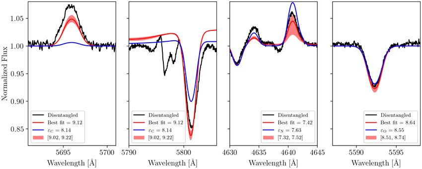
M. Fabry et al.: Resolving the dynamical mass tension of the massive binary 9 Sgr
Table 1: Relative astrometric solution of 9 Sgr, where the usual Table 2: Spectral lines and their respective wavelength ranges
notation of the orbital elements have been adopted (see Ap- that were disentangled to do the grid search described in section
pendix B). The reported errors correspond to the 1σ confidence 3.2.
interval determined by the MCMC analysis.
Spectral line λmin [Å] λmax [Å]
Element [Unit] Value Error He i 4026 4020.0 4031.0
P [d] 3261 69 Hδ 4091.8 4112.5
T 0 [MJD] 56547 12 He ii 4200 4193.0 4206.0
Ω [deg] 67.3 0.4 Hγ 4327.8 4354.5
ω [deg]a 210.7 2.3 He i 4471 4465.0 4477.0
i [deg] 86.5 0.5 He ii 4541 4532.5 4550.0
e 0.648 0.009 He ii 4686 4677.0 4692.0
Notes. (a) By construction, the periastron argument of the relative orbit
Hβ 4841.6 4878.0
ω is shifted by 180◦ compared to the argument of periastron ω1 that is He i 4922 4917.0 4927.0
traditionally adopted by fitting the RV curve of the primary star. He i 5016 5011.0 5026.0
He ii 5411 5399.2 5424.1
ITY pipeline (Lapeyrere et al. 2014, version 1.0.11) and fitted He i 5875 5871.0 5879.5
parametrically to a binary model with PMOIRED2 . The uncer-
tainties on the relative astrometry were estimated by adding a
bootstrapped error and a systematic error of 0.1mas in quadra- In the standard approach, we would fit the profiles of selected
ture. In the bootstrapping procedure, data were drawn randomly spectral lines, or determine the line barycenter, and measure the
to create new datasets and the final parameters and uncertainties red- or blue shift as a function of the observation time to obtain
were estimated as the average and standard deviation of all the an observational RV curve.
fits that were performed. Unfortunately, in this data the spectral However, in long-period systems with broad spectral lines
signal was not of sufficient quality to infer RVs. such as 9 Sgr, the lines of the two components may never fully
deblend, and a small amount of contamination by the other com-
ponent may significantly impact the measured RVs and therefore
3. Orbital analysis the orbital solution and derived masses. Spectral disentangling
can help to improve the measured RVs in this respect because
3.1. Astrometric orbit it is able to account for the cross-contamination of the spec-
The interferometric observations allow us to constrain the or- tral lines of the components. Spectral disentangling however still
bital parameters of the relative orbit, including its orbital period faces challenges when the spectral lines never fully deblend or
(P) and eccentricity (e), by solving for the Thiele-Innes con- when the orbital solution is poorly defined. The most advanced
stants; see Eqs. (B.7)–(B.10). We do so through a Levenberg- spectral disentangling algorithms can optimize the orbital solu-
Marquardt least-squares minimization algorithm implemented in tion at the same time as separating the spectra, but the methods
the newly developed Python package spinOS3 that is described still suffer from degenerate solutions and local minima when ap-
in Appendix B. Errors on each parameter are determined by run- plied to long-period systems as briefly discussed in, for example,
ning a Markov chain Monte Carlo (MCMC) analysis of a hun- Le Bouquin et al. (2017). In this context, we developed another
dred thousand samples. The resulting apparent orbit and orbital approach, that of grid-based spectral disentangling, taking ad-
elements are shown in Fig. 1 and Table 1. The scatterplot matrix vantage of the very precise astrometric solution to drastically re-
of the MCMC analysis is deferred to Fig. A.1. duce the dimensionality of the parameter space that needs to be
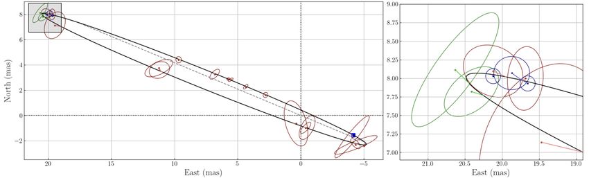
As Le Bouquin et al. (2017) find, the orbit is very well con- explored by spectral disentangling.
strained with a high eccentricity e = 0.648 ± 0.009, a near edge- We base this work on the Fourier disentangling code fd3
on inclination of the orbital plane with the plane of the sky of (formerly FDBinary; Ilijić et al. 2004) by Ilijić (2017). Given the
i = 86.5◦ ± 0.5◦ and an orbital period of P = 8.9 ± 0.2 years. orbital elements (e, P, T 0 , ω, K1 , K2 ), fd3 computes the separated
The scatterplot matrix of the MCMC confirms this solution is spectra independently of any spectral templates. Internally, this
robust (Fig. A.1). Importantly, we corroborate the findings of is achieved by solving a linear least-squares problem introduced
Le Bouquin et al. (2017) that inclinations of 85◦ or lower are by Simon & Sturm (1994), which was reformulated in Fourier
ruled out. space by Hadrava (1995). It is of the form
M x = c, (1)
3.2. Spectral disentangling where x = (x x ) are row vectors representing the (unknown)
A B
separated component spectra xA and xB in Fourier space, c con-
The astrometric solution of Sect. 3.1 only provides the relative tains the Fourier components of the observed composite spectra,
size of the orbit. Determining the absolute size of the orbit inde- and M is the matrix that maps x to c, which depends on the or-
pendently of an assumed distance requires additional informa- bital solution of the system and times of observation. The solver
tion about the system. In the case of 9 Sgr, this information is then uses the singular value decomposition of M as follows:
contained in the Doppler motion of its spectra, specifically, in
the values of the semi-amplitudes of its RV curves (K1 and K2 ). M = UΣVT , (2)
2 and calculates
https://github.com/amerand/PMOIRED
3
https://github.com/matthiasfabry/spinOS x = M−1 c = VΣ−1 UT c. (3)
Article number, page 3 of 14
A&A proofs: manuscript no. 9sgr

Fig. 1: Relative astrometric orbit of 9 Sgr. Archival observations are denoted in red, the new PIONIER data in green, and the
GRAVITY observations in blue, all with their respective error ellipses. The blue square indicates the periastron passage and the
dashed line represents the line of nodes. The right panel shows the zoom-in of the shaded region.

Since M generally has more rows than columns, the system is              perturbed with Gaussian additive noise representative of their
overdetermined and the least-squares solution x1 is returned,            signal-to-noise ratio (S/N). The orbital elements are perturbed
which minimizes the two-norm, and is given by                            with their 1σ error given in Table 1.
                                                                              The considered lines and wavelength ranges are shown in Ta-
      M          c                                                       ble 2. The criteria for selection are that they have high S/N, and
r=        x1 −           ,                                        (4)
      σ          σ   2                                                   that they are absorption lines. Therefore, contrary to the analysis
                                                                         of Rauw et al. (2012), weak metal lines like C iii λ 5696, Si iv λ
which measures how well the orbital elements map the disen-              4116, O iii λ 5592 were neglected owing to their poor S/N with
tangled spectra x1 to the observed spectra c, weighted with its          respect to the deep H and He ii lines.
measurement errors σ.                                                         Performing the fd3 grid disentangling on the lines of Ta-
     Because Fourier transformations are applied, a disadvantage         ble 2 gives the reduced chi-squared contour plot in Fig. 2. We
of this method is that the continuum level of the individual stars       find that the (K1 , K2 ) pair that yields the minimal χ2 value is
is undetermined with respect to the continuum of the composite           K1 = 36 km s−1 , K2 = 49 km s−1 and lies in a rather shallow
spectra. Not only must a flux ratio be supplied to set the individ-      minimum. We used the difference of the (marginalized) 0.84 and
ual contributions to the total flux, but numerical instabilities can     0.16 percentiles of the MC sampling as estimators of the 1σ con-
create large undulations of the disentangled spectra. Therefore,         fidence interval, yielding K1 = 36+4−1 km s , K2 = 49 ± 3 km s ,
                                                                                                                     −1                  −1
the output of the fd3 algorithm must be renormalized again by                                                    +7           +6
                                                                         resulting in dynamical masses of 53−6 M and 39−3 M for the
fitting a smooth function through the regions, where
                                                                         primary and secondary respectively. This differs to the values of
x1 A + x1 B = 1.                                                  (5)    Rauw et al. (2012), who measured K1 = 25.7 ± 0.6 km s−1 and
                                                                         K2 = 38.8 ± 0.9 km s−1 and needed to invoke a much lower in-
    Our novel strategy is to fix the elements (e, P, T 0 , ω) to those   clination to reconcile these with the inferred masses from their
found from the astrometric orbit, and vary K1 and K2 in a grid of        spectral types. While the mass ratio K1 /K2 is similar to our re-
K1 ∈ [15, 45] km s−1 and K2 ∈ [35, 65] km s−1 with 1 km s−1 in-          sults, the semi-amplitude values from Rauw et al. (2012, 2016)
crements. This grid is chosen with the expected total mass from          differ by 30%, that is, more than the statistical uncertainties of
the astrometric orbit and the mass ratio from Rauw et al. (2002a)        the fit. In this sense, in this work we present a different orbital
in mind. We decided to use a flux ratio equal to that observed in        solution. Rauw et al. (2012, 2016) use the mean of the RVs from
the H band, namely f = fH = 0.62. We recorded the reported               the Si iv λ 4116 and N v λλ 4604, 4620 lines for the primary and
reduced chi-squared distance χ2 = r2 of Eq. (4) for each grid            similarly the mean from the He i λλ 4471, 5876, O iii λ 5592,
point, and these are represented in a contour map. We wrapped            C iii λ 5696, and C iv λλ 5801, 5812 lines for the secondary. The
the C code of Ilijić (2017) and the grid setup in a Python package      authors argue that while most of these lines are in fact SB2 lines
available though GitHub4 . Earlier results of this disentangling         (as visible near maximum RV separation), the line blend is dom-
strategy were presented on other challenging systems (Shenar             inated by only one component such that they treated them as
et al. 2020; Bodensteiner et al. 2020).                                  SB1 lines tracing only the motion of that component. The spec-
    Instead of running the above procedure on the full wave-             tral disentangling results however show that both components
length domain of the spectra, which would be computationally             contribute to these lines, sometimes significantly. For example,
expensive, we selected strong spectral lines and did the anal-           Fig A.4 shows the O iii λ 5592 line, to which the primary con-
ysis on these lines separately. We then summed the obtained              tributes about 25% as compared to the total depth of the line. As
chi-squared distances, and reduced them by dividing with the             discussed in Sana et al. (2011) and quantitatively investigated
summed degrees of freedom, effectively clipping unwanted con-            in Bodensteiner et al. (2021, in press), the effect may be more
tinuum regions. The errors were estimated by a Monte Carlo               subtle than this example because an even smaller contamination
(MC) sampling analysis, in which we drew 1500 samples of                 impacts the measured RVs. While for many systems this is of
the full grid disentangling procedure, where the spectra are             minor importance, in the present case, even a bias as small as
                                                                         5 km s−1 on the RVs is large (∼10%) compared to the measured
4
    https://github.com/matthiasfabry/gridfd3                             semi-amplitudes.
Article number, page 4 of 14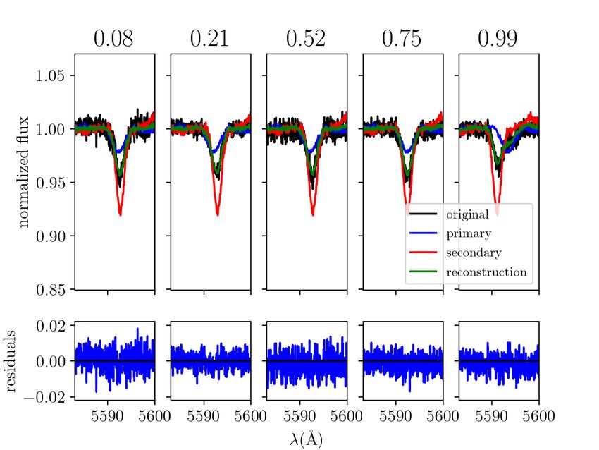
M. Fabry et al.: Resolving the dynamical mass tension of the massive binary 9 Sgr

                                                                       Table 3: Results of the fd3 grid search for the RV semi-
                                                                       amplitudes. Column two gives the grid point that has the min-
                                                                       imal reduced chi-squared value when disentangling the original
                                                                       data. Columns 3, 4 and 5 give the MC median and 1σ confidence
                                                                       intervals.

                                                                             Semi-amplitudes       Data     MC median       σ−     σ+
                                                                               K1 (km s−1 )         36         36           35     40
                                                                               K2 (km s−1 )         49         50           47     53

                                                                       fication of the primary by Rauw et al. (2012) from O3.5V((f+ ))
                                                                       to O3V((f+ )), and narrow down the subtype of the secondary
                                                                       from O5-5.5V((f)) to O5V((f)). This is in excellent agreement
                                                                       with the recent work of Quintero et al. (2020), who used an
                                                                       updated version of the shift-and-add disentangling technique in
                                                                       wavelength space and also obtained spectral types of O3V((f+ ))
                                                                       and O5V((f)).
Fig. 2: Reduced chi-squared contour map of the grid disen-                 To confirm the quality of the disentangling procedure, we re-
tangling combining all lines of Table 2. The minimal χ2red , at        combine the disentangled spectra at various phases and compute
K1 = 36 km s−1 , K2 = 49 km s−1 , is denoted with a red dot. The       residuals. To avoid mixing different instrumental wavelength
solid red and orange lines represent the 1σ and 2σ contours re-        calibrations, only the HERMES spectra are used. Reconstructed
spectively, after scaling the χ2 map so that the minimum satisfies     lines are shown in Figs. A.3 and A.4. The average residuals of
χ2red = 1.                                                             the reconstructed lines to the original composite spectra are on
                                                                       the order 1%. While very good, this is larger than expected from
                                                                       pure S/N considerations and probably results from small uncer-
                                                                       tainties in the normalization of individual spectra that impacts
                                                                       the disentangling results of fd3.

                                                                       3.3. Distance
                                                                       Because the semi-amplitudes K1 and K2 set the absolute scale of
                                                                       the orbit, we can infer the distance to 9 Sgr by measuring against
                                                                       the apparent orbit found through the interferometry (Fig. 1), via
                                                                       the total mass of the system and Kepler’s third law, as follows:
                                                                                  r
                                                                             1 3 G(M1 + M2 )P2
                                                                       d=                           ,                                 (6)
                                                                            aapp          4π2
                                                                       where aapp is the semimajor axis of the apparent orbit in angular
                                                                       units. The values (K1 , K2 ) = (36, 49) km s−1 correspond to a total
                                                                       dynamical mass of 92 M , which results in a distance of
                                                                       d = 1310 ± 60 pc,                                                 (7)
Fig. 3: Two-dimensional histogram of the results of the MC sam-        where we propagated the MC errors.
pling in (K1 , K2 ) space. The color indicates the number of sam-          This value lies within the Gaia eDR3 geometric distance re-
ples N at the corresponding (K1 , K2 ) pairs. The result from the      ported by Bailer-Jones et al. (2020) of 1218+100
original data is encircled in red.                                                                                    −108 pc. With these
                                                                       results, it seems likely that 9 Sgr is a member of NGC6530,
                                                                       confirming the measurements of Prisinzano et al. (2005) and
                                                                       especially Kharchenko et al. (2005), who quoted a distance of
    The results of the fd3 grid search are summarized in Ta-           d = 1322 pc. Conversely, we can firmly exclude distances to
ble 3. The error analysis shows K1 has a slightly asymmetric 1σ        9 Sgr of over 1500 pc because that would require a total mass
uncertainty, as indicated in Table 3 and shown in the 2D (K1 , K2 )    of over 130M , which our grid disentangling results do not sup-
histogram in Fig. 3. Yet, for both K1 and K2 , the median of the       port. Similarly, the distance of 1780 ± 80 pc of Sung et al. (2000)
retrieved MC values lies within 1σ of the input value, giving us       adopted by Rauw et al. (2012) is incompatible with the interfer-
confidence in the accuracy of the method. For comparison, the          ometric and Gaia measurements of the apparent size of the orbit
marginalized histograms are shown in Fig. A.2.                         and the derived component masses.
    We show the broad range disentangled spectra in Fig. 4.
From visual inspection of the line depth ratio of He i λ 4471
to He ii λ 4541, we immediately notice that the primary is the         4. Atmosphere modeling
hottest star of the two. This fact is seen in the N v λλ 4604,         4.1. Setup
4620 lines as well. Comparing equivalent widths of lines in
the disentangled spectra with classification tables of Conti &         Using the disentangled spectra, we adjust theoretical line pro-
Alschuler (1971) and Sana et al. (in prep.), we update the classi-     files computed with the fastwind NLTE atmosphere code suit-
                                                                                                                 Article number, page 5 of 14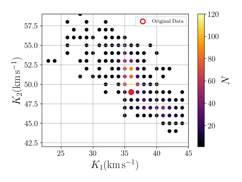
A&A proofs: manuscript no. 9sgr

Fig. 4: Disentangled, renormalized spectra of both components using K1 = 36 km s−1 and K2 = 49 km s−1 . The spectrum of the
primary is shifted up by 0.4 units with respect to the secondary for clarity. In Hα, the core is contaminated by nebular emission
present in the FEROS and HERMES spectra. The model spectra are those obtained with the best-fit atmospheric parameters from
the fastwind analysis (Sect. 4).

able for the expanding atmosphere of O-type stars (Santolaya-           Micron All-Sky Survey (2MASS, Skrutskie et al. 2006), giving
Rey et al. 1997; Puls et al. 2005; Carneiro et al. 2016; Puls 2017;     an apparent magnitude in the near-infrared KS band of mKS =
Sundqvist & Puls 2018). To reduce the dimensionality of the pa-         5.731 ± 0.024 for the total system. Using the interstellar absorp-
rameter space, the rotational and macroturbulent velocities are         tion coefficient AV = 1.338 ± 0.021 from Maíz Apellániz &
estimated using the iacob-broad tool (Simón-Díaz & Herrero              Barbá (2018), the color correction AKS /AV = 0.116 from Fitz-
2014). Analyzing (with the goodness-of-fit method) the O iii λ          patrick (1999) and a distance of 1.31 ± 0.06 kpc calculated in
5592 and N v λ 4603 lines for the primary and O iii λ 5592, He i        Sect. 3.3 results in an absolute magnitude in the KS band of
λ 4713 and He i λ 5876 for the secondary, we find a projected           MKS = −5.01 ± 0.10. We correct for the measured PIONIER flux
rotational velocity v sin i = 102+8
                                  −12 km s
                                           −1
                                              and a macroturbulent      ratio f = 0.62 between the components, where we assume that it
                    +23
velocity vmac = 77−20 km s for the primary star, while we take
                             −1                                         remains unchanged between the H and KS band (as expected for
v sin i = 67+6       −1
                        and vmac = 48+21       −1                       such hot objects). This yields absolute component magnitudes
            −13 km s                  −14 km s    for the secondary.
Similar values are obtained when using the Fourier transform            of MKS = −4.49 ± 0.10 and −3.96 ± 0.10 for the primary and
method.                                                                 secondary, respectively. We note that these values correspond to
     The stellar atmosphere models are then iterated using a ge-        fainter stars than their derived spectral types suggest. Synthetic
netic algorithm (Charbonneau 1995; Mokiem et al. 2005) within           photometry of Martins & Plez (2006) give MK = −4.98 and
a predefined parameter space to optimize a χ2 fitness metric until      MK = −4.39 for the O3V primary and O5V secondary, respec-
a convergence to the best fit with the spectrum is reached. The         tively, which suggests the stars are slightly more compact.
version of the genetic algorithm used is detailed in Abdul-Masih
et al. (2019). We set the β exponent of the wind acceleration law
to 0.85, as appropriate for main-sequence stars (Muijres et al.         4.2. Results and discussion
2012). The microturbulence velocity is fixed to vmic = 10 km s−1
in the computation by fastwind; in the formal integral it is se-        We list the spectroscopic parameters of the resulting best-fit at-
lected on the criteria vmic = max(10 km s−1 , 0.1vwind ). We include    mospheric models and the resulting inferred parameters in the
optically thin wind clumping, with a near constant clumping fac-        leftmost column of Table 4. The corresponding theoretical spec-
tor fcl throughout the wind. Lastly, we opted to clip the core of       tra are plotted in Fig. 4 with dashed lines. We note the obvious
the Hα line to avoid fitting the nebular emission remnant (visi-        nebular contamination of Hα, as well as the general trend that
ble in the bottom-rightmost panel of Fig. 4). The full list of fitted   the disentangled spectra are slightly shallower than the model
spectral lines is shown in Table A.3.                                   spectra in the deep and broad lines (like Hδ, Hγ and He ii λ
     To provide an absolute magnitude anchor point for the at-          4686), suggesting issues in the normalization of these broad
mospheric model, we adopt the photometric data from the Two             lines.
Article number, page 6 of 14
M. Fabry et al.: Resolving the dynamical mass tension of the massive binary 9 Sgr
The best-fit parameters depend on which line features were find that the evolutionary masses are within error of the dynami-
considered in the fit and with what weights. For example, giving cal masses, which provides a further indication that the spectro-
more weight to He i lines would result in lower inferred effec- scopic mass likely suffers from systematic errors. Additionally,
tive temperatures and vice versa. Correspondingly, the inferred the evolutionary models favor lower CNO surface abundances
surface gravities would be lower for lower T eff and vice versa. than are spectroscopically inferred, especially nitrogen in the pri-
Therefore, conservative errors of 1kK and 0.2 dex on T eff and mary and carbon in the secondary. The rather modest rotational
log g, respectively, are adopted. Furthermore, the determination velocities and young ages do not allow for rotational mixing to
of the quality of the CNO abundance measurements is challeng- modify the surface composition; the CNO abundances returned
ing. The carbon abundance for the secondary, for example, is fit- by bonnsai correspond to the baseline value of the Brott et al.
ted to [C/H] + 12 = 9.12; this is an unusually high measurement (2011) models with very small uncertainties.
that has (to our knowledge) never before been observed. We note From the atmosphere models in Table 4, it is clear that the
that this measurement is driven by the C iii λ 5696 line, which is CNO composition between the primary and the secondary is dif-
in emission. At T eff = 42kK, fastwind can only reconcile this ferent. This is not reflected in the evolutionary tracks because
line in emission by boosting the carbon abundance. Keeping the both models prefer the baseline values of the Brott et al. (2011)
issues presented by this line in mind, however (see Martins & tracks, namely [C/H] + 12 = 8.13, [N/H] + 12 = 7.64 and
Hillier 2012), we adopt the minimum of a formal 0.1 dex error [O/H] + 12 = 8.55 (middle column of Table 4). Furthermore,
and the statistical error of the grid of models. Since this for- if we assume the abundances of the secondary are baseline for
mal error is somewhat arbitrary, even these uncertainties should 9 Sgr, this source has a different CNO baseline than the Brott
be interpreted with great care. Therefore we can only argue for et al. (2011) tracks. It is hard to justify observationally that the
qualitative enrichment of nitrogen in the primary and enrichment observed abundances of the secondary are baseline for 9 Sgr or
of carbon in the secondary. For added justification, we show in the cluster NGC6530. But we expect the least massive star with
Figs. A.5 and A.6 the comparison of the model spectra, their er- the lowest rotational velocity to be least contaminated by surface
ror ranges along with spectra using the Brott et al. (2011) CNO enrichment from a theoretical standpoint. We thus test if bonn-
baseline abundances in various diagnostic lines of the CNO ele- sai finds different models for the primary if we scale down the
ments. observed CNO abundances to the Brott et al. (2011) baseline.
The best-fit log g values then provide the spectroscopic For the abundances of the primary to maintain the same frac-
masses of the stars, which are found to be 32 ± 16M and tional difference versus the secondary, this amounts to calculat-
19 ± 10M for the primary and secondary, respectively. These ing [X 0 /H] = [X/H]base,Brott − [X/H]base,obs + [X/H]prim,obs . Keep-
masses are significantly lower than their dynamical counterparts, ing the doubtful C abundance measurement of the secondary
albeit with large error bars, and are not representative of dwarf in mind (Sect. 4.2), we refrain from scaling C and compute
stars of that luminosity. The main reason for this discrepancy is [N0 /H] + 12 = 8.67+0.14 +0.14
−0.31 and [O /H] + 12 = 8.54−0.71 . Using
0
the low inferred log g, which should be raised by about 0.25 dex then again log L, T eff , XHe , and v sin i from the fastwind models,
for both stars, that is, slightly beyond the adopted uncertainty, along with these new N and O abundances as input for bonn-
to match the dynamical masses. The mass discrepancy problem sai, we obtain other highest likelihood evolutionary parameters;
(Herrero et al. 1992) is still an open issue in massive-star spec- these are listed in the rightmost column of Table 4. These results
troscopy, and while more recent studies (e.g., Mahy et al. 2020) point to a different scenario. Here the rotational velocity is sig-
show that for stars above ∼35M , the discrepancy largely dis- nificantly higher, allowing significant rotational mixing to occur.
appears, in this analysis, it is still present. The repeated normal- The primary age has increased to match that of the secondary as
ization of the spectra before and after disentangling could be the well, while the evolutionary mass, log g and T eff are only slightly
root cause of this fact, as the reconstruction plots in Fig. A.3 changed when comparing to the nonscaled results (middle col-
and A.4 and the comparison to the model spectra (Fig. 4) hint umn of Table 4). The major implication of this is that either the
towards. rotational axis and the normal to orbital plane are heavily in-
clined, up to an estimated 68 degrees to explain the observed
projected rotational velocity, or the effect of rotational mixing
5. Evolutionary modeling is underestimated in the stellar evolution models. We cannot ex-
clude either that a mixing mechanism weakly dependent on ro-
We compare our previous results with the Milky Way evolu-
tation is operating on stars in this mass regime. Distinguishing
tionary tracks of Brott et al. (2011), using the Bayesian search
between these scenarios however requires greater confidence in
tool bonnsai5 (Schneider et al. 2014). The bonnsai tool allows us
the quality of the CNO abundance measurements.
to search the rotating single star evolution tracks of Brott et al.
We summarize our results of Sects. 4 and 5 in an HRD and
(2011) for the highest likelihood stellar model that corresponds
a Kiel diagram that is overplotted on several of the evolution-
to measured quantities. We input the observed log L, T eff , XHe ,
ary tracks and isochrones of Brott et al. (2011). We note that
and v sin i from the left column of Table 4 and request the high-
while the location of the models on the HR diagram matches
est likelihood models of both stars in the grid. To avoid biasing
well, there is a mismatch of the spectroscopic mass inferred from
the Bayesian search, we refrain from using the log g due to the
the fastwind models and the evolutionary masses. In the Kiel di-
uncertainties posed by the mass discrepancy. In a first search, we
agram, there is a poorer match as expected from the mass dis-
do not input the CNO abundances obtained from fastwind. The
crepancy discussed in Sect. 4.2.
parameters from the highest likelihood models replicated from
our spectroscopic and photometric observables of this search are
given in the middle column of Table 4. 6. Conclusions
The comparison with evolutionary tracks point toward rela-
tively compact and coeval stars with an age of about 1 Myr. We We have obtained disentangled spectra of 9 Sgr using a com-
bination of high angular resolution astrometry and spectral grid
5
The BONNSAI web-service is available at www.astro.uni- disentangling with the fd3 code. The astrometric measurements
bonn.de/stars/bonnsai. solidify the long period of 8.9 yr and have a near edge-on in-
Article number, page 7 of 14A&A proofs: manuscript no. 9sgr
Table 4: Parameters of the best-fit, genetically evolved fastwind atmospheric model (described in Sect. 4), along with replicated
observables from the Brott et al. (2011) models using bonnsai (Sect. 5). The errors correspond to the 1σ confidence level. Empty
entries are indeterminable for that parameter.
fastwind bonnsai
Parameter(Unit) Primary Secondary Primary Secondary Primary, Scaled CNO
T eff [kK] 46.0 ± 1.0 42.0 ± 1.0 45.9+0.6
−0.9 41.9 ± 0.9 46.0+0.6
−1.0
log(g/[cgs]) 3.87 ± 0.20 3.87 ± 0.20 4.11 ± 0.05 4.12+0.06
−0.07 4.10 +0.02
−0.06
log M Ṁ/yr −6.6 ± 0.2 −6.6 ± 0.2 ... ... ...
fcl 29 ± 5 22 ± 3 ... ... ...
v sin i [km s−1 ]a 102+8
−12 67+6
−13 ... ... ...
vrot [km s−1 ] ... ... 110+59
−26
+8
70−15 330+26
−30
YHe 0.25 ± 0.04 0.24 ± 0.03 0.26b 0.26 b
0.28+0.08
−0.02
[C/H] + 12 8.17+0.60
−0.55 9.12 ± 0.10* 8.14+0.01
−0.03 8.13b 7.12+0.55
−0.05
[N/H] + 12 +0.10
8.45−0.29 7.42 ± 0.10 7.63+0.09
−0.01 7.64 b
8.72+0.10
−0.27
[O/H] + 12 8.63+0.10
−0.70 8.64+0.10
−0.13 8.55+0.01
−0.02 8.55b 8.55+0.01
−0.61
log(L/L ) 5.68 ± 0.08 5.35 ± 0.08 5.64+0.07
−0.06 5.33+0.08
−0.06 5.67 +0.06
−0.07
R [R ] 10.8 ± 1.0 8.9 ± 1.2 10.45+0.88
−0.59 8.73+0.75
−0.67 10.73+0.79
−0.61
Mspec [M ] 32.1 ± 16.0 18.9 ± 10.1 ... ... ...
Mevol [M ] ... ... 53.4+3.2
−3.3 37.0+2.0
−2.3 53.8 ± 4.7
Age [Myr] ... ... 0.52+0.32
−0.33
+0.48
1.00−0.58 1.00+0.80
−0.41
Notes. (a) Determined using iacob-broad, not fastwind. (b)
Very small error, see Sect. 5. (*)
Highly uncertain measurement, this formal error is
likely not representative, see Sect. 4.2.
clination of 86.5 degrees. Our results confirm the presence of Abdul-Masih, M., Sana, H., Sundqvist, J., et al. 2019, ApJ, 880, 115
an O3V+O5V massive binary, which has inferred dynamical Bailer-Jones, C. A. L., Rybizki, J., Fouesneau, M., Demleitner, M., & Andrae,
R. 2020, ArXiv201205220 Astro-Ph
masses of about 53 and 39 M , making 9 Sgr one of the most Bodensteiner, J., Sana, H., Wang, C., et al. 2021, ArXiv210413409 Astro-Ph
massive galactic O+O binaries ever resolved. Furthermore, to Bodensteiner, J., Shenar, T., Mahy, L., et al. 2020, A&A, 641, A43
our knowledge, this is only the second instance of a dynamical Brott, I., de Mink, S. E., Cantiello, M., et al. 2011, A&A, 530, A115
mass estimate of a galactic O3V star (the other from Mahy et al. Carneiro, L. P., Puls, J., Sundqvist, J. O., & Hoffmann, T. L. 2016, A&A, 590,
2018). A88
Charbonneau, P. 1995, AJSS, 101, 309
By re-deriving the semi-amplitudes of the RV curves, we Conti, P. S. & Alschuler, W. R. 1971, AJ, 170, 325
clear up the contradictory results between the previous RV mea- Dekker, H., D’Odorico, S., Kaufer, A., Delabre, B., & Kotzlowski, H. 2000, in
surements of Rauw et al. (2012) and the high inclination of the Optical and IR Telescope Instrumentation and Detectors, Vol. 4008 (Interna-
interferometric orbit by Le Bouquin et al. (2017). Furthermore, tional Society for Optics and Photonics), 534–545
Fitzpatrick, E. L. 1999, PASP, 111, 63
the results show 9 Sgr is a member of the young open cluster Gravity Collaboration, Abuter, R., Accardo, M., et al. 2017, A&A, 602, A94
NGC 6530. The combined dynamical, atmospheric, and evolu- Hadrava, P. 1995, A&AS, 114, 393
tionary modeling shows 9 Sgr contains massive stars of roughly Herrero, A., Kudritzki, R. P., Vilchez, J. M., et al. 1992, A&A, 261, 209
53M and 37M for the primary and secondary, respectively. Hilditch, R. W. 2001, An Introduction to Close Binary Stars (Cambridge Univer-
sity Press)
9 Sgr is a unique system in the far top left corner of the HRD, Ilijić, S. 2017, ASCL, ascl:1705.012
and therefore provides an equally unique opportunity to use its Ilijić, S., Hensberge, H., Pavlovski, K., & Freyhammer, L. M. 2004, ASPC, 318,
stellar and systemic parameters to compare with massive star 111
evolutionary models as well as binary formation scenarios. Kaufer, A., Stahl, O., Tubbesing, S., et al. 1999, The Messenger, 95, 8
Kharchenko, N. V., Piskunov, A. E., Röser, S., Schilbach, E., & Scholz, R.-D.
Acknowledgements. This project has received funding from the European Re- 2005, A&A, 438, 1163
search Council (ERC) under the European Union’s Horizon 2020 research and Lapeyrere, V., Kervella, P., Lacour, S., et al. 2014, in Society of Photo-Optical
innovation programme (grant agreement number DLV-772225-MULTIPLES), Instrumentation Engineers (SPIE) Conference Series, Vol. 9146, Proc. SPIE,
the KU Leuven Research Council (grant C16/17/007: MAESTRO), the FWO 91462D
through a FWO junior postdoctoral fellowship (No. 12ZY520N) as well as the Le Bouquin, J.-B., Berger, J.-P., Lazareff, B., et al. 2011, A&A, 535, A67
European Space Agency (ESA) through the Belgian Federal Science Policy Of- Le Bouquin, J.-B., Sana, H., Gosset, E., et al. 2017, A&A, 601, A34
fice (BELSPO). Based on observations obtained with the HERMES spectro- Mahy, L., Almeida, L. A., Sana, H., et al. 2020, A&A, 634, A119
graph, which is supported by the Research Foundation - Flanders (FWO), Bel- Mahy, L., Gosset, E., Manfroid, J., et al. 2018, A&A, 616, A75
gium, the Research Council of KU Leuven, Belgium, the Fonds National de la Maíz Apellániz, J. & Barbá, R. H. 2018, A&A, 613, A9
Recherche Scientifique (F.R.S.-FNRS), Belgium, the Royal Observatory of Bel- Maíz Apellániz, J., Sana, H., Barbá, R. H., Le Bouquin, J.-B., & Gamen, R. C.
gium, the Observatoire de Genève, Switzerland and the Thüringer Landesstern- 2017, MNRAS, 464, 3561
warte Tautenburg, Germany. Martins, F. & Hillier, D. J. 2012, A&A, 545, A95
Martins, F. & Plez, B. 2006, A&A, 457, 637
Mayer, P., Harmanec, P., Sana, H., & Le Bouquin, J.-B. 2014, AJ, 148, 114
Mayor, M., Pepe, F., Queloz, D., et al. 2003, The Messenger, 114, 20
References Mokiem, M. R., de Koter, A., Puls, J., et al. 2005, A&A, 441, 711
Muijres, L. E., Vink, J. S., de Koter, A., Müller, P. E., & Langer, N. 2012, A&A,
Abbott, D. C., Bieging, J. H., & Churchwell, E. 1984, ApJ, 280, 671 537, A37
Article number, page 8 of 14M. Fabry et al.: Resolving the dynamical mass tension of the massive binary 9 Sgr
Schneider, F. R. N., Langer, N., de Koter, A., et al. 2014, A&A, 570, A66
Shenar, T., Bodensteiner, J., Abdul-Masih, M., et al. 2020, A&A, 639, L6
Simon, K. P. & Sturm, E. 1994, A&A, 281, 286
Simón-Díaz, S. & Herrero, A. 2014, A&A, 562, A135
Skrutskie, M. F., Cutri, R. M., Stiening, R., et al. 2006, AJ, 131, 1163
Stevens, I. R., Blondin, J. M., & Pollock, A. M. T. 1992, AJ, 386, 265
Sundqvist, J. O. & Puls, J. 2018, A&A, 619, A59
Sung, H., Chun, M.-Y., & Bessell, M. S. 2000, AJ, 120, 333
van den Ancker, M. E., The, P. S., Feinstein, A., et al. 1997, A&AS, 123, 63
Fig. 5: Top: Hertzsprung-Russell diagram, showing the location
of the best-fit fastwind models (FW) and highest likelihood evo-
lutionary models from Brott et al. (2011) (bonnsai). Overplotted
are evolutionary tracks for different masses and initial rotation
velocities (grey lines), along with isochrones for the 100km s−1
initial rotation velocity models (blue lines). Bottom: Kiel dia-
gram with an equivalent legend as the HRD above. Using the
scaled CNO abundances does not appreciably move the model
of the primary in either diagram.
Nazé, Y., Becker, M. D., Rauw, G., & Barbieri, C. 2008, A&A, 483, 543
Newville, M., Otten, R., Nelson, A., et al. 2020, Lmfit/Lmfit-Py 1.0.1, Zenodo
Pittard, J. M. & Dougherty, S. M. 2006, MNRAS, 372, 801
Prisinzano, L., Damiani, F., Micela, G., & Sciortino, S. 2005, A&A, 430, 941
Puls, J. 2017, in Proceedings IAU Symposium, Vol. 329, 435–435
Puls, J., Urbaneja, M. A., Venero, R., et al. 2005, A&A, 435, 669
Quintero, E. A., Eenens, P., & Rauw, G. 2020, Astron. Nachrichten, 341, 628
Raskin, G., van Winckel, H., Hensberge, H., et al. 2011, A&A, 526, A69
Rauw, G., Blomme, R., Nazé, Y., et al. 2016, A&A, 589, A121
Rauw, G., Blomme, R., Waldron, W. L., et al. 2002a, A&A, 394, 993
Rauw, G. & Nazé, Y. 2016, AdSpR, 58, 761
Rauw, G., Nazé, Y., Gosset, E., et al. 2002b, A&A, 395, 499
Rauw, G., Sana, H., Spano, M., et al. 2012, A&A, 542, A95
Rauw, G., Vreux, J.-M., Stevens, I. R., et al. 2002c, A&A, 388, 552
Sana, H., Bouquin, J.-B. L., Lacour, S., et al. 2014, ApJS, 215, 15
Sana, H., Le Bouquin, J.-B., De Becker, M., et al. 2011, ApJL, 740, L43
Sana, H., Le Bouquin, J.-B., Mahy, L., et al. 2013, A&A, 553, A131
Sana, H., Rauw, G., Nazé, Y., Gosset, E., & Vreux, J.-M. 2006, MNRAS, 372,
661
Sana, H., Stevens, I. R., Gosset, E., Rauw, G., & Vreux, J.-M. 2004, MNRAS,
350, 809
Santolaya-Rey, A. E., Puls, J., & Herrero, A. 1997, A&A, 323, 488
Article number, page 9 of 14A&A proofs: manuscript no. 9sgr
Appendix A: Additional tables and figures
Table A.1: Previously unanalyzed spectra of 9 Sgr. The columns signify the modified Julian date (MJD) of observation, spectro-
graph, exposure time and estimated S/N at 4500Å.
MJD Instrument exposure time (s) S/N
57171.1874 HERMES 571 90
57172.1426 HERMES 325 96
57173.1646 HERMES 478 75
57201.0247 HERMES 360 138
57236.9486 HERMES 800 161
57634.0119 HARPS 180 143
Table A.2: Journal of the interferometric measurements of 9 Sgr. Given are the VLTI instrument (Instr.), the MJD of observation,
the relative angular separation (Sep.), the position angle (PA) east of north, and the major (σmaj ) and minor (σmin ) axes of the 1σ
error ellipses along with its PA east of north (PAσ ).
Instr. MJD Sep. (mas) PA (deg) σmaj (mas) σmin (mas) PAσ (deg)
AMBER 54995.306 20.74 69.87 1.12 0.75 154
AMBER 55644.304 11.85 71.58 1.20 0.50 116
AMBER 55648.389 11.76 72.19 0.83 0.63 113
PIONIER 56154.134 0.74 149.10 1.85 0.82 16
PIONIER 56189.027 1.09 207.39 1.03 0.48 153
PIONIER 56191.087 1.05 201.56 0.57 0.21 138
PIONIER 56376.318 4.87 242.59 0.50 0.23 44
PIONIER 56383.324 4.94 241.83 1.82 0.31 112
PIONIER 56438.244 5.57 244.91 0.13 0.06 151
PIONIER 56549.143 4.40 247.37 2.12 0.36 141
PIONIER 56714.359 3.23 59.89 0.21 0.18 150
PIONIER 56751.389 4.92 62.51 0.24 0.10 135
PIONIER 56783.350 6.23 63.05 0.22 0.09 121
PIONIER 56787.340 6.43 63.33 0.12 0.09 127
PIONIER 56818.282 7.56 64.46 0.50 0.23 137
PIONIER 56903.045 10.63 65.49 0.25 0.22 6
PIONIER 57558.303 21.25 67.89 0.43 0.24 176
GRAVITY 57558.305 21.194 68.028 0.101 0.102 90
GRAVITY 57560.312 21.45 67.90 0.24 0.22 90
GRAVITY 57647.081 21.664 68.246 0.101 0.102 90
PIONIER 57601.215 21.69 68.08 0.42 0.33 62
PIONIER 57900.386 22.17 68.53 0.93 0.27 144
PIONIER 57995.105 21.86 69.04 0.43 0.25 130
Article number, page 10 of 14M. Fabry et al.: Resolving the dynamical mass tension of the massive binary 9 Sgr
Fig. A.1: Scatterplot matrix of the MCMC sampling of the orbital solution minimization in section 3.1. While the expected heavy
T 0 − ω correlation is apparent, no unexpected degeneracies in the parameter space are observed.
Fig. A.2: Marginalized histograms of the MC error analysis in Sect. 3.2.
Article number, page 11 of 14A&A proofs: manuscript no. 9sgr
Table A.3: Spectral lines and their respective wavelength ranges, which were fitted against the fastwind atmosphere modeling in
Sect. 4, for the primary and secondary star.
Spectral line λmin [Å] λmax [Å]
He i 4026 4022.0 4029.8
N iv 4058 4056.5 4059.9
Hδ 4093.6 4107.9
He ii 4200 4195.5 4204.3
Hγ 4332.5 4348.4
He i 4471 4468.6 4474.0
He ii 4541 4535.5 4547.3
N v 4604 4600.3 4608.5
N v 4619 4617.4 4622.8
He ii 4686 4680.6 4690.4
Hβ 4850.8 4870.9
He ii 5411 5405.4 5417.1
O iii 5592 5589.3 5595.4
C iii 5696 5692.4 5698.8
C iv 5801 5798.8 5805.0
C iv 5812 5809.3 5815.0
He i 5875 5872.0 5878.9
Hα 6551.7 6571.2
Fig. A.3: Reconstruction of the Hδ line at orbital phases in- Fig. A.4: Reconstruction of the O iii 5592 line at orbital phases
dicated above each column. At phase 0.99 the reconstruction indicated above each column. A good correspondence is ob-
is slightly too shallow (∼1%) near the core, hinting at a pos- served, even for this relatively weak metal line, although the
sible inconsistent normalization across the spectra. The well reconstruction is slightly too shallow at phase 0.99.
resolved N iii feature in the left wing of Hδ is noted.
Article number, page 12 of 14M. Fabry et al.: Resolving the dynamical mass tension of the massive binary 9 Sgr
Fig. A.5: Comparison of the disentangled and best-fit model spectra of the primary star with error ranges, along with a model
spectrum having the Brott et al. (2011) CNO baseline abundances. From left to right, the lines C iii λ 5696, C iv λ 5801, N v λλ
4604, 4620, and O iii 5592 are shown, and the legend stipulates the respective CNO abundance values [X/H]+12 and the baseline
values εX . As these lines are the main abundance diagnostic for their respective CNO element, from the third panel it can be seen
that there is evidence for significant nitrogen enrichment.
Fig. A.6: Comparison of the disentangled and best-fit model spectra of the secondary star with error ranges, along with a model
spectrum having the Brott et al. (2011) CNO baseline abundances. From left to right, the lines C iii λ 5696, C iv λ 5801, N iii λλ 4634,
4641, and O iii 5592 are shown, with a similar legend as Fig. A.5. The two leftmost panels argue for an elevated carbon abundance
with respect to baseline, although as discussed in Sect. 4.2, the issues of C iii λ 5696 prohibits making quantitative conclusions.
Article number, page 13 of 14A&A proofs: manuscript no. 9sgr
Appendix B: spinOS Given then a set of measurements RV1obs (ti ), RV2obs (t j )
and ∆Nobs (tk ), ∆Eobs (tk ), we minimize the objective function,
In this appendix, we introduce spinOS, a modern Python imple- which doubles as a chi-squared measure of the goodness of fit.
mentation of an orbital minimization algorithm. The 3D orbit of Schematically it is given by
a binary system can be obtained through two independent sets of
measurements: RV measurements via Doppler spectroscopy and X O(ti ) − C(ti ; ϑ) !2
apparent separations through interferometric or visual astrome- χ2 (ϑ) = , (B.13)
try. i
σ(ti )
We assume the motion of the bodies is governed by Newton’s
equations and thus Kepler’s laws hold (i.e., we neglect all rela- where O and C are observed and computed data, σ the error on
tivistic effects). Both components then follow ellipses described the observations, and ϑ symbolizes the set of orbital parameters.
by their radius vector with respect to the common focal point We use the Levenberg-Marquardt minimization algorithm im-
r(t), which is a function of time t and is dependent on the orbital plemented by the package lmfit (Newville et al. 2020) to find
elements the orbital parameters ϑ that minimize eq. (B.13). By default, er-
rors are estimated from the diagonal elements of the covariance
r(t) = r(t; K, e, i, ω, Ω, T 0 ), (B.1) matrix, but, an MCMC option is available that takes correlations
where K = 2πa
√ sin i
is the semi-amplitude of the RV curve, P the between parameters into account. In the latter, a specified num-
P 1−e2 ber of samples is drawn around the minimum to obtain an ap-
orbital period, a the semimajor axis, e the eccentricity, i the incli-
proximated posterior probability distribution of the parameters,
nation of the orbital plane with respect to the sky, ω the argument
of which different quantile masses define different confidence
of periastron, Ω the longitude of the ascending node, and T 0 the
intervals.
time of periastron passage. In the optimal case in which astrom-
Finally, we present the orbital modeling and minimization
etry and RVs are available, we can determine all the elements as
routine in a user friendly graphical user interface constructed
well as the distance to the system. If we only have astrometry,
using tkinter, where the user chooses, among others, which
the (sum of the) semi-amplitudes are degenerate with the dis-
data to be plotted, which orbital parameters to fit for, and which
tance. Conversely, if we have only RVs of either or both of the
weights to give the astrometry relative to the spectroscopic mea-
components, the inclination and longitude of the ascending node
surements. The spinOS tool is available under a GNU GPL 3.0
and the distance remain unconstrained.
(or later) license through GitHub on https://github.com/
The RV equation, which measures the velocity of an orbital
matthiasfabry/spinOS.
component along the normal of the plane of the sky (≡ z-axis),
is well known and reduces to (see, e.g., Hilditch 2001)
RV(t) = ż(t) = K (cos(θ(t) + ω) + e cos ω) + γ, (B.2)
where θ(t) is the true anomaly as function of time and γ the sys-
temic velocity. The true anomaly relates to time t via the eccen-
tric anomaly E and Kepler’s equation as follows:
θ r1 + e E
tan = tan , (B.3)
2 1−e 2
2π(t − T 0 )
E − e sin E = . (B.4)
P
Computationally, it is the latter of these equations that takes
longest to solve because this transcendental equation can only
be solved numerically through Newton-Raphson-like iterations
or bracketing algorithms.
For the astrometric solution, we solve the following equa-
tions (see again, e.g., Hilditch 2001), which quantify the relative
northward separation ∆N and eastward separation ∆E (in angular
units, typically milli-arcseconds) on the plane of the sky:
∆N = AX + FY, (B.5)
∆E = BX + GY, (B.6)
where A, B, F and G are the Thiele-Innes constants:
A = aapp (cos Ω cos ω − sin Ω sin ω cos i), (B.7)
B = aapp (sin Ω cos ω + cos Ω sin ω cos i), (B.8)
F = aapp (− cos Ω sin ω − sin Ω cos ω cos i), (B.9)
G = aapp (− sin Ω sin ω + cos Ω cos ω cos i), (B.10)
aapp being the semimajor axis of the apparent orbit (in angular
units) and X and Y are the rectangular elliptical coordinates de-
fined by
X = cos E − e, (B.11)
√
Y = 1 − e2 sin E. (B.12)
Article number, page 14 of 14You can also read