Resonance Ionization Spectroscopy (RIS) on Ytterbium - CERN Indico

Resonance Ionization Spectroscopy (RIS)
 on Ytterbium

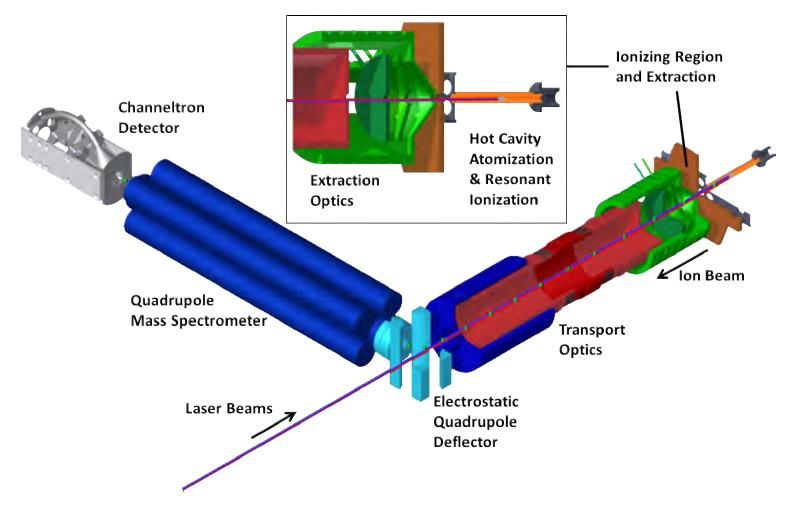
Table of Contents
1. Objectives ........................................................................................................................................ 3
2. Theoretical background................................................................................................................... 3
 2.1 Resonance ionization spectroscopy .............................................................................................. 3
 2.1.1 Non-resonant ionization......................................................................................................... 4
 2.1.2 Autoionization ........................................................................................................................ 4
 2.1.3 Ionization via Rydberg states ................................................................................................. 4
 2.2 Spectroscopy of Ytterbium ............................................................................................................ 5
3. Experimental setup ......................................................................................................................... 5
 3.1 MABU – Mainz Atomic Beam Unit ................................................................................................ 5
 3.1.1 Ion source ............................................................................................................................... 6
 3.1.2 Extraction and Ion Optics ....................................................................................................... 6
 3.1.3 Quadrupole mass spectrometer (QMS) ................................................................................. 6
 3.1.4 Ion counter ............................................................................................................................. 6
 3.2 The Titanium:Sapphire Laser system............................................................................................. 7
 3.2.1 Grating-Laser .......................................................................................................................... 7
 3.2.2 Laser Scan ............................................................................................................................... 8
4. Experimental tasks ........................................................................................................................ 11
 4.1 Task 1 – Obtain the ion signal...................................................................................................... 11
 4.2 Task 2 – Mass scan ...................................................................................................................... 14
 4.3 Task 3 - Line profile and laser power dependence of the first excitation step ........................... 14
 4.4 Task 4 - Broad-band laser scan of the second excitation step .................................................... 16

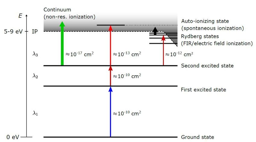
1. Objectives
The goal of this experiment is to get basic knowledge/experience in the field of resonance ionization
spectroscopy. The measurements will be performed on ytterbium (Yb), which is a lanthanide with a relatively
simple and well-known spectrum. This element has multiple isotopes, which can be nicely seen in a mass
spectrum. For an overview of the isotope ratios, the corresponding section of the Karlsruhe Nuclide Chart is
shown in Figure 1. The following spectroscopy will be conducted on the most abundant stable isotope - 174Yb.
Moreover, Yb is iso-electronic to nobelium - one of the actinides, which are the objectives of the LISA project.

 Figure 1 - Section of the Karlsruhe Nuclide Chart, showing the stable isotopes of ytterbium.

2. Theoretical background
 2.1 Resonance ionization spectroscopy
Laser resonance ionization was first proposed as a selective spectroscopy method by T. Ambartzumian and V.
Letokhov in 1972 [1]. Since then, this method has been widely used and can be found at many accelerator
facilities nowadays, mainly in the form of laser ion sources [2]. The laser resonance ionization method is based
on the stepwise resonant excitation of atoms from the ground state to beyond the first ionization potential. In
this process, typically one to two intermediate levels are populated using transitions as strong as possible. This
process is illustrated in Figure 2. The ionization process occurs from the intermediate level that is energetically
highest. There are three basic ways to ionize: non-resonant photoionization, excitation of autoionizing states, or
ionization via Rydberg states. The ionized atom is transported via electric fields of ion optics from the ionization
region to a detector.

Figure 2 - Schematic description of Resonance Ionization Spectroscopy. The arrows indicate the step-wise optical excitation from the atomic
ground state to ionization. The ionization efficiency crucially depends on the final excitation step, which may address the continuum, Rydberg-
states or autoionizing states. The lowered IP on the right indicates an electric field, which effectively reduces the ionization threshold.
Approximate excitation cross sections are given. For details see text [3].

The position of the individual energy levels is characteristic for each element. This is referred to as an atomic
fingerprint. Due to the uniqueness of the excitation spectra, laser resonance ionization is a highly element-
selective method. Typical ionization potentials are around 5-7 eV for the lanthanides. These energies can be
achieved with two or three photons from the visible and ultraviolet regions. (Photons with wavelengths in the
visible range (400 – 800 nm) have energies between 1.5 and 3 eV). The combination of several resonant
transitions increases the selectivity of the ionization process. Usually, laser ionization is combined with mass
separation to be able to get isotopically pure ion beams. This combined process is often referred to as resonance

ionization mass spectrometry (RIMS). The mass selection can be carried out either with the aid of a RF
quadrupole, a time-of-flight spectrometer (ToF), or an electromagnet. The RIMS method is of high relevance for
the production of isotopically pure radioactive ion beams. For spectroscopic studies, the ion signal is recorded as
a function of the wavelength of an excitation step.

 2.1.1 Non-resonant ionization
Non-resonant ionization is generally much less efficient than the resonant processes of AI or Rydberg excitation.
The frequency of the final excitation step laser only has to be high enough to excite one electron beyond the
ionization threshold. Typical cross-sections for this process are in the range of ≈ 10−17 cm2 [4]. A non-
resonant ionization step is used when a new lower resonant excitation step is to be found. Despite the relatively
low efficiency, non-resonant ionization offers the advantage of simplicity (no precise wavelength tuning, no
selection rules). Furthermore, non-resonant ionization may be advantageous for spectroscopy of the hyperfine
structure. This ensures that the hyperfine structure splitting of a resonant ionization step does not overlap the
structure to be investigated.

 2.1.2 Autoionization
An autoionizing state (AIS) is a multi-electron excitation with an energy greater than the ionization potential. Due
to the wave function overlap, there is a high probability that the total energy is transferred to one electron, which
is then ejected from the atom. The theory of autoionizing processes was provided by Ugo Fano [5]. There, by
means of perturbation calculation, the effective cross-section of such a process is derived to [6]
 2
 Γ
 ( + − 0 )
 = 2
 Γ2
 ( − 0 )2 +
 2
with the shape parameter q, the linewidth Γ, the energetic position of the resonance E 0, and the total energy
supplied ε. This equation is called Fano profile and serves as a fitting function for autoionizing states to determine
the position of resonance E0 in the energy spectrum. When such a state is resonantly excited, effective cross-
sections of σAI ≈ 1015 cm2 are achieved [7], which is why this ionization mechanism is the most efficient of those
listed here. Since the lifetime of a AIS is typically very small, auto-ionizing transitions have linewidths, which can
be up to many orders of magnitude larger than transitions between bound states [7]. Ionization via autoionizing
states is generally used in applications that require a high ionization efficiency.

 2.1.3 Ionization via Rydberg states
Another form of resonant ionization is the ionization over Rydberg states. These states are just below the
ionization potential, so only little energy is needed for ionization. Typically, the binding energies for observable
Rydberg states in our apparatus are between 3 meV and 200 meV, i.e. 240 cm-1 to 1600 cm-1. The necessary
energy for ionization can be provided by different mechanisms: photons from any incident laser, blackbody
radiation in the hot ion source, electric fields, or collisions (Rydberg atoms have huge collisional cross-sections).
The atoms excited into a Rydberg state are also called Rydberg atoms. One electron is excited to a high principal
quantum numbers and accordingly the atomic radius can be several micrometers large. Due to the large orbit of
the excited electron far away from the atomic core, this quantum mechanical problem is similar to that of the
hydrogen atom. The shielding of the atomic core by the inner electrons is especially large for high angular
momentum quantum numbers, and is described by the quantum defect δ(n,l). The energy levels are described
by the so-called Rydberg-Ritz formula:
 
 = − = −
 ( ∗ )2 ( − ( , ))2

with the effective quantum number n and the ionization potential E IP. For high principal quantum numbers, the
quantum defect converges to a fixed value, which depends only on l. The quantum defect can be expressed as
the series

 ( , ) = + + +⋯
 ( − )2 ( − )4

where the parameters A, B, C are to be determined based on the data. For an analysis of the Rydberg series and
for the determination of the ionization potential the first terms of the development are sufficient.

The maximum cross-section σRyd(n) as a function of the principal quantum number n for the ionization is [7]
 64 
 ( ) = 02 ≈ ∙ 10−17 cm2
 3√3

with the fine structure constant α and Bohr radius a0.

 2.2 Spectroscopy of Ytterbium
Ytterbium is the second last element in the lanthanide series, where the 4f shell is completely filled with 14
electrons. Furthermore, since the 6s shell is terminated and the 5d shell is unoccupied, Yb has no free electrons
in the ground state. The ground state configuration of Yb I is [Xe] 4f 146s2. The excitations scheme to be used in
this experiment is shown in Figure 3.

 Figure 3 - Illustration of the excitation scheme of ytterbium. The required laser wavelength is in the UV range [8].

3. Experimental setup
 3.1 MABU – Mainz Atomic Beam Unit
The Mainz Atomic Beam Unit (MABU), is a compact RIS setup, which was built up in the framework of the
dissertation of Sebastian Reader [9]. In subsequent work, the apparatus has been further modified and
continuously improved [10], [11]. Many elements have been studied using MABU. Regarding the actinides, the
IP of Ac [12], hyperfine structures of ground-state transitions in Th [13], more than 2000 resonances of Pa [14],
the isotope shifts of Pu [15], and many more have been measured. Figure 4 shows a computer drawing of the
MABU. The most important components are briefly explained below.

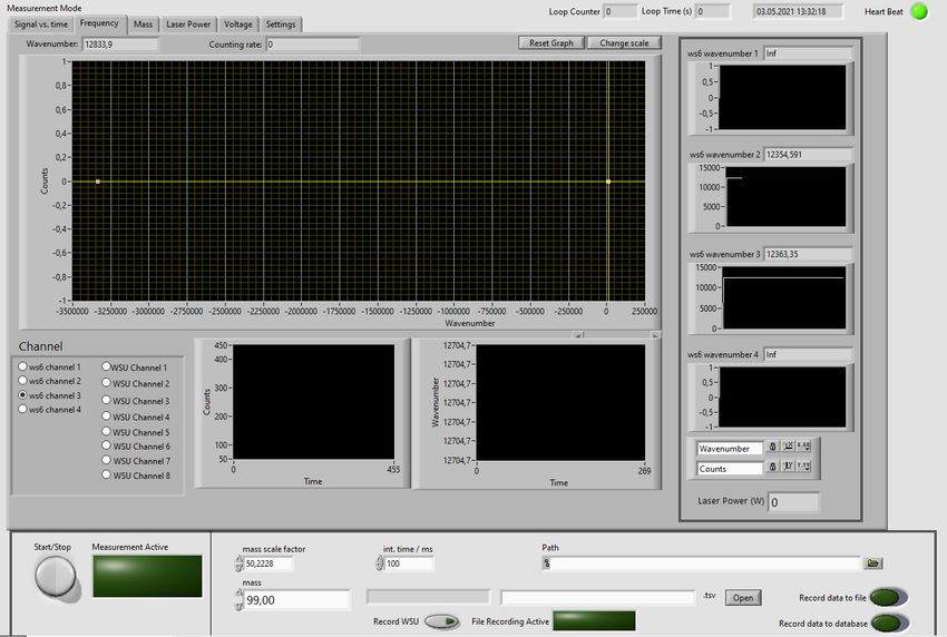
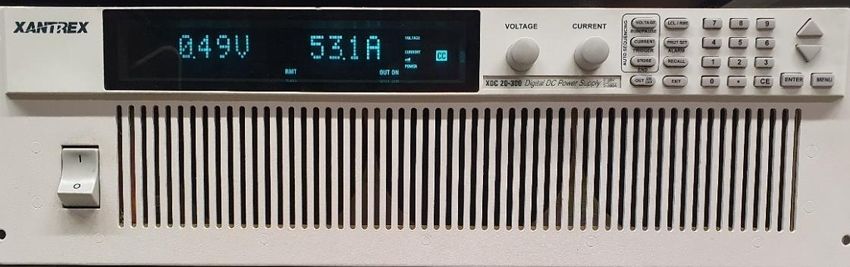
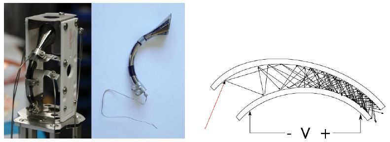
Figure 4 - CAD-drawing of the main components of the MABU with a magnified representation of the source region as inlay [11].

 3.1.1 Ion source
The ion source consists of a resistively heated tantalum tube with a length of 3.5 cm and an inner diameter of
2.2 mm into which the sample material is placed. The sample is usually prepared on a support foil made of
tantalum, zirconium, or hafnium, which also serves as a reduction material during atomization. The source can
be heated to a temperature of about 2000°C, with a maximum heating current of 300 A. To protect the
surrounding components from the high temperatures and to reduce the required heating power, a heat shield
surrounds the source. Several water-cooled copper rods serve as both support and current feedthrough. At a
sufficiently high temperature, atomic gas is formed inside the tantalum tube. The laser beams are collinearly
superimposed into this gas for ionization. Alternatively, it is possible to ionize the atoms leaving the source with
laser beams transversely superimposed in front of the outlet opening. In this way, a reduction of the Doppler
width and thus a higher resolution can be achieved [16].

 3.1.2 Extraction and Ion Optics
The generated ions are first accelerated by three extraction electrodes and formed into a beam. Subsequently,
the ion beam is focused by an electrostatic einzel lens. It consists of a triple tube lens, which is shown in red in
Figure 4. An additional tube lens after the einzel lens can act as a telescope to influence the size and focus of the
ion beam. A subsequent quadrupole deflector guides the beam to the quadrupole mass spectrometer and is used
to separate the ions from the neutral particles. In addition, this geometry allows easy injection of the laser. The
voltages of the individual ion optical elements can be adjusted during an experiment to optimize the signal.
Detailed information about ion optics in general can be found in [17].

 3.1.3 Quadrupole mass spectrometer (QMS)
The RF quadrupole filters ions according to their mass to charge ratio. For singly charged ions, as obtained by
RIS, only ions of a chosen mass are transmitted to the detector. Details are subject of the mass filter lab course.

 3.1.4 Ion counter
After passing the quadrupole mass filter, the remaining ions are detected. Especially for small sample it is
important to be able to detect individual ions with high efficiency. In this experiment a channel electron
multiplier - channeltron is used. Such a detector is shown in Figure 5. It belongs to the class of (continuous)
secondary electron multipliers. A channeltron is a bent tube made of insulating material, on the inside of which
a high-resistance layer is applied. A voltage of few kV is applied between the funnel-shaped opening and the end

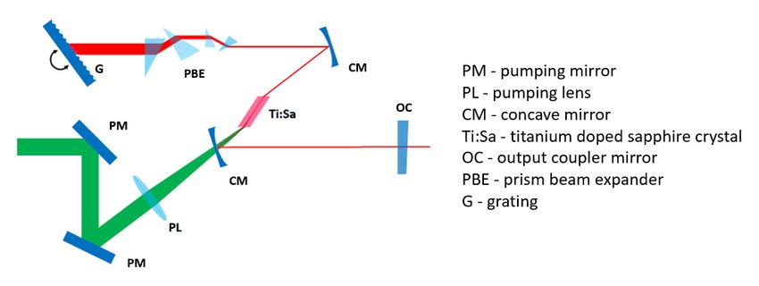
of the tube. This generates an electric field along the tube axis. When a particle hits the surface of the entrance
region, it releases several secondary electrons, which are again accelerated, leading to an electron avalanche and
a detectable signal at the end contact. This principle is illustrated in Figure 5 on the left side. An amplifier, a
discriminator, and an analog-to-digital converter can be used to register and store a counter signal. Channeltron
electron multipliers are characterized by very high detection efficiency and low dark count rates at low count
rates. The efficiency can be estimated at almost one, the dark count rate is below 0.1 events per second.

Figure 5 – The detector used is a channel electron multiplier, which can be seen in the right pictures in the installed and removed states. The
operation of the secondary electron multiplier is shown schematically in the left figure [10].

 3.2 The Titanium:Sapphire Laser system
The laser system used in this experiment consists of a commercial pulsed Nd:YAG pump laser and
Titanium:Sapphire Lasers developed in the group in the course of different thesis projects. These lasers are
characterized by high output power and a wide tuning range, allowing resonant excitation of atomic transitions
for a large fraction of all elements. The lasers developed in Mainz are used at many different research institutions.
In the following, the grating-based laser will be presented.

 3.2.1 Grating-Laser
The Mainz Titanium:Sapphire Grating-Laser is based on a Z-shaped resonator (Figure 6). The Ti:sa crystal is
pumped by a pulsed pump laser at 10 kHz repetition rate with 150 ns pulses. The pump power is usually around
12 W. The maximum achievable output power of the Ti:sa laser is about 2.5 W and the linewidth is between 1
GHz and 2.5 GHz. The tuning range extends from about 700 nm to just above 1000 nm. The laser was developed
as part of Christoph Mattolat's dissertation [18] and improved and characterized in detail by Pascal Naubereit in
his master's thesis [19].

Figure 6- Schematic structure of the grating laser. The end mirror is replaced by a rotatable reflection grating and provides the frequency
selection via the set angle. The prism beam expander (PBE) enlarges the beam radius in front of the grating. Figure adapted from [14].

The frequency selection is achieved by a tunable Littrow grating. The principle is shown in Figure 7.

Figure 7- Left: Schematic representation of the principle of a reflection grating. The incident beam strikes the grating normal at an α angle
and is reflected at an β angle. The path differences can be calculated via the groove spacing d. Right: Littrow configuration. The angle of
incidence α equals the reflection angle β. Constructive interference can be optimized for certain wavelengths with so-called blaze angle ΘB.
[3].

In zeroth order the beam is reflected on the ‘’superstrate’’ (the groove envelope) with respect to the grating
normal α = α’. Higher diffraction orders, on the other hand, follow a wavelength-dependent pattern. From the
path difference between the two partial waves follows the grating equation

 d (sin(α) + sin(β)) = mλ,

where in the Littrow configuration α = β applies. The first refraction order beam is then reflected into itself. Thus,
the grating acts as a wavelength-selective mirror, and by changing the angle of incidence (by rotating the grating)
the frequency of the laser can be tuned. The groove slope is characterized by the blaze angle θB. The right choice
of θB leads to optimal first order diffraction for a given wavelength λB. In our experiment we use a blazed grating
at λB = 800 nm. The resolving power of a reflection grating results from the number of illuminated grooves N and
the interference order m according to

 = .
 Δ 
Therefore, the laser beam is expanded by an array of multiple prisms in front of the grating.

 3.2.2 Laser Scan
The wavelength change of the Grating-Lasers has been automatized. The grating and BBO position
can be control by the computer in order to easily perform broad scans. Below are the instructions for
both lasers used in the experiment.

1. First laser (Grating 2)
The wavelength of the first laser can be changed by the GratingControl-driver2.vi (Figure 8), where the position
of the grating can be changed (Do not apply steps larger than 0.01!). Big change should be followed by the
change of the BBO crystal position to keep the maximum laser power. This has to be done manually.

2. Second laser (Grating 1)
The wavelength of the second laser can be modified by Scanner.vi (Figure 9) in two ways:

1. Manually. The wavenumber can be changed in the box ‘’Grating Pos. Setpoint’’ (Do not apply steps
 larger than 0.01!). This should be followed by the change of the BBO crystal position to keep the
 maximum laser power. The BBO position can be changed in the box ‘’Piezo Pos. Setpoint’’ (Piezo controls
 the position of the BBO. Do not apply steps larger than 0.01!). The relative power of the laser is shown
 in the left top plot as a function of Piezo position.

2. Automatically.
 In the tab ‘’PID-Control’’:
 1. Set ‘’Power Setp’’ (around 200 mW less than max. relative power).
 2. Set ‘’min. Power’’ (~ 800 mW).
 3. Press ‘’Neu initialisieren”.
 In the tab ‘’Control’’:
 1. Set ‘’Zielwert’’ to -5 to scan UP or to 5 to scan DOWN.
 2. Set ‘’Stepwidth ‘’:
 a. FAST scan 0,001
 b. SLOW scan 0,0001
 3. Change ‘‘Piezo Pos. Setpoint”:
 a. Scan UP - Go to the LEFT side of the max. power.
 b. Scan DOWN - Go to the RIGHT side of the max. power.
 c. Do not apply steps larger than 0.01!
 d. See the left plot in Figure 9.
 4. Press ‘’Scan’’.

 Figure 8- GratingControl-driver2.vi - program controlling the grating position of the first laser.

-5 5
scan up scan down

 Figure 9- Scanner.vi - program enabling scan of the second laser.

 Figure 10 - Scanner.vi - program enabling scanning of the second laser. Power Setup for automatic scan.

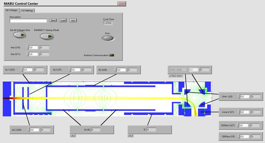
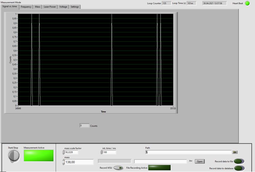
4. Experimental tasks
The goal of this experiment is to get the basic knowledge about resonance laser spectroscopy. In order to do it,
you will have to perform a few tasks:

 1. Turn on the apparatus and obtain the ion signal to be able to perform the following tasks. To do
 so you will have to:
 a. optimize the lasers,
 b. optimize the ion optics,
 c. heat the source.
 2. Mass scan to check the composition of the sample. You have to:
 a. record a mass scan,
 b. determine isotopes ratio.
 3. Line profile and laser power dependence of the first excitation step:
 a. record the ion signal as a function of the laser power,
 b. record the spectral line profile for different laser powers.
 4. Broad-band laser scan of the second excitation step.

The QMS, lasers, and power supplies will be switched on ahead before the experiment.

 4.1 Task 1 – Obtain the ion signal
a. Optimize the lasers

 Set up the lasers according to the scheme in Figure 3.

How to change the wavelength of the lasers you can find in subsection 3.2.2 Lase Scan.

b. Optimize the ion optics

The ion optics of MABU is controlled from the computer by the Ion Optics Control.vi (Figure 11), where you can
see the cross-section of MABU and respective electrodes. In order to transport ions from the ion source (left side
of Figure 11) to the QMS, the voltages have to be tuned for optimal transmission. To see the influence of the
certain electrode you can play a bit with the voltages by simply introducing the desired voltage into a white box
close to the name of the electrode. Some of the electrodes have only grey boxes, which means that you cannot
change them. For example, the relation AL3 = RL1 = RL3 = TL is implemented to keep the beam at the same
energy. From the working principles of the deflector, the average of opposite electrodes - UML- and UML+ should
be at the potential of the beam, therefore UML- is equal to 2AL3 - UML+.

The influence of the ion optics can be seen in the signal from the detector in the MABU.vi - Figure 12. In the first
tap of this program – ‘’Signal vs. time’’ you can see counts over time. From this tab you can also control, the mass
of ions which should be transmitted through the quadrupole. By pressing the ‘’Start/Stop’’ button you can start
and stop the measurement.

 Apply voltages to the electrodes to be able to see the signal, when the ions will be created.

Figure 11- Ion Optics Control.vi - ion optics control panel. See more in the text.

Figure 12- MABU.vi - MABU “Signal vs. time” control panel. See more in text.

c. Heat the source

The heating of the source is controlled by the Xantrex300A.vi presented in Figure 14. This program controls the
XDC 20-300 Digital DC Power Supply - Figure 13, which provides the current through the source.

 Figure 13- XDC 20-300 Digital DC Power Supply by which the source is heated.

In the box ‘’Line Setpoint Current’’ you set the current which goes through the source to heat the sample. The
box ‘’Line Ramp Time’’ indicates the time which should take to increase the current. The introduced values you
can apply by pressing ‘’ > ’’. If the heating time is too short, the program will not allow these settings, and the
square indicator on the right side of the ‘’ > ’’ will glow red. In this case you should choose a longer ramp duration.
You can heat quickly to around 80 A and then slowly heat the source looking at the signal from the detector.

When you see some signal, you should check the adjustment of the lasers (not only the wavelengths but also
the position at which they enter MABU) and the optimization of the ion optics then you can heat more. Your
goal is to obtain around a few hundred counts.

 Figure 14- Xantrex300A.vi - Ion source control panel. See more in text.

 Heat the source.

 Find the signal.

 Reoptimize lasers and ion optics.

 How can you verify that the ion signal is Yb?

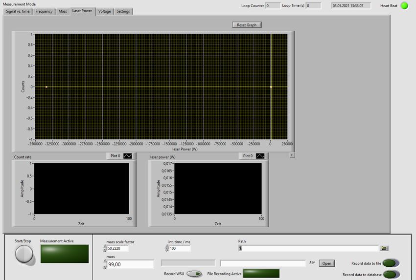
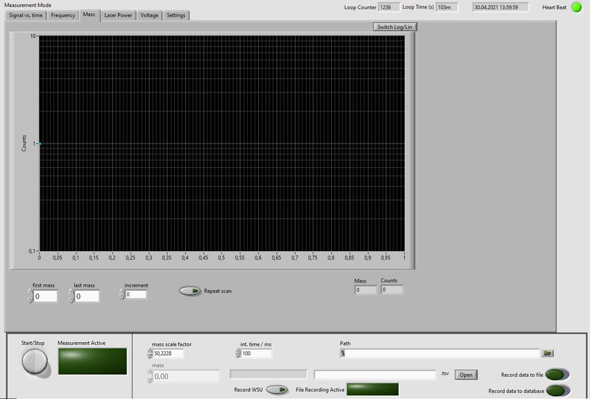
4.2 Task 2 – Mass scan
a. Record a mass scan

Now when everything is optimized you can check the composition of your sample. This can be done in the same
program, which you use to measure the counts, you should stop the measurement and then change the tab to
‘’Mass’’. There, in boxes ‘’first mass’’ and ‘’last mass’’ you can introduce the range of the masses you want to
scan. In the field ‘’increment’’ you should put the step of the scan.

Figure 15- MABU.vi - MABU ”Mass” control panel. See more in text.

 Perform a mass scan, think about the mass range and the step of the scan.

b. Determine isotope ratio

 Is it in the agreement to the natural isotope ratio?

 How can the laser influence the isotope ratio?

 4.3 Task 3 - Line profile and laser power dependence of the first excitation step
a. Record the ion signal as a function of the laser power

The saturation power of the transition can be determined by measuring the ion signal as a function of laser
power. The saturation power indicated the laser power needed to reach 50% of the maximum transition rate on
the corresponding transition. In order to see the saturation behavior of the first excitation step, you have to
measure the ion signal as a function of laser power. Set the laser at FES – 1234.11 cm-1 and go to the tab – ‘’Laser

power’’ in MABU.vi (Figure 16). To send the value of the power from the power meter to the PC the PM100D.vi
has to run.

 Figure 16- MABU.vi - MABU “Laser Power” control panel. See more in text.

Due to the large transition strengths in the first excitation step, saturation is already expected here at low
powers.

 Where is the power meter placed?

 How much power of the beam does it measure?

 How can you control the laser power?

 Record the ion signal as a function of laser power.

 What is the saturation power?

b. Record the spectral line profile for different laser powers

Record the spectral line profiles by varying the frequency of the laser for the first step.

The signal can be recorded in the tab ‘’Frequency’’ of the MABU.vi, where you have to choose the correct channel
of the wavelength meter - Figure 17.

Figure 17- MABU.vi - MABU “Frequency” control panel. See more in text.

 How does the laser power influence the line profile?

 What is the spectral linewidth?

 Does it correspond to the natural linewidth?

 4.4 Task 4 - Broad-band laser scan of the second excitation step
To perform the scan, you have to go to tap ‘’Frequency’’ in MABU.vi, where you can display the counts over the
wavelength of the scanning laser - Figure 17. The scan of the laser can be performed automatically by the
Scanner.vi (Figure 9) (see 3.2.2).

 At which wavenumber do you expect IP?

 How can we determine the IP from the spectrum of the second excitation step?

 What transition do you expect below the ionization potential?

 What are their electron configurations?

 How can the polarization of the laser influence the transition strength?

Bibliography

 [1] T. Ambartzumian and V. Letokhov, "Selective Two-Step (STS) Photoionization of Atoms and
 Photodissociation of Molecules by Laser Radiation," Appl. Opt, vol. 11, pp. 320-331, 1972.

 [2] B. Cheal and K. Flanagan , "Progress in laser spectroscopy at radioactive ion beam facilities,"
 Journal of Physics, vol. 11, pp. 320-331, 1972.

 [3] D. Studer, Probing atomic and nuclear structure properties of promethium by laser
 spectroscopy, Dissertation, Johannes Gutenberg-Universitat Mainz, 2020.

 [4] W. Demtroder, "Laserspektroskopie 2," Springer Verlag, no. 978-3-642-21446-2, 2013.

 [5] U. Fano, "Effects of configuration interaction on intensities and phase shifts," Phys. Rev., vol.
 124, no. 6, pp. 1866-1878, 1961.

 [6] A. Hakimi, Diodenlaserbasierte Resonanzionisations-Massenspektrometrie zur Spektroskopie
 und Ultraspurenanalyse an Uranisotopen, Dissertation, Johannes Gutenberg-Universitat, Mainz,
 2013.

 [7] T. Kessler, Development and application of laser technologies at radioactive ion beam facilities,
 Dissertation, University of Jyvaskyla, 2008.

 [8] "RILIS Elements," [Online]. Available: https://riliselements.web.cern.ch/index.php.

 [9] S. Raeder, Spurenanalyse von Akitniden in der Umwelt mittels Resonanzionisations-
 Massenspektrometrie, Dissertation. Mainz: Johannes Gutenberg-Universitat , 2010.

 [10] J. Rossnagel, Aufbau einer Atomstrahl-Massenspektrometer-Apparatur zur resonanten
 Laserionisation, Diplomarbeit. Mainz: Johannes Gutenberg-Universitat, 2011.

 [11] M. Franzmann, Resonanzionisationsmsssenspektrometrie an Aktiniden mit der Mainzer
 Atomstrahlquelle MABU, Diplomarbeit. Mainz: Johannes Gutenberg-Universitat, 2013.

 [12] J. Rossnagel and e. a. Raeder, "Determination of the first ionization potential of actinium," Phys.
 Rev., vol. 85, 2012.

 [13] V. Sonnenschein, S. Raeder and e. al., "Determination of the ground-state hyperfine structure
 in neutral Th-229," J. Phys. B, vol. 45, p. 165005 – 165005, 2012.

 [14] P. Naubereit, T. Gottwald and e. al., "Excited atomic energy levels in protactinium by resonance
 ionization spectroscopy," Phys. Rev. A. , vol. 98, 2018.

 [15] A. Voss, V. Sonnenschein and e. al., "High-resolution laser spectroscopy of long-lived plutonium
 isotopes," Phys. Rev. A., , vol. 95, p. 032506 –, 2017.

 [16] T. Kron, Pushing the Limits of Resonance Ionization Mass Spectrometry - Ionization Efficiency in
 Palladium and Spectral Resolution in Technetium, Mainz: Johannes Gutenberg-Universitat,
 2016.

[17] H. Liebl, Applied Charged Particle Optics, Springer-Verlag Berlin Heidelberg, 2008.

[18] C. Mattolat, Spektroskopische Untersuchungen an Technetium und Silizium, Dissertation at
 Johannes Gutenberg-Universitat in Mainz, 2010.

[19] P. Naubereut, Weiterentwicklung eines weitabstimmbaren Titan:Saphir-Lasers und sein Einsatz
 zur Spektroskopie hochliegender Resonanzen in Holmium, Masterarbeit. Mainz: Johannes
 Gutenberg-Universitat, 2014.

[20] A. Kramida, Y. Ralchenko, J. Reader and NIST ASD Team (2020), “NIST Atomic Spectra
 Database,” 30 March 2021. [Online]. Available: https://doi.org/10.18434/T4W30F.

[21] F. Weber, Effizienter elementselektiver Nachweis von Lanthaniden mit RIMS, Mainz:
 Masterarbeit in Physik vorgelegt dem Fachbereich Physik, Mathematik und Informatik der
 Johannes Gutenberg-Universitat Mainz, 2018.

[22] P. Wolfgang and H. Steinwedel, Notitzen: Ein neues Massenspektrometer ohne Magetfeld,
 Zeitschrift fur Naturforschung, 1953.

[23] E. Mathieu, "Memoire sur Le Mouvement Vibratoire d'une Membrane de forme Elliptique,"
 Journal de Mathematiques Pures et Appliquees, pp. 137-203, 1868.

[24] K. Blaum, Resonante Laserionisations-Massenspektroskopie an Gadolinium zur
 Isotopoenhaufigkeitsanalyse mit geringsten Mengen, Dissertation. Mainz:Johannes Gutenberg-
 Universitat, 2000.

[25] W. Paul, H. P. Reinhard and U. von Zahn, "Das elektrische Massenfilter als Massenspektrometer
 und Isotopentrenner," Zeitschrift fur Physik, no. 152.2, pp. 143-182, 1958.