Optimization of a Centrifugal Compressor Using the Design of Experiment Technique - MDPI
←
→
Page content transcription
If your browser does not render page correctly, please read the page content below
applied
           sciences
Article
Optimization of a Centrifugal Compressor Using
the Design of Experiment Technique
Mohammad Mojaddam 1, *,†               and Keith R. Pullen 2, *
 1    Mechanical Engineering and Energy Department, Shahid Beheshti University, Tehran 167651719, Iran
 2    School of Mathematics, Computer Science and Engineering, University of London, London EC1V 0HB, UK
 *    Correspondence: m_mojaddam@sbu.ac.ir (M.M.); k.pullen@city.ac.uk (K.R.P.); Tel.: +98-21-7393-2681 (K.R.P.)
 †    Current address: Shahid Beheshti University, Tehran 167651719, Iran

 Received: 24 November 2018; Accepted: 8 January 2019; Published: 15 January 2019

 Abstract: Centrifugal compressor performance is affected by many parameters, optimization of which
 can lead to superior designs. Recognizing the most important parameters affecting performance helps
 to reduce the optimization process cost. Of the compressor components, the impeller plays the most
 important role in compressor performance, hence the design parameters affecting this component
 were considered. A turbocharger centrifugal compressor with vaneless diffuser was studied and
 the parameters investigated included meridional geometry, rotor blade angle distribution and start
 location of the main blades and splitters. The diffuser shape was captured as part of the meridional
 geometry. Applying a novel approach to the problem, full factorial analysis was used to investigate
 the most effective parameters. The Response Surface Method was then implemented to construct
 the surrogate models and to recognize the best points over a design space created as based on the
 Box-Behnken methodology. The results highlighted the factors that affected impeller performance
 the most. Using the Design of Experiment technique, the model which optimized both efficiency and
 pressure ratio simultaneously delivered a design with 3% and 11% improvement in each respectively
 in comparison to the initial impeller at the design point. Importantly, this was not at the expense of
 sacrificing range, of critical concern in compressor design.

 Keywords: centrifugal compressor; Design of Experiment (DoE); full factorial analysis; Box-Behnken
 design; response surface method

1. Introduction
      Design and optimization of rotating machines by means of the numerical optimization methods
has become an established technique in all industries for many decades.
      In centrifugal compressors, the impeller plays a most important role in machine performance and
this has attracted significant interest of researchers’ and developers over several decades. Not only will
a good impeller design bring significant performance benefits itself, but a good impeller will deliver a
more uniform flow to the diffuser hence improving the performance of the whole compressor.
      In the preliminary design stage, inlet and outlet angles and the main dimensions of the impeller
are obtained. This design will be followed by detail design where the complete gas path and the
geometry are specified which includes hub and shroud contours and the blade curvature for the vaned
components [1]. During detail design some adjustments are repeatedly necessary as the acceptable
performance in a relatively wide design range is constrained by some limitations [2]. Thermodynamics
and fluid mechanic principles, mechanical, vibration, and the manufacturing constraints and the
cost dictate these limitations. Design and optimization of rotating parts by means of the numerical
optimization methods has become an established technique for recent decades. Numerical optimization

Appl. Sci. 2019, 9, 291; doi:10.3390/app9020291                                   www.mdpi.com/journal/applsci
Appl. Sci. 2019, 9, 291                                                                           2 of 19

techniques help compressor designers obtain optimum efficiency or maximum pressure ratio [3] or
widener stable operating range [4].
     Evaluating the effect of different aspects in the optimization process simultaneously imposes
heavy computational cost, hence some techniques are developed to reduce the problem exploring
space. The Design of Experiment (DoE) technique is one of this methods. The DoE technique helps the
designer limit the calculations needed to find the effects of input variables on the output variables.
In this technique the shortcoming of inaccuracy of using an approximation function is compensated by
reducing the number of calculations. A combination of mathematical and statistical methods are used
for constructing the design space [5].
     Many researchers have targeted the optimization of centrifugal compressors. Many parameters
are considered in this regard. For example optimization techniques were implemented to optimize
the blade profile [6], meridional profiles [7,8], blade sweep angle [9], the splitter [10], the vaneless
diffuser [11] and there are many others.
     In the metamodeling technique to build a surrogate model, DoE can be employed to generate
appropriate training samples [12]. Barsi et al. optimized the geometry of a return channel for a
centrifugal compressor through the artificial neural network (ANN) method which is trained using
a database of 3D CFD solutions created with a DoE technique [13]. Kim et al. also optimized the
meridional geometry of an impeller. They used Latin-hypercube sampling of DoE to generate design
points for implementing the Neural Network (NN) method [14].
     Siemann and Seume designed a compressor diffuser using DoE to see the effects of four parameters
and their interactions on the blade efficiency [15].
     Bonaiuti et al. presented a parametric study for an optimization problem using DoE. They
identified the most influential geometrical factors affecting impeller performance and optimized three
different impellers [16]. Guo et al. optimized a centrifugal compressor impeller using DoE and
response surface models to increase pressure ratio, isentropic efficiency and to reduce work input of a
compressor [17].
     Tang et al. introduced a response surface method for constructing a surrogate model to
parametrize the design space for aerodynamic optimization of a transonic fan [18]. Wang et al.
considered the β angle distribution to optimize a centrifugal compressor impeller. They implemented
the Kriging interpolation to construct the approximation function [19].
     In this article three main characteristics of an impeller are considered for investigation of their
effects on performance. The meridional contour geometries, the angle distribution of the blades and
the leading edge of main blades and splitters are parametrized in this regard. Parameterization of
the meridional geometry also defines the vaneless diffuser including the level of pinch, vital ensure
capture of the full compressor geometry. The Full Factorial method is used in each step to explore the
most influential factors. The models are created and solved by implementing a three dimensional
viscous solver and the CFD outputs are used to obtain each model performance including the pressure
ratio and isentropic efficiency. The Box-Behnken method is used to construct the design space for the
selected parameters. Second-order polynomial regression is used to construct the response surface for
optimizing pressure ratio and efficiency simultaneously.

2. Bézier Curve
    Bézier curves are selected for describing the geometry of curves. A Bézier curve of degree n is a
polynomial curve which is expressed in the following form,
                                          n
                                p(t) =   ∑ ci Bin (t)          t ∈ [0, 1]                            (1)
                                         i =0

in which, the ci are the control points and Bin is ith Bernstein polynomial of degree n, by
following definition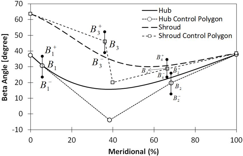
Appl. Sci. 2019, 9, 291                                                                               3 of 19


                                                    n i
                                       Bin (t)   =     t (1 − t ) n −i     i ∈ [0, n]                    (2)
                                                    i
     Bézier curves allow control of the curves systematically and the derived curve is smooth with
continuous derivatives [2]. The lines between consecutive control points are named the control polygon.
The Bézier curve passes through only the first and the last control points and tangent to the control
polygon at both ends. The most influential points are the end points and the middle control points
have lower weight in creating the curve and can be used for modification the curve. Figure 1 shows
the effect of changing a control point on a Bézier curve.

                          Figure 1. Bézier curve and the effect of control point position change.

3. Design of Experiment

3.1. Design Space
     To investigate the effect of each factor on the objective function, the full factorial design technique
can be used. A 2k full factorial design space is built by k parameters each at two levels results in 2k
design points. This type of design is helpful in early stages of design to recognize the most effective
parameters in the results.
     In the case with A, B, C and D as the factors, each at two levels, 24 combinations are generated.
Four of them are the main effects shown by A, B, C and D estimate the main effects of the related
factors on the the result. In six of them, the two factor interactions considered are shown by AB, AC,
AD, BC, BD and DC. The three parameters interactions are ABC, ABD, ACD and BCD. The four factor
interaction for this case is ABCD. The main effect of A, is the average of the results, in which the
combinations with A at the high level are positive ones and the combinations with A at the low level
are negative ones. For each parameter two levels are shown by + or − respectively. If the average
response at the combinations in which X at the high level is noted by y x+ and the average response
with X at the low level is noted by y x− , The effect of X combination on the objective function [5] will be,

                                                      EX = y x + − y x −                                 (3)

      To recognize the significant factors, a normal or half-normal probability plot analysis is the
simplest tool. Normal probability plots show that whether sample data conform a normal distribution
or not [5].
      For constructing a normal plot, the effects are first ranked from smallest to largest, E1 < E2 <
... < En , Then the ordered Ei are plotted versus:

                                                         100(i − 0.5)
                                                                                                         (4)
                                                              n
Appl. Sci. 2019, 9, 291                                                                                  4 of 19

      Then a straight line interpolated between the 25th and 75th percentile points. The factors that have
negligible effect on the objective function have normally distributed Es and they fall along a straight
line, whereas most effective factors are far from the straight line and hence normal distribution [5].

3.2. Box-Behnken Technique
     Different types of designs are being used for creating the design space. The Full Factorial
Technique is a useful technique for exploring all of the design space. With n parameters, each at k level,
the full factorial creates kn design points. Two-level factorial techniques are very efficient but they
result in first-order models and cannot detect curvature. At Three-level, the 3n factorial, is not efficient
and generates huge design space points [20].
     Box-Behnken is a technique which makes an efficient design space and it requires only the fraction
of full factorial points to estimate the second-order effects of the response surface. For A, B and C
factors each at three levels {−1, 0, 1}, Box-Behnken design offers the points as shown in Figure 2 which
can be compared with 27 design points obtained from the full factorial technique.

                          Figure 2. Box-Behnken design space for three factors [20].

3.3. Response Surface Model
     After building the design space for each combination, the response (objective function) could
be derived. The response surface is constructed as a surrogate model based on the most important
effects. For instance if X,Y and XZ combinations show the largest effects on the objective function,
the estimated response surface [21] is defined as follows,

                                       yb = β 0 + β x X + β y Y + β xz XZ                                   (5)

in which β 0 is the average of the response for all combinations, β x is the EX /2 and so on. In this
relation the X,Y and XZ factors are varied in [−1, +1] intervals which correspond to variations between
low and high levels.
      To find the relationship between the objective function and factor values, the following
second-order polynomial model is used, in which { x1 , ..., xk } are the factors and β i s are the coefficients
and e is the approximation error.

                                          k          k
                              y = β 0 + ∑ β i xi + ∑ β ii xi2 + ∑ ∑ β ij xi x j + e                         (6)
                                        i =1        i =1          i< j

     The low order polynomial models may not be a reasonable approximation for entire design space;
however they work quite well over a relatively small part of the domain. The method of least squares
is used to estimate β coefficients in Equation (6). This method chooses β i s coefficients so that the sum
of the squares of the errors, L, is minimized.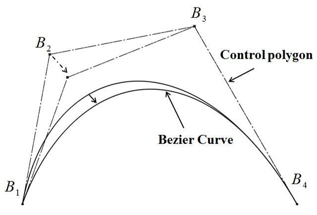
Appl. Sci. 2019, 9, 291 5 of 19
n n k 2
L= ∑ ei2 = ∑ yi − β 0 − ∑ β j xij (7)
i =1 i =1 j =1
3.4. Creating the Design Space
The parameters for the first three stages of the design space created are shown in Table 1. The
2k full factorial design technique is implemented in these stages for creating the design space. After
performing stage I to III the most effective parameters are recognized for the design space created in
stage IV.
Table 1. Stages I to III for recognizing the effective parameters.
Stage Concept Number of Factors Parameters
I Meridional Plane Geometry 5 M1 − M5
II Blade Angle Distribution 4 B1 − B4
III Blade Inlet Geometry and Splitter 4 I1 − I4
3.4.1. Stage I
Each parameter levels at stage I of the effective parameter recognition are shown in Figure 3.
A hub curve control polygon was constructed between two fixed points H1 and H2 and two control
parameters M1 and M2 . Fixed points and control points for constructing a Bézier curve for shroud
profile are S1 , S2 and M3 , M4 respectively. The diffuser inlet curve is also built on a fixed points F and
S2 and two control points are E and the a point along S2 M4 line (not shown in the Figure).
Figure 3. Parameters and their levels in Stage I.
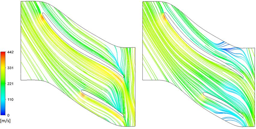
3.4.2. Stage II
The blade angle (angle β) distribution at hub and shroud is considered for parameter study in
this stage. The β angle is related to the azimuthal coordinate (angle θ) of blade curves through the
following relation [1].
rdθ
tan β = (8)
ds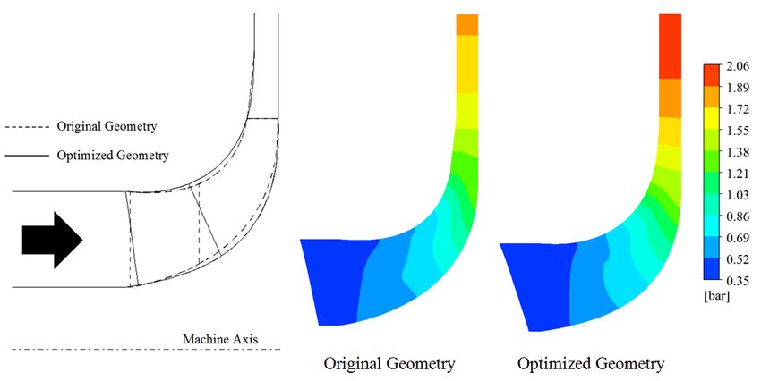
Appl. Sci. 2019, 9, 291                                                                            6 of 19

in which r is the radial coordinate and s is the meridional coordinate. A five control point Bézier curve
is fitted for each β angle distribution at hub and shroud (Figure 4). To build a domain space, the slope
of the control polygon at both ends are varied. The range of variation of the slopes is set to be at
maximum of 5 degrees from base case. Due to β distribution variation at hub and shroud, the blade
rake angle will change. The Blade Rake angle is the angle between the trailing edge and the tangential
direction at impeller tip. A rake angle up to 45◦ is commonly used [22] and the maximum value of
rake angle is kept constant (around 54.2◦ ) in this study.

                                    Figure 4. β angle distribution parametrization.

3.4.3. Stage III
     The leading edge of main blades and splitters are supposed to be changed in this stage. The main
geometry of meridional profile is held constant and the leading edge starting points, H1 and S1 , are the
lower limits for the leading edge. The upper limits for varying the position of H1 are toward the exit by
16% of hub curve length, and for the position of S1 are toward the exit by 10% of shroud curve length.
     The leading edge position of splitter can vary ±6.5% shroud profile length and ±7.5% hub profile
length related to their initial positions. Figure 5 shows the parameter bounds in this stage.

                          Figure 5. Main blade and splitter leading edge position parameters.
Appl. Sci. 2019, 9, 291 7 of 19
3.4.4. Stage IV
In this stage the Box-Behnken technique is used to create the design space based on the selected
parameters in the previous stages. An optimization process can take place in this stage regarding
meridional geometry, angle distribution and inlet geometry for blades simultaneously.
4. Geometry
A turbocharger compressor is modeled in this research. The compressor impeller has six main
blades and six splitters followed by a vaneless diffuser and an overhanging volute. The original
impeller and diffuser characteristics are tabulated in Table 2 and the cross section numbering is shown
in Figure 6.
The splitter leading edge starts at 47% hub and 29% shroud curve length from the inlet [23].
Through evaluating the effect of each parameter on the performance, all other parameters are
kept unchanged.
Table 2. Geometry characteristics.
Characteristics Values
Inlet Hub Radius(mm) 11
Inlet Shroud Radius(mm) 28
Impeller Axial Length(mm) 27.1
Discharge Radius(mm) 41
Discharge Width(mm) 5.7
Tip Clearance (mm) 0.4
Number of Blades 6
Number of Splitters 6
Diffuser Discharge Radius(mm) 72.25
Diffuser Outlet Width(mm) 4.27
Figure 6. Cross section numbering in meridional view.
5. Modeling
The aerodynamic model has been developed using ANSYS CFX 16.0. In this model, one passage
contains the inlet, impeller and diffuser and these are meshed using structured hexahedral grids.
O-type and H-type schemes are used for the leading edge and trailing edge of blades respectively.
The tip clearance is considered in the model and the structured grids are constructed for the gap.
A boundary layer with a 50 microns thickness of the first element is implemented to maintain the
wall y+ around 30. Mesh independency analysis showed that about 750,000 elements per passage is
sufficient to achieve reliable results as reported. Figure 7 shows the impeller grids for the initial case
at hub and shroud in which the clearance grids are detectable on the main blade tip.Appl. Sci. 2019, 9, 291 8 of 19
At the inlet section the total pressure and temperature are set as the inlet boundary conditions
to 1 bar and 300 K respectively and the mass flow rate is set at the diffuser outlet. The frozen rotor
assumption is used between rotating and non-rotating mediums also explained in [24]. The shear-stress
transport (SST) is used for turbulence modeling in which Reynolds stress terms are treated by k − ω
model near-wall region and by k − e model in the far field [25]. The energy conservation equation is
solved and the solution convergence is checked by the reduction of all conservative equation residuals
to the order of 1 × 10⁻⁵ .
Figure 7. Original impeller grids at hub and shroud.
6. Results and Discussions
6.1. Effective Parameter Identification
The performance of each design point is evaluated by total pressure ratio and total to total
isentropic efficiency from compressor inlet to the diffuser outlet. Pressure ratio is calculated by means
of following relation:
Z
Pr = P03 dṁ/ṁ /P00 (9)
In which the numerator is mass flow average of total pressure at the diffuser outlet. Using
pressure ratio, the isentropic efficiency is calculated using Equation (10).
ηtt = T00 Pr (γ−1)/γ − 1 /( T03 − T00 )
(10)
The normal probability plots for stage I contains 32 runs are shown in Figures 8 and 9 for the
effects on ηtt and Pr respectively. Among the five investigating parameters in this stage, as is expected,
the impeller meridional geometry, as defined by M1 to M4 contains the main parameters. The diffuser
inlet curvature varied by M5 , has a negligible effect on both efficiency and pressure ratio. However
the results shows that the two parameters M1 and M4 which adjust the hub and shroud profile at
the impeller outlet respectively have the most significant effect in comparison to the others. Among
the two factor interaction effects, the M1 M4 is apart from line in Figure 8. Both the M1 M4 and M2 M3
points in Figure 9 show that they play an important role in total pressure ratio in this case. Generally
the main effects and the low order interactions are dominant and the higher order interactions are
usually negligible [5].
As the M1 to M4 main effects are positives, this means that each parameter at high level solely
improves the efficiency and pressure ratio. It should be noted that the high level for these parameters
are considered in a way that the flow passage width increases. Whereas when both M1 and M4 at theAppl. Sci. 2019, 9, 291 9 of 19
high levels or both at the low level, efficiency and pressure ratio decrease as it has a negative value.
The same analysis is true for both M2 and M3 on the pressure ratio.
When both M1 and M4 or both M2 and M3 are considered at high levels, it means that respectively
the flow passage at the outlet or at the inlet, becomes wide and when they are at the low levels it
narrows the flow passage. Therefore increasing or decreasing flow passage area by simultaneously
changing the hub and shroud curves is deleterious to the performance.
0.99
0.98
M4
0.95 M2
0.90 M1
M3
0.75
Probability
0.50
0.25
0.10
0.05
M1 M4
0.02
0.01
-0.02 -0.01 0 0.01 0.02 0.03 0.04
Effects
Figure 8. Normal probability plots for stage I showing effects on efficiency (total to total).
0.99
0.98
M4
0.95 M2
0.90 M1
M3
0.75
Probability
0.50
0.25
0.10
0.05 M2 M3
0.02 M1 M4
0.01
0 0.05 0.1 0.15
Effects
Figure 9. Normal probability plots for stage I showing effects on pressure ratio.
In the same way, the normal probability plots for stage II, contains 16 runs, are extracted. Figures 10
and 11 are shown to investigate the effects of blade angle distribution on ηtt and Pr respectively. As seen
in Figure 10, B1 , B2 , B3 B4 and also all two-factor interactions with B2 are apart from the straight line;
however the other effects do not lie along the line and can be considered as significant as the mentioned
ones. Whereas in Figure 10, B1 to B3 clearly are the dominant factors in pressure ratio.Appl. Sci. 2019, 9, 291 10 of 19
0.98
B1
0.95
B2 B3
0.90
Probability 0.75
0.50 B2 B4
B2
0.25
0.10
B1 B2
0.05
B3 B4
0.02
-3 -2 -1 0 1 2
Effects ×10 -3
Figure 10. Normal probability plots for stage II showing effects on efficiency (total to total).
The B1 factor is representative for β angle distribution slope at the inlet for hub. The value of its
effect on the isentropic efficiency (Figure 10) is positive however its effect on pressure ratio (Figure 11)
is negative. This means that increasing B1 , increases the efficiency and reduces the pressure ratio.
Increasing the B1 value is equivalent to decreasing the blade curvature as it defines the angle variation
(Figure 4). The B2 value also shows the same effect on the pressure ratio. By considering two-factor
interactions B2 B3 and B3 B4 on the efficiency, it is clear that, the efficiency will improve when the hub
and shroud blade angle difference is small.
0.98
B3
0.95
0.90
0.75
Probability
0.50
0.25
B1
0.10
0.05 B2
0.02
-0.06 -0.04 -0.02 0 0.02 0.04
Effects
Figure 11. Normal probability plots for stage II showing effects on pressure ratio.
In conclusion for the case II investigation, B1 and B2 can be considered as the most dominant
factors and both efficiency and pressure ratio will improve by controlling the angle difference between
hub and shroud in the defined ranges.
To better capture the effects of blade angle distribution on the fluid behavior, the streamlines for
the original case and the case with { B1+ B2+ B3+ B4− } which is shows the best efficiency are shown in
Figure 12. The streamlines for one main impeller and splitter passage are shown at span 0.8 where the
effect of shroud curvature which is controlled by B3 and B4 could be realized. The streamlines show
that how the blade angle adjustment could lead to guide the flow through the passage following the
blade where the fluid intensify is escaping from the tip clearance at that span. The blade outlet angleAppl. Sci. 2019, 9, 291 11 of 19
at hub and shroud for the case with B2+ and B4− has the lowest difference among the test cases and it
gives the most uniform flow in the span-wise direction.
Figure 12. Streamlines of the original case (left) versus case { B1+ B2+ B3+ B4− } (right) at span = 0.8.
Similarly, the normal probability plots for isentropic efficiency and pressure ratio are shown in
Figures 13 and 14 respectively for stage III. The plots show that moving I1 along the hub curve toward
the outlet increases the pressure ratio and decreases the efficiency; however moving I3 toward the outlet
results in pressure ratio and efficiency improvement. When both I1 and I2 are moving simultaneously
toward the inlet or outlet, it also results in the performance increasing, whereas moving I2 towards the
outlet leads to an unconventional incline at impeller inlet and reduces the pressure ratio. Figure 15
shows passage streamlines for two cases named A and B which their configuration are { I1+ I2− I3− I4+ }
and { I1− I2− I3+ I4− }respectively. In Case A with I3− and I4+ the splitter at hub starts earlier and it has
longer length but at shroud it has short length. Case B has I3+ and I4− which means shorter hub and
longer shroud in comparison with Case A. It can be seen that in Case A the longer length at span
0.1 helps the flow to follow the splitter curvature earlier. At mid span (S = 0.5) two cases show nearly
the same behavior; however near the shroud, the flow cannot follow the blade curvatures in Case A.
The flow in Case B is guided around the splitters with limited circulation. The flow structure describes
how the losses in cases with I3+ and I4− configuration i.e. Case B are minimized and how it results in
higher efficiency. It should be mentioned that the splitter with longer length in Case A adds additional
friction loss.
0.98
0.95 I3
0.90
I1 I2
0.75
Probability
0.50
0.25
0.10
0.05 I1
0.02
-5 0 5
Effects ×10 -3
Figure 13. Normal probability plots for stage III showing effects on efficiency (total to total).Appl. Sci. 2019, 9, 291 12 of 19
0.98
0.95 I1
0.90
I1 I2
Probability 0.75 I3
0.50
0.25
0.10
0.05 I2
0.02
-0.05 0 0.05 0.1 0.15
Effects
Figure 14. Normal probability plots for stage III showing effects on pressure ratio.
Figure 15. Streamlines of the two cases at different spans.
6.2. Response Surface for Finding the Optimal Geometry
The above mentioned analysis for different cases show that the controlling point at the hub plays
an important role in the objective functions which are the pressure ratio and isentropic efficiency.
This result is may be due to following reasons:
• The wider ranges are considered for the parameters in the hub section
• The hub section variation has more effect on whole impeller geometry in comparison to the
changes in the shroud section
• The shroud characteristics are dependent on hub geometry hence the most effective parameters
in hub also have effects on the shroudAppl. Sci. 2019, 9, 291 13 of 19
To find the optimal geometry which considers all the aforementioned analyses, just the parameters
on the hub are considered for the next analysis. These are M1 and M2 in stage I, B1 and B2 in stage II
and I1 and I3 in stage III. The other factors are set in the values which show the best performance in
the previous case analysis. This leads to construction a design space for 13 (= 5 + 4 + 4) parameters.
A full factorial design space with each parameter at two levels leads to 213 runs whereas to better
capture the design space, three levels for each parameter are more helpful. However, using the full
factorial technique for six parameters each at three levels consequences 36 runs which also imposes
high computational cost.
In stage IV, as mentioned before, the Box-Benken technique is used which reduces the design
space to 54 points. For each factor the levels are shown by −1, 0 and 1 in which the center value
(0) is set the value was obtained by the previous results. For obtaining the desired values from the
parametric study, both isentropic efficiency and total pressure ratio are considered as the objective
functions by following relation [26],
1 − ηtt Pri
f = C1 ( i
) + C2 ( ) (11)
1 − ηtt Pr
in which the superscript i stands for the initial value and the coefficients C1 and C2 are set to 0.5
for considering the same share for efficiency and pressure ratio. Minimizing f results in the best
performance results in each case. Using the aforementioned objective function, in case I, M1 M3 M4
run, in Case II, B1 B3 run and I3 effect show the best performance results. Pressure ratio, isentropic
efficiency and also the value of f for all design points are shown in Figure 16. The design points with
maximum efficiency and with maximum pressure ratio are also shown in Figure 17. The results show
that efficiency variation is about 1.2% and and pressure ratio variation in about 13.2% among all points.
Figure 16. All design point performances and the values of f function.Appl. Sci. 2019, 9, 291 14 of 19
The point with maximum efficiency shows a 0.4% improvement in comparison to initial run and
the point with maximum pressure ratio has 2.5% increase in this ratio.
85.6
fmin
ηtt−max
85.4
85.2 f0
P rmax
ηtt [-]
85
84.8
84.6
84.4
2 2.1 2.2 2.3
P r[-]
Figure 17. Isentropic efficiency versus pressure ratio for design space.
Second-order polynomial regression is used for pressure ratio, Pr, efficiency , η, and for both
simultaneously, f , using Equation (6), and the surrogate functions are noted by ŷ Pr , ŷη and ŷ f
respectively. Response surface method analysis is used to find the variables { A, B, C, D, E, F } to
maximize ŷ Pr and ŷη and to minimize the ŷ f . Table 3 shows the results.
Table 3. Optimum value for objective functions.
Function Reference Optimum A B C D E F
ŷ Pr 2.245 2.336 0.091 −1.000 0.313 −1.000 1.000 1.000
ŷη 85.15% 85.54% 1.000 1.000 −1.000 1.000 −0.616 0.838
ŷ f 1.00 0.972 −0.535 1.000 1.000 −1.000 0.939 1.000
Three extra performance analyses are performed to investigate the design parameter values
{ A, B, C, D, E, F } in Table 3 on the efficiency and the pressure ratio. The CFD results show an
additional 0.2% improvement for pressure ratio while optimum conditions are not changed regarding
the efficiency and f function. Hence related to initial condition, f 0 , the isentropic efficiency improves
by about 0.4% and the pressure ratio could be increased by 2.7%.
Figures 18 and 19 show the performance curve for the optimized impeller and the original impeller.
Results are derived for three different rotational speeds. The design point rotational speed is shown by
N and other rotational speeds are 75%N and 1.25%N. At the design point the optimized model shows
3.0% and 11.0% improvement in efficiency and pressure ratio respectively which are substantial.
The range of the optimized design is not falling off toward choke as is often the case when a new
design gives greater design point performance but at the expense of range. Range improvement near
surge must be determined by means of an unsteady simulation [27] of the entire compressor or by
experiment; however the current results show no operating range deterioration in comparison with
operating points at low and high mass flow rates.
At the lower mass flow rates the improvement in pressure ratio decreases in all rotational speeds.
The isentropic efficiency curves show in lower mass flow rates, the original case has higher value inAppl. Sci. 2019, 9, 291 15 of 19
comparison to optimized case and by increasing the mass flow rate the performance of optimized
impeller increases (Figure 19).
3.5
3
2.5
Pressure Ratio[-]
2
1.5
1
Optimized Case at N Original Case at N
0.5 Optimized Case at 0.75N Original Case at 0.75N
Optimized Case at 1.25N Original Case at 1.25N
Curve(Optimized
Poly. Fit Optimized Cases
Case at N) Curve Fit Original
Poly. (Original CaseCases
at N)
0
0 0.05 0.1 0.15 0.2 0.25 0.3 0.35 0.4 0.45 0.5
Mass Flow Rate [kg/s]
Figure 18. Pressure ratio vs. mass flow rate for original and optimized case.
90
85
80
Isentropic Efficiency[%]
75
70
65 Optimized Case at N Original Case at N
Optimized Case at 0.75N Original Case at 0.75N
60 Optimized Case at 1.25N Original Case at 1.25N
Curve Fit Optimized
Poly. (Optimized Cases
Case at N) Curve Fit Original
Poly. (Original CaseCases
at N)
55
0 0.05 0.1 0.15 0.2 0.25 0.3 0.35 0.4 0.45 0.5
Mass Flow Rate [kg/s]
Figure 19. Isentropic efficiency vs. mass flow rate for original and optimized case.
Different aspects of flow behavior can be studied to compare the original case with the optimized
one. As the effect of blade angle distribution and splitter parameters on the flow streamline at
different span are shown before, the pressure contour at meridional plane are investigated here.
Figure 20 compares the optimized and the original case. On the left, the meridional curves are shown
simultaneously as well as the leading edge positions of the main blade and splitter. The optimized
geometry prepares the wider passage for flow at its mid way and it helps the fluid to diffuse more
smoothly. The pressure contours at the meridional planes are shown at the design point. Beside the
fact that pressure rise in optimized case is much more than the original case, it can be seen that in the
original case the pressure difference between hub and shroud along the line which perpendicular to
mid span is rather large. The optimized case effectively makes the pressure gradient smooth from hub
to shroud as the flow passes the passage.Appl. Sci. 2019, 9, 291 16 of 19
Figure 20. Optimized and original cases meridional view and the pressure contours comparison at
design point.
7. Conclusions
As described in this article, the geometry of meridional curves of the impeller, the angle
distribution of the blade and the location of the main blade and splitter entrances were optimized.
At the stage I, five parameters are considered for meridional geometry of impeller. Full Factorial
analysis was performed and the most effective parameters were recognized which are the hub curve
control points. The best points in this stage shows 2.5% and 7.24% improvement in efficiency and
pressure ratio respectively.
The best point in the previous analysis is used was Stage II as an initial geometry to investigate the
effect of the β angle distribution of the blade at hub and shroud by varying four selected parameters.
Full Factorial analysis shows that the slopes at starting and at the end points of the fitted Bézier curve
at hub are the effective factors. The highest pressure ratio in this stage shows 3.0% improvement and
the distribution with the highest efficiency shows 0.34% increase as compared to the baseline geometry.
Considering the best performance in previous stages as an initial model in stage III, the function
f (Equation (11)) is used to simultaneously consider the effect of efficiency and pressure ratio.
Full factorial analysis is performed for four parameters which are the starting point locations of
the main blades and splitters.
Based on previous analysis, six parameters were selected for stage IV and for decreasing the
number of runs the Box-Behnken method was used to construct the design space. The efficiency and
the pressure ratio for all runs were obtained and second order polynomial functions were used to
find the response surfaces. Response surface analysis introduces the best value of six variables to
obtain maximum efficiency, maximum pressure ratio and a minimum for f function. The results were
compared to the original impeller and by considering both factors simultaneously, the optimized
model shows substantial improvement in both efficiency and pressure ratio at design point condition.
A very encouraging result is at different operating conditions the performance has also improved in
comparison with the original case rather than be sacrificed due to improved design point performance
which is often the case.
Author Contributions: M.M. created the models, designed the optimization procedure; Both M.M. and K.R.P.
analyzed the results and wrote the paper.
Funding: The financial support for this research, from the Shahid Beheshti University G.C. (Grant No. 600/640) is
gratefully acknowledged.
Conflicts of Interest: The authors declare no conflict of interest.Appl. Sci. 2019, 9, 291 17 of 19
Nomenclature
B Bernsein polynomial
B1 − B4 Angle distribution parameters
c Control points
C1 , C2 Constant coefficient
d Differential
E Effect of parameter(s)
f Objective function
H Hub
I1 − I4 Inlet geometry parameters
L Sum of the squares of the errors
ṁ Mass flow rate
M1 − M5 Meridional geometry parameters
n Polynomial degree
p Parametric curve equation
P0 Total pressure
Pr Pressure ratio
r Radial coordinate
s Meridional coordinate
S Shroud
t Control parameter
T0 Total temperature
x1 , ..., xk Factors
yb Response surface equation
yx Average response of x
X, Y Parameters, Factors
+, − Parameter levels
Greek Letters
β Blade angle
βi Response coefficient
γ Specific heat
e Approximation error
ηtt Total to total isentropic efficiency
θ Azimuthal coordinate of blade curves
ρ Density
Subscript
0 Compressor inlet
1 Impeller inlet
2 Impeller outlet
3 Diffuser outlet
min Minimum
max Maximum
Superscript
i Initial value
References
1. Aungier, R.H. Centrifugal Compressors: A Strategy for Aerodynamic Design and Analysis; American Society of
Mechanical Engineers: New York, NY, USA, 2000.
2. Casey, M. A computational geometry for the blades and internal flow channels of centrifugal compressors.
In Proceedings of the ASME 1982 International Gas Turbine Conference and Exhibit, London, UK, 18–22
April 1982; p. V001T01A062. [CrossRef]Appl. Sci. 2019, 9, 291 18 of 19
3. Mojaddam, M.; Hajilouy-Benisi, A.; Moussavi-Torshizi, S.A.; Movahhedy, M.R.; Durali, M. Experimental
and numerical investigations of radial flow compressor component losses. J. Mech. Sci. Technol. 2014, 28,
2189–2196. [CrossRef]
4. Mirzaee, S.; Zheng, X.; Lin, Y. Improvement in the stability of a turbocharger centrifugal compressor by tip
leakage control. Proc. Inst. Mech. Eng. Part D J. Automob. Eng. 2017, 231, 700–714. [CrossRef]
5. Montgomery, D.C. Design and Analysis of Experiments; John Wiley & Sons: Hoboken, NJ, USA, 2017. [CrossRef]
6. Wahba, W.; Tourlidakis, A. A genetic algorithm applied to the design of blade profiles for centrifugal pump
impellers. In Proceedings of the 15th AIAA Computational Fluid Dynamics Conference, Anaheim, CA, USA,
11–14 June 2001; Volume 11, p. 14. [CrossRef]
7. Kim, J.H.; Choi, J.H.; Husain, A.; Kim, K.Y. Design Optimization of a Centrifugal Compressor Impeller by
Multi-Objective Genetic Algorithm. In Proceedings of the ASME 2009 Fluids Engineering Division Summer
Meeting, Vail, CO, USA, 2–6 August 2009; pp. 2–6. [CrossRef]
8. Mojaddam, M.; Torshizi, S.A.M. Design and optimization of meridional profiles for the impeller of centrifugal
compressors. J. Mech. Sci. Technol. 2017, 31, 4853–4861. [CrossRef]
9. He, X.; Zheng, X. Mechanisms of Sweep on the Performance of Transonic Centrifugal Compressor Impellers.
Appl. Sci. 2017, 7, 1081. [CrossRef]
10. Torshizi, S.A.M.; Benisi, A.H.; Durali, M. Numerical Optimization and Manufacturing of the Impeller
of a Centrifugal Compressor by Variation of Splitter Blades. In Proceedings of the ASME Turbo
Expo 2016: Turbomachinery Technical Conference and Exposition, Seoul, Korea, 13–17 June 2016;
pp. V008T23A023–V008T23A029. [CrossRef]
11. Shaaban, S. Design optimization of a centrifugal compressor vaneless diffuser. Int. J. Refrigeration 2015, 60,
142–154. [CrossRef]
12. Ju, Y.; Zhang, C. Design Optimization and Experimental Study of Tandem Impeller for Centrifugal
Compressor. J. Propuls. Power 2014, 30, 1490–1501. [CrossRef]
13. Barsi, D.; Costa, C.; Cravero, C.; Ricci, G. Aerodynamic design of a centrifugal compressor stage using
an automatic optimization strategy. In Proceedings of the ASME Turbo Expo 2014: Turbine Technical
Conference and Exposition, Düsseldorf, Germany, 16–20 June 2014; p. V02BT45A017. [CrossRef]
14. Kim, J.H.; Choi, J.H.; Kim, K.Y. Surrogate modeling for optimization of a centrifugal compressor impeller.
Int. J. Fluid Mach. Syst. 2010, 3, 29–38. [CrossRef]
15. Siemann, J.; Seume, J.R. Design of an Aspirated Compressor Stator by Means of DOE. In Proceedings of the
ASME Turbo Expo 2015: Turbine Technical Conference and Exposition, Montreal, QC, Canada, 15–19 June
2015. [CrossRef]
16. Bonaiuti, D.; Arnone, A.; Ermini, M.; Baldassarre, L. Analysis and optimization of transonic centrifugal
compressor impellers using the design of experiments technique. In Proceedings of the ASME Turbo Expo
2002: Power for Land, Sea, and Air, Amsterdam, The Netherlands, 3–6 June 2002; pp. 1089–1098. [CrossRef]
17. Guo, S.; Duan, F.; Tang, H.; Lim, S.C.; Yip, M.S. Multi-objective optimization for centrifugal compressor of
mini turbojet engine. Aerosp. Sci. Technol. 2014, 39, 414–425. [CrossRef]
18. Tang, X.; Luo, J.; Liu, F. Aerodynamic shape optimization of a transonic fan by an adjoint-response surface
method. Aerosp. Sci. Technol. 2017, 68, 26–36. [CrossRef]
19. Wang, X.; Xi, G.; Wang, Z. Aerodynamic optimization design of centrifugal compressor’s impeller with
Kriging model. Proc. Inst. Mech. Eng. Part A J. Power Energy 2006, 220, 589–597. [CrossRef]
20. Mason, R.L.; Gunst, R.F.; Hess, J.L. Statistical Design and Analysis of Experiments: With Applications to
Engineering and Science; John Wiley & Sons: Hoboken, NJ, USA, 2003; Volume 474.
21. Montgomery, D.C.; Runger, G.C. Applied Statistics and Probability for Engineers; John Wiley & Sons: Hoboken,
NJ, USA, 2010. [CrossRef]
22. Came, P.; Robinson, C. Centrifugal compressor design. Proc. Inst. Mech. Eng. Part C J. Mech. Eng. Sci.
1998, 213, 139–155. [CrossRef]
23. Mojaddam, M.; Hajilouy Benisi, A.; Movahhedy, M.R. Optimal design of the volute for a turbocharger radial
flow compressor. Proc. Inst. Mech. Eng. Part G J. Aerosp. Eng. 2015, 229, 993–1002. [CrossRef]
24. Mojaddam, M.; Hajilouy-Benisi, A.; Movahhedy, M.R. Experimental and numerical investigation of radial
flow compressor volute shape effects in characteristics and circumferential pressure non-uniformity. Sci. Iran.
Trans. B Mech. Eng. 2013, 20, 1753–1764.Appl. Sci. 2019, 9, 291 19 of 19
25. Mojaddam, M.; Hajilouy-Benisi, A. Experimental and numerical flow field investigation through two types
of radial flow compressor volutes. Exp. Therm. Fluid Sci. 2016, 78, 137–146. [CrossRef]
26. Asgarshamsi, A.; Benisi, A.H.; Assempour, A.; Pourfarzaneh, H. Multi-objective optimization of lean and
sweep angles for stator and rotor blades of an axial turbine. Proc. Inst. Mech. Eng. Part G J. Aerosp. Eng.
2015, 229, 906–916. [CrossRef]
27. Sundström, E.; Semlitsch, B.; Mihăescu, M. Generation Mechanisms of Rotating Stall and Surge in Centrifugal
Compressors. Flow Turbul. Combust. 2018, 100, 705–719. [CrossRef] [PubMed]
c 2019 by the authors. Licensee MDPI, Basel, Switzerland. This article is an open access
article distributed under the terms and conditions of the Creative Commons Attribution
(CC BY) license (http://creativecommons.org/licenses/by/4.0/).You can also read