Review article: Hilbert problems for the climate sciences in the 21st century - 20 years later - NPG
←
→
Page content transcription
If your browser does not render page correctly, please read the page content below
Nonlin. Processes Geophys., 27, 429–451, 2020
https://doi.org/10.5194/npg-27-429-2020
© Author(s) 2020. This work is distributed under
the Creative Commons Attribution 4.0 License.

Review article: Hilbert problems for the climate sciences in
the 21st century – 20 years later
Michael Ghil1,2,z
1 Geosciences  Department and Laboratoire de Météorologie Dynamique (CNRS and IPSL), Ecole normale supérieure,
Paris Sciences et Lettres (PSL) University, Paris, France
2 Atmospheric and Oceanic Sciences Department, University of California at Los Angeles, Los Angeles, California, USA
z Invited contribution by Michael Ghil, recipient of the EGU 2004 Lewis Fry Richardson Medal.

Correspondence: Michael Ghil (ghil@atmos.ucla.edu)

Received: 23 April 2020 – Discussion started: 11 May 2020
Revised: 18 July 2020 – Accepted: 30 July 2020 – Published: 17 September 2020

Abstract. The scientific problems posed by the Earth’s at-           1   Introduction and motivation
mosphere, oceans, cryosphere – along with the land surface
and biota that interact with them – are central to major so-
                                                                     In order to assess to what extent and in which ways we are
cioeconomic and political concerns in the 21st century. It is
                                                                     modifying our global environment, it is essential to under-
natural, therefore, that a certain impatience should prevail in
                                                                     stand how this environment functions. In the past 2 decades,
attempting to solve these problems. The point of a review
                                                                     it has become abundantly clear that we do affect the climate
paper published in this journal in 2001 was that one should
                                                                     system, both globally and locally (IPCC, 1990, 2001, 2007,
proceed with all diligence but not excessive haste, namely
                                                                     2014a), but many of the uncertainties and missing details are
“festina lente”, i.e., “to hurry in a measured way”. The ear-
                                                                     still with us.
lier paper traced the necessary progress through the solutions
                                                                        We take herein, therefore, a planetary view of the Earth’s
of 10 problems, starting with “What can we predict beyond
                                                                     climate system, of the pieces it contains, and of the way
1 week, for how long, and by what methods?” and ending
                                                                     these pieces interact. This will allow us to eventually under-
with “Can we achieve enlightened climate control of our
                                                                     stand, predict with confidence and with known error margins
planet by the end of the century?”
                                                                     and, ultimately, exert some rational control on the individual
   A unified framework was proposed to deal with these
                                                                     pieces and, thus, on the whole of such a complex system.
problems in succession, from the shortest to the longest
                                                                        Some readers of the earlier paper will notice a slight
timescale, i.e., from weeks to centuries and millennia. The
                                                                     change in the title. The climate sciences used in the title
framework is that of dynamical systems theory, with an em-
                                                                     now have evolved rather rapidly over the last 2 decades and
phasis on successive bifurcations and the ergodic theory of
                                                                     have become a fairly broad field in their own right. Rather
nonlinear systems, on the one hand, and on pursuing this ap-
                                                                     than casting an even wider net to encompass all of the geo-
proach across a hierarchy of climate models, from the sim-
                                                                     sciences, we decided to claim merely the climate sciences
plest, highly idealized ones to the most detailed ones. Here,
                                                                     as the topic. On the other hand, the problem of mitigating
we revisit some of these problems, 20 years later,1 and extend
                                                                     the effects of climate change and adapting to them cannot
the framework to coupled climate–economy modeling.
                                                                     be solved without a thorough understanding of basic eco-
                                                                     nomic principles. The need for such an understanding, and
                                                                     for weaving it into the solution of the last problem, has led to
                                                                     the need for casting a wider net in the direction of macroeco-
                                                                     nomic data analysis and modeling.
   1 With an obvious nod to Vingt Ans après, the sequel of Alexan-      Several research groups carried out an important extension
dre Dumas’ novel The Three Musketeers.                               of the dynamical systems and model hierarchy framework

Published by Copernicus Publications on behalf of the European Geosciences Union & the American Geophysical Union.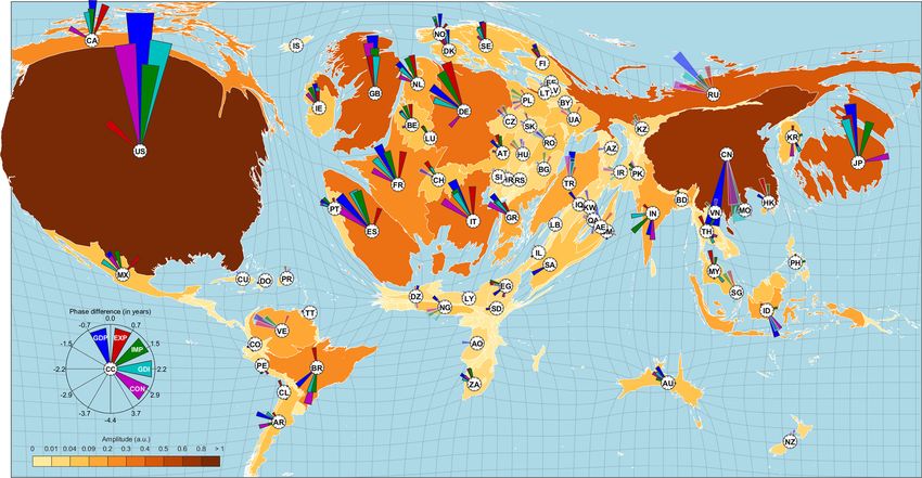
430                                                                                M. Ghil: Hilbert problems – 20 years later

of Ghil (2001) during the past 2 decades, from deterministi-      problems, whose number was increased to 23 in a sub-
cally autonomous to nonautononomous and random dynami-            sequent publication (Hilbert, 1900). In fact, of the prop-
cal systems (NDS and RDS; e.g., Ghil et al., 2008; Chekroun       erly formulated Hilbert problems, 10 problems, namely
et al., 2011; Bódai and Tél, 2012). This framework allows         {3, 7, 10, 11, 13, 14, 17, 19, 20, 21}, have a resolution that is
one to deal, in a self-consistent way, with the increasing role   accepted by a general consensus of the mathematical com-
of time-dependent forcing applied to the Earth system by hu-      munity. On the other hand, the solutions proposed for seven
manity and by natural processes, such as solar variability and    problems, namely {1, 2, 5, 9, 15, 18, 22}, are only partially
volcanic eruptions. Ghil (2019, Sect. 5.3) and Ghil and Lu-       accepted as resolving the corresponding problems.
carini (2019, Sect. IV.E) recently provided a fairly complete        That leaves problems 8 (the Riemann hypothesis), 12, and
review of these advances, and we shall thus mention them          16 unresolved, while 4 and 23 were too vaguely formulated
herein only in passing.                                           to ever be described as solved. Problem 6 is of particular in-
   The 10 problems proposed in Ghil (2001) to achieve this        terest to us here. Its overall heading (Hilbert, 1900) is the
goal were:                                                        “Mathematical treatment of the axioms of physics,” meaning
                                                                  that one should treat them in the same way as the “foun-
 1. What is the coarse-grained structure of low-frequency         dations of geometry”. This problem has been interpreted
    atmospheric variability, and what is the connection be-       as having the following two subproblems: (a) an axiomatic
    tween its episodic and oscillatory description?               treatment of probability that will yield limit theorems for the
                                                                  foundation of statistical physics, and (b) a rigorous theory
 2. What can we predict beyond 1 week, for how long, and          of limiting processes “which lead from the atomistic view
    by what methods?                                              to the laws of motion of continua,” e.g., from Boltzmann’s
 3. What are the respective roles of intrinsic ocean variabil-    equations of statistical mechanics to the partial differential
    ity, coupled ocean–atmosphere modes, and atmospheric          equations of continuous media. The mathematical commu-
    forcing in seasonal to interannual variability?               nity considers that the axiomatic formulation of the proba-
                                                                  bility theory by Kolmogoroff (2019) is an entirely satisfac-
 4. What are the implications of the answer to the previous       tory solution to part (a), although alternative formulations do
    problem for climate prediction on this timescale?             exist; part (b) is work in progress.
                                                                     On the contrary, problems in the physical sciences – let
 5. How does the oceans’ thermohaline circulation change          alone in the life sciences or socioeconomic sciences – cannot
    on interdecadal and longer timescales, and what is the        be “solved”, in general, to everybody’s satisfaction in finite
    role of the atmosphere and sea ice in such changes?           time. Apparently, though, social media do entertain the no-
                                                                  tion of “Hilbert problems for social justice warriors,” what-
 6. What is the role of chemical cycles and biological
                                                                  ever that may mean.
    changes in affecting climate on slow timescales, and
                                                                     The 10 original problems of Ghil (2001) could easily be
    how are they affected, in turn, by climate variations?
                                                                  complemented with 13 more, and the unanswered problems
 7. Does the answer to the question above give us some trig-      of the climate sciences would still be far from exhausted. We
    ger points for climate control?                               illustrate, instead, in the rest of this paper how attempts to
                                                                  solve four of the 10 problems above – namely problems 1,
 8. What can we learn about these problems from the atmo-         2, 3, and 10 – have fared over the intervening 2 decades and
    spheres and oceans of other planets and their satellites?     do so quite succinctly. Sections 2 and 3 deal with problems 1
                                                                  and 2 and with problem 3, respectively. Sections 4 and 5,
 9. Given the answers to the questions so far, what is the        in turn, address two complementary aspects of problem 10,
    role of humans in modifying the climate?                      namely the climate and coupling part versus the economic
                                                                  part. Concluding remarks follow in Sect. 6, and Appendix
10. Can we achieve enlightened climate control of our
                                                                  A provides some technical details on the results concerning
    planet by the end of the century?
                                                                  fluctuation–dissipation in macroeconomics.
   These problems were listed in increasing order of
timescale, from the shortest to the longest one, i.e., from
weeks to centuries and millennia. Ghil (2001) emphasized
the fact that, in mathematics, clearly formulated problems
can be given fully satisfactory solutions. Thus, in his “Lec-
ture delivered before the International Congress of Math-
ematicians at Paris in 1900,” David Hilbert2 proposed 10          Kurt-Otto Friedrichs–Richard Courant–David Hilbert, see https:
                                                                  //www.genealogy.math.ndsu.nodak.edu/id.php?id=33687 (last ac-
  2 The author of this paper is a great-great-grandson of         cess: 10 September 2020), but that is where any similarity or prox-
David Hilbert, through the sequence Michael Ghil–Peter D. Lax–    imity ends.

Nonlin. Processes Geophys., 27, 429–451, 2020                                        https://doi.org/10.5194/npg-27-429-2020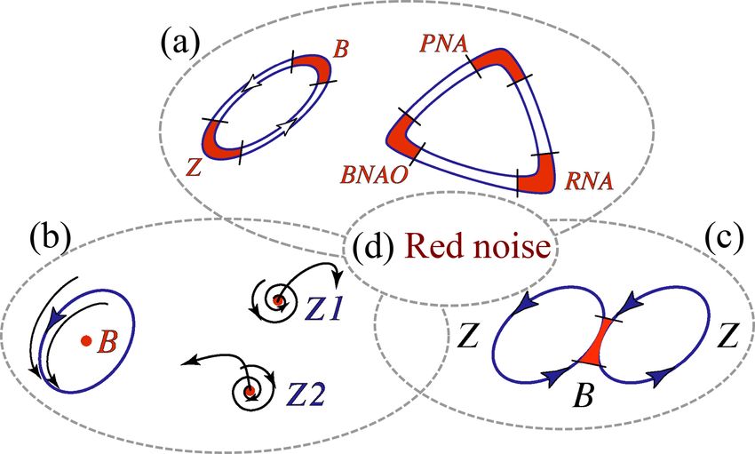
M. Ghil: Hilbert problems – 20 years later                                                                                    431

2   Problems 1 and 2: low-frequency atmospheric
    variability and medium-range forecasting

In the climate sciences, like in all the sciences, terms like
“low frequency” and “long term” have to be defined quanti-
tatively. The dominant frequency band in midlatitude day-to-
day weather is the so-called synoptic frequency of the evo-
lution of extratropical weather systems, which corresponds
to periodicities of 5–10 d. Thus, for the atmosphere, low-
frequency variability (LFV) and medium-range forecasting
refer to time intervals longer than 10 d.                         Figure 1. Schematic overview of atmospheric low-frequency vari-
   As recently mentioned in Ghil et al. (2018) and Ghil and       ability (LFV) mechanisms. Reprinted from Ghil et al. (2018), with
Lucarini (2019), it was John von Neumann (1903–1957), at          permission from Elsevier.
the very beginnings of climate dynamics, who made an im-
portant distinction (Von Neumann, 1960) between weather
and climate prediction. To wit, short-term numerical weather      (RNA), and the blocked phase of the North Atlantic Oscil-
prediction (NWP) is the easiest form of prediction, i.e., it is   lation (BNAO; Kimoto and Ghil, 1993a; Smyth et al., 1999).
a pure initial-value problem; long-term climate prediction is        Diagram (b) in Fig. 1 is associated with the idea of oscil-
the next easiest as it corresponds to studying the system’s       latory instabilities of one or more of the multiple fixed points
asymptotic behavior; intermediate-term prediction is hardest      that can play the role of regime centroids. Thus, Legras and
– both initial and boundary values are important. In this case,   Ghil (1985) found a 40 d oscillation due to a Hopf bifurcation
the boundary values refer mainly to the boundary conditions       off their blocked regime, B, while Z1 and Z2 in their model
at the air–sea and air–land interfaces.                           were generalized saddles that both had zonal flow patterns.
   Essentially, the first of the three problems above corre-      An ambiguity arises, though, between this point of view and
sponds to Lorenz’s predictability of the first kind, while        a complementary possibility, namely that the regimes are just
the second one corresponds to his predictability of the sec-      slow phases of such an oscillation, caused itself by the inter-
ond kind (Lorenz, 1967; Peixoto and Oort, 1992). It is the        action of the midlatitude jet with topography. Thus, Kimoto
intermediate-term prediction that requires going beyond the       and Ghil (1993b) found, in their observational data, closed
initial-value problem but without reaching all the way to a       paths within a Markov chain in which the states resemble
statistical equilibrium for very long times. It is this problem   well-known phases of an intraseasonal oscillation. Further-
that requires a unified treatment of slower climate change in     more, multiple regimes and intraseasonal oscillations can co-
the presence of faster climate variability, and we return to it   exist in a two-layer model on the sphere within the scenario
in Sects. 3 and 4.                                                of “chaotic itinerancy” (Itoh and Kimoto, 1997).
   Concerning the study of atmospheric LFV and medium-               Diagram (c) in Fig. 1 is a sketch of the linear point of view
range forecasting, Ghil (2001) had little to say about them       that persistent anomalies in midlatitude atmospheric flows
at the time. Both areas of inquiry, though, have taken huge       on 10–100 d timescales are just due to the slowing down of
strides over the last 2 or 3 decades (e.g., Kalnay, 2003;         Rossby waves or to their linear interference (Lindzen, 1986).
Palmer, 2017); the weather forecast for planning one’s holi-      An interesting extension of this approach into the nonlin-
day at the beach or in the mountains next week has become         ear realm is due to Nakamura and associates (Nakamura and
considerably more reliable. Still, a key issue associated with    Huang, 2018; Paradise et al., 2019). The traffic jam analogy
problem 1 was formulated by Ghil and Robertson (2002),            for blocking in this work is somewhat similar to the hydraulic
namely whether it is the “wave” point of view or the “par-        jump analogy of Rossby and collaborators (1939); see also
ticle” one that is more helpful in observing, describing, and     Malone et al. (1951/1955/2016, p. 432).
predicting LFV. To wit, is it (i) oscillatory modes with peri-       Finally, diagram (d) of Fig. 1 corresponds to the effects
ods of 30 d and longer, namely the waves, or (ii) persistent      of stochastic perturbations on any of the (a)–(c) scenarios
anomalies with durations of 10 d or longer and the Markov         (Hasselmann, 1976; Kondrashov et al., 2006; Palmer and
chains of transitions between more or less persistent regimes,    Williams, 2009).
namely the particles, that are more interesting and useful in        Recently, Lucarini and Gritsun (2020) made an interest-
coming to grips with medium-range forecasting?                    ing step in reconciling scenarios (a) and (b) in the fig-
   Ghil et al. (2018) have reformulated this problem more         ure. These authors used a fairly realistic, three-level quasi-
completely in Fig. 1. Here, diagram (a) represents Markov         geostrophic (QG3) model (Marshall and Molteni, 1993; Kon-
chains between two or more flow regimes with distinct spa-        drashov et al., 2006) to study blocking events through the
tial patterns and stability properties, such as blocked (B)       lens of unstable periodic orbits (UPOs; Cvitanović and Eck-
and zonal (Z; Charney and DeVore, 1979, and references            hardt, 1989; Gilmore, 1998). UPOs are natural modes of vari-
therein) or Pacific–North-American (PNA), Reverse PNA             ability that densely populate a chaotic system’s attractor. Lu-

https://doi.org/10.5194/npg-27-429-2020                                       Nonlin. Processes Geophys., 27, 429–451, 2020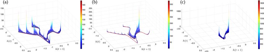
432                                                                               M. Ghil: Hilbert problems – 20 years later

carini and Gritsun (2020) found that blockings occur when         evolution of the latter point of view in the study of oceanic
the system’s trajectory is in the neighborhood of a specific      interannual variability here.
class of UPOs.                                                       A paradigmatic example of how complex intrinsic LFV
   The UPOs that correspond to blockings in the QG3 model         can arise in the ocean circulation is the so-called double-
are more unstable than the UPOs associated with zonal flow;       gyre problem (e.g., Ghil et al., 2008; Ghil, 2017). Note that
thus, blockings are associated with anomalously unstable at-      the synoptic timescale in the oceans is associated with the
mospheric states, as suggested theoretically by Legras and        oceanic counterpart of “weather” – i.e., with the lifetime of
Ghil (1985) and confirmed experimentally in a rotating annu-      so-called mesoscale eddies – and it is of months rather than a
lus with bottom topography by Weeks et al. (1997); see also       week or two (Gill, 1982; Pedlosky, 1996). Hence, LFV in the
Ghil and Childress (1987/2012, chap. 6). Different regimes        ocean corresponds to several years rather than to 1–3 months.
(particles) may be associated with different bundles of UPOs         Veronis (1963) already obtained the bistability of steady
(waves).                                                          solutions in a single-gyre configuration and a stable limit cy-
   Given this perspective on atmospheric LFV, what can be         cle for time-independent wind stress. Jiang et al. (1995) stud-
said about the predictability of flow features in the 10–100 d    ied the successive bifurcation tree all the way to chaotic so-
window between the limit of detailed, deterministic pre-          lutions in a double-gyre model with steady time-independent
dictability, on the one hand (e.g., Lorenz, 1969), and the        forcing. The periodic solutions they obtained were plurian-
large changes induced in the atmospheric circulation by the       nual, had the characteristics of relaxation oscillations, and
march of seasons, on the other? Clearly, the occurrence of        were termed gyre modes because of the strong vortices they
certain flow patterns that are more frequently observed, and      exhibited on either side of the separation of the model’s
thus associated with clusters or regimes, should be more pre-     eastward jet from the western boundary (Dijkstra and Ghil,
dictable. The relative success of Markov chains in describing     2005).
the transitions between qualitatively different regimes is con-      Pierini et al. (2016, 2018) applied, to simplified double-
sistent with the results of Lucarini and Gritsun (2020).          gyre models, the previously mentioned NDS theory. These
   Ghil et al. (2018) have carried out a detailed review of       authors found that, even in the presence of time-dependent
many studies on what used to be called intraseasonal atmo-        forcing and of a unique global pullback attractor (PBA), two
spheric variability and is more recently being called subsea-     local PBAs with very different stability properties can co-
sonal to seasonal (S2S) variability. They concluded that the      exist, and their mutual boundary appears to be fractal; see
number and variety of methods that have been used to iden-        Fig. 2 here and the more detailed explanations in Ghil (2019,
tify and describe LFV regimes are leading up to a tentative       Fig. 12). Ghil (2017) and Ghil and Lucarini (2019) reviewed
consensus on their existence, robustness, and characteristics.    both the fundamental ideas of NDS and RDS theory and their
S2S forecasting has become operationally viable and is un-        applications to climate problems; hence, little more will be
der intensive investigation (e.g., Robertson and Vitart, 2018,    said herein on these topics.
and references therein).                                             Feliks et al. (2004, 2007) showed that a narrow and suf-
                                                                  ficiently strong SST front with the 7 year periodicity of the
                                                                  oceanic gyre modes could give rise to a similar near period-
3   Problem 3: oceanic interannual variability                    icity in the atmospheric jet stream above the oceanic east-
                                                                  ward jet, provided the resolution of the atmospheric model
A remarkable feature of human nature is the tendency to al-       was sufficiently high; see also Minobe et al. (2008). Groth
ways put the blame elsewhere – rather than at one’s own           et al. (2017) studied reanalysis fields for both ocean and at-
doorstep. Thus, meteorologists tended to blame sea surface        mosphere over the North Atlantic basin and adjacent land
temperatures (SSTs) for changes in atmospheric circulation        areas (25–65◦ N, 80–0◦ W); they found their results to be in
on S2S timescales and longer, while oceanographers blamed         good agreement with the dominant 7–8 year periodicity of
changes in the wind stress for such changes in the upper          the North Atlantic Oscillation (NAO) being due to the intrin-
ocean. It is more judicious, though, to ask “What are the re-     sic periodicity of barotropic gyre modes. The agreement with
spective roles of intrinsic ocean variability, coupled ocean–     the alternative theory of a turbulent oscillator (Berloff et al.,
atmosphere modes, and atmospheric forcing in seasonal to          2007) playing a key role in the NAO was less evident since
interannual variability?” as done in problem 3 of Ghil (2001).    the latter depends, in an essential way, on strong baroclinic
   The difference between the two approaches is largely one       activity and has a much broader spectral peak that does not
between linear thinking, in which changes in a system at          emphasize the NAO’s 7–8 year peak.
frequencies not present in its free modes have to be due to          On the other hand, Vannitsem et al. (2015) investigated
external agencies, and nonlinear thinking, in which combi-        oceanic LFV in a coupled ocean–atmosphere model with
nation tones and other more complex spectral features may         a total of 36 Fourier modes. Their results included stable
be present. Moreover, interactions between subsystems and         decadal-scale periodic orbits with a strong atmospheric com-
between any subsystem and time-dependent forcing can be           ponent, and chaotic solutions that were still dominated by
much richer in a nonlinear world. We will briefly sketch the      the decadal behavior. Projecting atmospheric and oceanic re-

Nonlin. Processes Geophys., 27, 429–451, 2020                                        https://doi.org/10.5194/npg-27-429-2020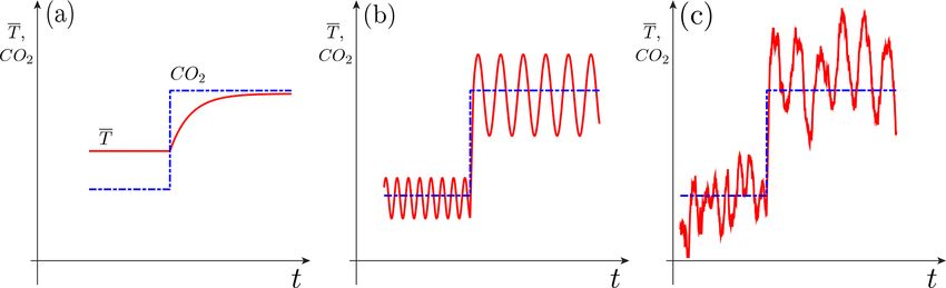
M. Ghil: Hilbert problems – 20 years later                                                                                                433

Figure 2. Numerical evidence for the existence of two local pullback attractors (PBAs) in the wind-driven midlatitude ocean circulation.
Plotted is a mean normalized distance, 1, for 15 000 trajectories of the double-gyre ocean model of Pierini et al. (2016, 2018); the cold
colors correspond to very quiescent behavior, while the warm colors are associated with unstable, chaotic motion on the PBA. The parameter
values in the two panels are, respectively, subcritical and supercritical in the autonomous version of the model with respect to the homoclinic
bifurcation that gives rise to relaxation oscillations in the latter – (a) γ = 0.96 and (b) γ = 1.1. Reproduced from Pierini et al. (2016). ©
American Meteorological Society; used with permission.

analysis data sets onto the leading modes of the Vannitsem                dictability, rather than merely pushing it to higher and higher
et al. (2015) model, Vannitsem and Ghil (2017) confirmed                  resolutions in order to achieve ever more detailed simulations
that a dominant LFV signal with a 25–30 year period (Tim-                 of the system’s behavior for a limited set of semiempirical
mermann et al., 1998; Frankcombe and Dijkstra, 2011) is a                 parameter values.
common mode of variability of the atmosphere and oceans.
   Clearly, the separation between the wind-driven circula-
tion addressed by problem 3 and the buoyancy-driven circu-                4     Problem 10A: climate change and its control – a path
lation addressed by problem 5 is rather a matter of conve-                      to integrated thinking
nience as a water particle in the ocean is affected by both
types of forces. Moreover, recently, Cessi (2019, and refer-              4.1    Background
ences therein) have argued that the meridional overturning
is actually powered by momentum fluxes and not by buoy-                   Much more has been done about this ultimate problem over
ancy fluxes. This argument is not quite generally accepted;               the last 2 decades than over the two previous ones. First of
see, for instance, Tailleux (2010). Given the lack of consen-             all, it has become obvious that we cannot wait until the end
sus about the matter, the thermohaline circulation of problem             of the century to achieve enlightened control over the cli-
5 is increasingly termed the oceans’ meridional overturning               mate. The attribute “enlightened” plays a crucial role here; it
circulation, thus avoiding a definite attribution of its physical         clearly does not include rather crude geoengineering propos-
causes.                                                                   als that risk doing as much harm as, or more harm than, good.
   In the studies of atmospheric, oceanic, and coupled vari-              The field of geoengineering has blossomed, though, and we
ability of the climate system, considerable progress has been             merely refer here to a recent critique of some of the more
made in applying dynamical systems theory and, in partic-                 misguided proposals (Bódai et al., 2020); see also Ghil and
ular, bifurcation theory to models subject to time-dependent              Lucarini (2019, Sect. IV.E.4).
forcing (Alkhayuon et al., 2019) or to models that lie fur-                  Some combination of a reduction in greenhouse gas emis-
ther towards the high end (Rahmstorf et al., 2005; Hawkins                sions, an increase in capture and sequestration, and a variety
et al., 2011) of the model hierarchy originally proposed by               of adaptation and mitigation strategies has to be implemented
Schneider and Dickinson (1974). More recently, Ghil (2001)                to avoid the most dire consequences of anthropogenic cli-
and Held (2005), among others, have emphasized the need                   mate change (Stern, 2007; Nordhaus, 2013; IPCC, 2014b).
to pursue such a hierarchy systematically in order to further             Large uncertainties, however, remain and have to be taken
increase understanding of the climate system and of its pre-              into account both in the decision-making processes leading

https://doi.org/10.5194/npg-27-429-2020                                                Nonlin. Processes Geophys., 27, 429–451, 2020
434                                                                                    M. Ghil: Hilbert problems – 20 years later

to near-optimal and affordable strategies and in the imple-          risk FAR as follows:
mentation thereof.
                                                                     FAR = 1 − p0 /p1 .                                          (1)

4.1.1   Detection and attribution (D&A) studies                      We skip here several important steps in causality theory that
                                                                     involve comparing directed dependency graphs when one is
                                                                     interested in more than one possible effect – e.g., a dust
Before addressing these issues, it is worth mentioning that          devil and a hailstorm – and more than one cause may be at
important strides have been taken in the field of detection          play, such as the values of the temperature field and those of
and attribution (D&A) of individual events to climate change         the wind field in some neighborhood of the observed event.
(Stone and Allen, 2005; Hannart et al., 2016b). To start,            Please see Hannart et al. (2016b, Fig. 1), and the discussion
changes in global quantities that involve averaging over large       thereof, and Pearl (2009b, Sect. 2).
spans of time and large areas of the globe have been both               The key mathematical novelty in Pearl’s counterfactual
detected in and attributed to, with considerable confidence,         theory of causation is the realization that, following Hume,
anthropogenic changes in the atmospheric concentration of            a cause should be both necessary and sufficient in order to
aerosols and greenhouse gases (IPCC, 2014a, b). The D&A              unambiguously attribute an observed event to it. Instead of
of regional changes (e.g., Stott et al., 2010) and, a fortiori, of   merely computing the fraction of attributable risk, FAR , as
individual events (e.g., Hannart et al., 2016a) is considerably      in Eq. (1), one needs to define and compute the probabilities
more difficult and much less incontrovertible.                       PN , PS , and PNS of necessary, sufficient, and necessary and
   Given the substantial impact of extreme events on human           sufficient causation.
life and socioeconomic well-being (e.g., Ghil et al., 2011;             Thus, the probability, PN , of necessary causation is defined
Chavez et al., 2015; Lucarini et al., 2016), an important step       as the probability that the event, Y , would not have occurred
in achieving greater rigor in this field is a greater reliance       in the absence of the event, X, given that both events, Y and
on the counterfactual theory of necessary and sufficient cau-        X, did in fact occur. Sufficient causation, on the other hand,
sation, formulated by Judea Pearl (Pearl, 2009a, b), in the          means that X always triggers Y but that Y may also occur for
attribution of such events.                                          other reasons without requiring X. Finally, PNS is the prob-
   The counterfactual definition of causality goes back to the       ability that a cause is both necessary and sufficient. These
Scottish Enlightenment philosopher, historian, economist,            three definitions are formally expressed as follows:
and essayist David Hume (1711–1776), widely remembered
for his empiricism and skepticism. It can be stated simply as        PN ≡ P (Y0 = 0|Y = 1, X = 1),                              (2a)
follows: Y is caused by X if, and only if, Y would not have          PS ≡ P (Y1 = 1|Y = 0, X = 0),                              (2b)
occurred were it not for X.                                          PNS ≡ P (Y0 = 0, Y1 = 1).                                  (2c)
   The usual identification of Pearl’s causal theory as “coun-
terfactual” appears to be, at first glance, rather counterintu-      Recall that the subscript 1 refers to the factual world, while
itive. We take, therefore, a little detour here to explain briefly   the subscript 0 refers to the counterfactual one; see Eq. (1).
the theory and outline how it differs from the usual approach           The definitions in Eq. (2) are precise and unambiguously
taken so far in D&A studies (Allen, 2003; Stone and Allen,           implementable, as long as a fully specified probabilistic
2005). In doing so, we follow Hannart et al. (2016b).                model of the world is formulated. Under certain assumptions,
   An individual event is characterized by a binary variable,        spelled out by Hannart et al. (2016b), the probabilities PN ,
Y ∈ {0, 1}, and, say, the threshold exceedance of surface air        PS , and PNS can be calculated as follows:
temperatures for a time interval, τ , and over an area, A. For                  p0                 1 − p1
brevity, we will use the “event Y ” as a stand-in for the event      PN = 1 −      ,    PN = 1 −          ,   PNS = p1 − p0 .    (3)
                                                                                p1                 1 − p0
defined by {Y = 1}. The idea of causation of Y by a differ-
ence f ∈ F in the forcing – with F representing a set of val-        One can easily see that PN is more sensitive to p0 than to p1 ,
ues of insolation, atmospheric composition, etc. – is to distin-     and, conversely, that PS is more sensitive to p1 than to p0 ;
guish between a situation in which f has the value measured          necessary causation is enhanced further by an event being
during Y in the real, or factual, world, and the value f = 0         rare in the counterfactual world, whereas sufficient causation
that it would have had in an alternative, or counterfactual,         is enhanced further by it being frequent in the factual one;
world. The presence or absence of the extra forcing, f , is          see, for instance, Hannart et al. (2016b, Fig. 2).
captured by another binary variable, Xf .                               An interesting idea – first articulated by Hannart et al.
   Obviously, the distinction between the two situations re-         (2016b) and further implemented by Carrassi et al. (2017)
quires one to estimate the probability, p1 = P (Y = 1|Xf =           – is to apply data assimilation methodology (e.g., Bengts-
1), of the event occurring in the factual world and the proba-       son et al., 1981; Ghil and Malanotte-Rizzoli, 1991; Kalnay,
bility, p0 = P (Y = 1|Xf = 0), of it occurring in the counter-       2003) for the computation of these three probabilities, using
factual world. The prevailing approach is to, given estimates        observations from the factual world and a model that encap-
p1 and p0 , t compute the so-called fraction of attributable         sulates the knowledge of the system’s evolution. One uses

Nonlin. Processes Geophys., 27, 429–451, 2020                                            https://doi.org/10.5194/npg-27-429-2020
M. Ghil: Hilbert problems – 20 years later 435
two versions of the latter model, namely the factual one with use models with this marked deficiency to predict future cli-
Xf = 1 and the other one with Xf = 0, and the data are sup- mates on multidecadal timescales.
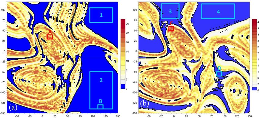
posed to tell one whether PNS is sufficiently close to unity or Concerning the ENSO’s distribution of extreme events,
not. Ghil and Zaliapin (2015) investigated its dependence, in an
idealized delay differential equation (DDE) model, on sev-
4.1.2 Beyond equilibrium climate sensitivity eral model parameters. They also found that plotting the
model’s PBA, with respect to the seasonally periodic forc-
Returning now to the issues of near-optimal control of cli- ing, provided a much better understanding of the role of the
mate change, it is important to realize that what needs to be seasonal cycle in the model.
controlled is not just the global and annual mean surface air Chekroun et al. (2018) found that parameter dependence in
temperature, T , as originally studied in the Charney et al. such a DDE model can lead to a critical transition between
(1979) report. To outline the progress made in the 4 decades two types of chaotic behavior which differ substantially in
since the Charney report in thinking about anthropogenic ef- their distribution of extreme events. This contrast is clearly
fects on climate, please consider Fig. 3 herein. apparent in Fig. 4, and it illustrates the types of nonequilib-
The figure is a highly simplified conceptual diagram of rium climate changes suggested by Fig. 3c.
the way that anthropogenic changes in radiative forcing The changes in the invariant, time-dependent measure, µt ,
would change the behavior of a climate system with increas- supported on this ENSO model’s PBA are plotted in Fig. 4a–
ingly complex characteristics, as one proceeds from Fig. 3a c as a function of the control parameter a. The change in the
through Fig. 3b and on to Fig. 3c. Therefore, neither the time, PBA is clearly associated with the population lying towards
t, on the abscissa nor the CO2 concentration and temperature, the ends of the elongated filaments apparent in the figure.
T , on the ordinate are labeled quantitatively in the three pan- This population represents strong, warm El Niño and cold
els. The time we think of is years to decades, and the ranges La Niña events.
of the CO2 concentration and T correspond roughly to those The PBA experiences a critical transition at a value, a∗ ;
expected for the difference in values between the end of the here, h(t) is the thermocline depth anomaly from seasonal
21st century and the beginning of the 19th century. To keep depth values at the domain’s eastern boundary, with t in
things as simple as possible – but definitely not any simpler years; a = (1.12 + δ))/180 and 0.015700 < δ∗ < 0.015707.
– anthropogenic changes in radiative forcing have been rep- Thus, µt (a) faithfully encrypts the disappearance of such ex-
resented by a sudden jump in CO2 concentration, as in the treme events as a % a∗ . Adding stochastic perturbations to
Charney report. the model can smooth out the transition, which might make
The climate model represented in the Fig. 3a can be as it less drastic in high-end models and in observations. Again,
simple as a forced linear, scalar, ordinary differential equa- the study of the model’s PBA greatly facilitates the under-
tion representing an energy balance model, as follows: standing of the processes involved.
ẋ = −λx + H (t)(x − x1 ), x(t) ≡ T (t) − T 0 , (4) 4.2 Integrated assessment models (IAMs)
with λ > 0, and H (t) a Heaviside function that jumps from So-called integrated assessment models (IAMs) have been,
H = 0, for t ≤ 0, to H = 1, for t > 0. Here T 0 and T 1 are so far, the main tool for assessing the future impact of climate
the model’s equilibrium climates for the radiative forcings change on the global economy and, even more ambitiously,
before and after the jump, respectively, while λ gives the rate on one or more regional ones (e.g., Stern, 2007; Nordhaus,
of exponentially approaching the new equilibrium T 1 . 2014; Clarke et al., 2014; IPCC, 2014b; Hughes, 2019). The
The case of Fig. 3b can be seen as an idealized climate main purpose of IAMs is to provide reasoned scientific input
system in which the El Niño–Southern Oscillation (ENSO) into major socioeconomic and political decisions that will af-
would be perfectly periodic, rather than having an irregu- fect both the present and future generations of humanity, as
lar, 2–7 year periodicity with additional periodicities and well as planet Earth as a whole. In doing so, IAMs attempt
chaotic components present, as in Fig. 3c. There are no se- to weigh the cost and effectiveness of competing or com-
rious doubts as to the long-term mean, T 1 , after the jump plementary adaptation and mitigation measures by applying
being larger than the preindustrial or current mean, T 0 . But, various methods of cost–benefit analysis (Clarke et al., 2014;
figuring out the higher moments of the long-term probability IPCC, 2014b; Hughes, 2019) and decision theory (e.g., Bar-
density function (pdf) after the jump is another matter en- nett et al., 2020, and references therein).
tirely. IAMs attempt to link major features of economy and so-
Recently, increasing attention has been paid by high-end ciety with the climate system and biosphere into one mod-
modelers to the difficulties posed by the presence of internal eling framework, a lofty purpose that clearly has to over-
variability in the climate system. For instance, Deser et al. come major obstacles. Some of the obstacles have to do with
(2020, and references therein) point to this variability’s im- the complexity of the coupled system’s distinct components,
perfect simulation and to the consequences of attempting to others with the different cultures and research styles of the
https://doi.org/10.5194/npg-27-429-2020 Nonlin. Processes Geophys., 27, 429–451, 2020436 M. Ghil: Hilbert problems – 20 years later Figure 3. Schematic diagram of the effects of a sudden change in atmospheric carbon dioxide (CO2 ) concentration (blue dashed and dotted line) on seasonally and globally averaged surface air temperature T (red solid line). Climate sensitivity is shown (a) for an equilibrium model, (b) for a nonequilibrium oscillatory model, and (c) for a nonequilibrium chaotic model, possibly including random perturbations. As radiative forcing (atmospheric CO2 concentration, say) changes suddenly, global temperature (T ) undergoes a transition. In panel (a) only the mean temperature changes, in panel (b) the mean adjusts, as it does in panel (a), but the period, amplitude, and phase of the oscillation can also decrease, increase, or stay the same, while in panel (c) the entire intrinsic variability changes as well, including the distribution of extreme events. From Ghil (2017); used with permission from the American Institute of Mathematical Sciences, under the Creative Commons Attribution license. Figure 4. Critical transition in extreme event distribution in an idealized El Niño–Southern Oscillation (ENSO) model. The invariant, time- dependent measure, µt , supported on the PBA of the ENSO delay differential equation (DDE) model of Tziperman et al. (1994), is plotted here via its embedding into the (h(t), h(t +1)) plane for a = (1.12+δ))/180 and t ' 147.64 yr and, respectively, (a) δ = 0.0, (b) δ = 0.01500, and (c) δ = 0.015707. The red curves in the three panels represent the singular support of the measure. Reprinted with permission from Chekroun et al. (2018). scientific communities involved. Finally, the data sets neces- General equilibrium theory is a cornerstone of today’s sary for estimating model parameters are short, incomplete, mainstream economics, often referred to as neoclassical eco- and often rather inaccurate. The United Nation’s Intergovern- nomics (Aspromourgos, 1986). This theory relies heavily on mental Panel on Climate Change (IPCC) has dedicated sub- equilibrium in both the labor and product markets; prices of stantial efforts over the last 3 decades to overcoming these goods and wages of labor are assumed to be flexible and to various obstacles (IPCC, 1990, 2001, 2007, 2014a, b). adjust so as to achieve equilibrium in the product and labor Mostly, IAMs have used both climate and economic mod- markets at all times. As a result, it is possible to maximize ules that were conceived in the spirit of Fig. 3a, i.e., (i) of an intergenerational utility functional, following the planning so-called equilibrium climate sensitivity (ECS), as studied by approach of Ramsey (1928). Moreover, the mean growth of Charney et al. (1979) 4 decades ago, for the climate module the economy (Solow, 1956) is only perturbed by exogenous and (ii) of general equilibrium theory (Walras, 1874/1954; shocks that lead to random fluctuations reverting to a stable Pareto, 1919; Arrow and Debreu, 1954), going back to the equilibrium, which can be modeled by auto-regressive pro- late 19th century, for the economic module. We have consid- cesses of order 1, called AR(1) processes. ered, in Sects. 2 and 3 above, how to formulate a more active The economic modules of most IAMs used so far in the climate module that might behave more like Fig. 3b, or even IPCC process (e.g., IPCC, 2014b, and references therein) like Fig. 3c, given changes in radiative forcing induced by rely on general equilibrium theory and its consequences. anthropogenic emissions of greenhouse gases and aerosols. These IAMs differ largely by the values they prescribe for For illustrative purposes, we will merely sketch a highly ide- various parameters; among the latter, the most important one alized counterpart of such behavior for the economic module is the discount factor, which essentially gives the future value of an IAM. of a currency unit versus its value today. Large differences Nonlin. Processes Geophys., 27, 429–451, 2020 https://doi.org/10.5194/npg-27-429-2020
M. Ghil: Hilbert problems – 20 years later                                                                                     437

among the value of this factor, assumed in the work of Stern        5     Problem 10B: nonequilibrium economics,
(2007) versus that of Nordhaus (2014), for instance, have                 fluctuation–dissipation, and synchronization
lead to very different conclusions about the mitigation poli-
cies recommended by these two authors.                              5.1    Nonequilibrium economic models and a
    More generally, Wagner and Weitzman (2015, among oth-                  vulnerability paradox
ers) have emphasized how uncertainty in the climate sys-
tem’s dynamics could create fat-tailed distributions of poten-      There is no denying that, superimposed on overall global
tial damages, while Pindyck (2013) and Morgan et al. (2017)         growth in economic activity, ups and downs are as well
find existing IAMs to be of little value in providing scien-        known as recessions and upswings. These short-term varia-
tific guidance for the formulation of prudent adaptation and        tions may appear only as small wiggles on a long-term expo-
mitigation policy. More radically, Davidson (1991) already          nential tendency of economic indicators, like gross domestic
questioned the extent to which certain types of economic un-        product (GDP), but they are quite severe in the individual ex-
certainties could be represented judiciously by probabilistic       perience of households, firms, countries, and even the world
approaches, as has been done routinely in the IAMs’ estima-         as a whole. There are two rather distinct approaches to mod-
tion of utility functionals associated with the system’s future     eling these so-called business cycles, namely the “real” busi-
trajectories. Farmer et al. (2015) have also emphasized the         ness cycle (RBC) theory and the endogenous business cycle
need for better uncertainty estimates and better accounting         (EnBC) theory. The “real” in RBC theory refers to the fact
for technological change and for heterogeneities in the cou-        that the theory explains macroeconomic fluctuations as the
pled system as well as for more realistic damage functions.         result of real productivity shocks and does not emphasize the
    More specifically, Barnett et al. (2020) have recently em-      monetary or financial aspects of the economy. A good start-
phasized that the uncertainties associated with assessing the       ing point for this literature is Brock and Mirman (1972).
future impact of climate change, and, hence, with devising             RBC theory is closely tied to the mainstream economics
adaptation and mitigation policies, go well beyond the well-        approach (Kydland and Prescott, 1982) in which the expec-
known uncertainties in the discount factor and in other pa-         tations of households and firms are rational, supply equals
rameters of either the climate or the economic module of cou-       demand, and there is no involuntary unemployment. In RBC
pled models. They suggest the following three much broader          models, the fluctuations are entirely due to external, exoge-
types of uncertainties:                                             nous shocks, and the models’ response to such shocks is
                                                                    purely via AR(1) processes. This theory is adopted by a very
  i. Risk – uncertainty within a model, which involves un-          large fraction of practicing economists, and many modifica-
     certain outcomes with known probabilities                      tions to it have tried to bring it in closer agreement with the
 ii. Ambiguity – uncertainty across models, which arises            observed behavior of real economies (e.g., Hoover, 1992).
     from unknown weights for alternative possible models           One way this approach has been criticized is that it describes
                                                                    the world as it ought to be, rather than how it is, and consid-
 iii. Misspecification – uncertainty about models, which in-        erable controversy still exists as to its explanation of major
      volves unknown flaws of approximating models.                 aspects of observed macroeconomic fluctuations (e.g., Sum-
                                                                    mers, 1997; Romer, 2011).
It is worth considering, in this context, the uncertainties as-        In contradistinction, EnBC theory relies on a number
sociated with the economic counterpart of natural or intrin-        of heterodox – i.e., nonconformist – economic ideas, most
sic variability in the climate system; such variability is called   importantly on post-Keynesian economics (Kalecki, 1935;
endogenous in the economic literature. Following a parallel         Keynes, 1936/2018; Malinvaud, 1977). EnBC theory ac-
line of reasoning, Hallegatte (2005) argued for closed-loop         knowledges at least some of the imperfections of real
climate–economy modeling, i.e., a two-way feedback inter-           economies up front; in this theory, economic fluctuations are
action that also accounts for multiple timescales in both mod-      due to intrinsic processes that endogenously destabilize the
ules. We turn, therewith, to the economic part of the model-        economic system (Kalecki, 1935; Samuelson, 1939; Flaschel
ing and data analysis, as it is highly pertinent to a truly in-     et al., 1997; Chiarella et al., 2005) and often involve delays
tegrated way of thinking about the Earth system, including          among economic processes. Even Hayek, a leading liberal,
the humans that affect it more and more – whatever the exact        anti-Keynesian economist, had interesting ideas on the de-
time at which the Anthropocene (Crutzen, 2006) might have           lays between decision and implementation time in invest-
started (Lewis and Maslin, 2015).                                   ments (Hayek, 1941/2007).
                                                                       At this point it might be worth noting that, in equilibrium
                                                                    macroeconomic models, output is supply driven, while in
                                                                    nonequilibrium models it is demand driven, a feature that is
                                                                    inherited from the corresponding models that attempt to as-
                                                                    sess climate damage. An interesting recent example of the
                                                                    latter is the post-Keynesian Dynamic Ecosystem-FINance-

https://doi.org/10.5194/npg-27-429-2020                                          Nonlin. Processes Geophys., 27, 429–451, 2020
438 M. Ghil: Hilbert problems – 20 years later
Economy (DEFINE) model, which explicitly includes banks
in addition to firms and households (Dafermos et al., 2018).
5.1.1 The nonequilibrium dynamic model of Hallegatte
et al. (2008)
We present here, concisely, one particular EnBC model, and
the role that active economic dynamics may have in modify-
ing the effect of natural hazards on such an economy (Halle-
gatte and Ghil, 2008). The nonequilibrium dynamical model
(NEDyM) of Hallegatte et al. (2008) is a neoclassical model
based on the Solow (1956) model, in which equilibrium con-
straints associated with the clearing of goods and labor mar-
kets are replaced by dynamic relationships that involve ad-
justment delays. The model has eight state variables – which
include production, capital, number of workers employed, Figure 5. Bifurcation diagram of a nonequilibrium dynamical
wages, and prices – and the evolution of these variables is model (NEDyM), showing its transitions from equilibrium to purely
modeled by a set of ordinary differential equations. For a periodic and on to chaotic behavior. The investment parameter αinv
brief summary of the model equations, please see Groth et al. is on the abscissa, and the investment ratio 0inv is on the ordinate.
(2015a, Appendix A); the parameters and their values are The model has a unique, stable equilibrium for low values of αinv ,
listed in Hallegatte et al. (2008, Table 3). with 0inv ' 0.3. A Hopf bifurcation occurs at αinv ' 1.39, leading
NEDyM’s main control parameter is the investment flex- to a limit cycle, followed by transition to chaos at αinv ' 3.8. The
ibility αinv , which measures the adjustment speed of invest- crosses indicate first the stable equilibrium and then the orbit’s min-
ima and maxima, while dots indicate the Poincaré intersections with
ments in response to profitability signals. This parameter de-
the hyperplane, H = 0, when the goods inventory, H , vanishes. Re-
scribes how rapidly investment can react to a profitability sig-
produced from Groth et al. (2015a), with permission from AGU
nal. If αinv is very large, investment soars when profits are Wiley.
high and collapses when profits are small, while a small αinv
entails a much slower adjustment of the investment to the
size of the profits. Introducing this parameter is equivalent
to allocating an investment adjustment cost, as proposed by
Kydland and Prescott (1982) and by Kimball (1995); these and recoveries of variable duration. In the present paper, we
authors found that introducing adjustment costs and delays concentrate, for the sake of simplicity, on model behavior in
helps to match the key features of macroeconomic models to the purely periodic regime, i.e., we have regular EnBCs but
the data. no chaos. Such periodic behavior is illustrated in Fig. 6.
In NEDyM, for small αinv , i.e., slow adjustment, the model The NEDyM business cycle is consistent with many styl-
has a stable equilibrium, which was calibrated to the eco- ized facts described in macroeconomic literature, such as the
nomic state of the European Union (EU-15) in 2001 (Eu- phasing of the distinct economic variables along the cycle,
rostat, 2002). As the adjustment flexibility increases, this with the distinct phrases being referred to in this literature
equilibrium loses its stability and undergoes a Hopf bifurca- as comovements. The model also reproduces the observed
tion, after which the model exhibits a stable periodic solution asymmetry of the cycle, with recessions that are much shorter
(Hallegatte et al., 2008). than expansions. This typical sawtooth shape of a business
Business cycles in NEDyM originate from the instability cycle is not well captured by RBC models, whose linear,
of the profit–investment feedback, which is quite similar to auto-regressive character gives intrinsically symmetric be-
the Keynesian accelerator–multiplier effect. Furthermore, the havior around the equilibrium. The amplitude of the price–
cycles are constrained and limited in amplitude by the in- wage oscillation, however, is too large in NEDyM, calling
terplay of the following three processes: (i) a reserve army for a better calibration of the parameters and further refine-
of labor effect, namely labor costs increasing when the em- ments of the model.
ployment rate is high, (ii) the inertia of production capacity, In the setting of the 2008 economic and financial crisis, the
and (iii) the consequent inflation in goods prices when de- banks’ and other financial institutions’ large losses clearly re-
mand increases too rapidly. The model’s bifurcation diagram duced access to credit; such a reduction very strongly affects
is shown in Fig. 5. investment flexibility. The EnBC model can thus help explain
For somewhat greater investment flexibility, the model ex- how changes in αinv can seriously perturb the behavior of
hibits chaotic behavior because a new constraint intervenes, the entire economic system, either by increasing or decreas-
namely limited investment capacity. In this chaotic regime, ing the variability in macroeconomic variables; see Fig. 5.
the cycles become quite irregular, with sharper recessions Moreover, these losses also lead to a reduction in aggregated
Nonlin. Processes Geophys., 27, 429–451, 2020 https://doi.org/10.5194/npg-27-429-2020M. Ghil: Hilbert problems – 20 years later 439
modest due to the fact that the country was experiencing a
strong recession of −7 % of the GDP in the year before the
disaster (World Bank, 2003).
To study how the state of the economy may influence the
consequences of natural disasters, Hallegatte and Ghil (2008)
introduced into NEDyM the disaster-modeling scheme of
Hallegatte et al. (2007), in which natural disasters destroy the
productive capital through a modified production function.
Furthermore, to account for market frictions and constraints
in the reconstruction process, the reconstruction expenditures
are limited.
These authors showed that the transition from an equilib-
rium regime to a nonequilibrium regime can radically change
the long-term response to exogenous shocks in an EnBC
model. Idealized as it may be, NEDyM shows that the long-
term effects of a sequence of extreme events depend upon the
economy’s behavior; an economy in stable equilibrium with
very little, or no, flexibility (αinv . 0.5, see Fig. 5) is more
vulnerable than a more flexible economy, albeit still at or near
equilibrium (e.g., αinv ' 1.0). Clearly, if investment flexibil-
ity is nil or very low, the economy is incapable of responding
to the natural disasters through investment increases aimed
at reconstruction; total production losses, therefore, are quite
large. Such an economy behaves according to a pure Solow
(1956) growth model, where the savings, and therefore the
investment, ratio is constant; see Hallegatte and Ghil (2008,
Table 1).
Figure 6. Endogenous limit cycle behavior of NEDyM for an in- When investment can respond to profitability signals with-
vestment flexibility of αinv = 2.5; for all other parameter values, out destabilizing the economy, i.e., when αinv is nonzero but
please see Hallegatte et al. (2008, Table 3). Reproduced from Groth still lower than the critical bifurcation value of αinv ' 1.39,
et al. (2015a), with permission from AGU Wiley.
the economy has greater freedom to improve its overall state
and, thus, respond to productive capital influx. Such an econ-
demand that, in turn, can lead to a reduction in economic omy is much more resilient to disasters because it can adjust
production and a full-scale recession. its level of investment in the disaster’s aftermath.
If investment flexibility, αinv , is larger than its Hopf bifur-
5.1.2 Regime-dependent effect of climate shocks cation value, the economy undergoes periodic EnBCs, and
along such a cycle, NEDyM passes through phases that dif-
The immediate damage caused by a natural disaster is typi- fer in their stability. This, in turn, leads to a phase-dependent
cally augmented by the cost of reconstruction, which is a ma- response to exogenous shocks and, consequently, to a phase-
jor concern when considering the disaster’s socioeconomic dependent vulnerability of the economic system, as illus-
consequences. Reconstruction may also lead, though, to an trated in Fig. 7.
increase in productivity by allowing for technical changes to
be included in the reconstructed capital; technical changes 5.1.3 The vulnerability paradox
can also sustain the demand and help economic recovery.
Economic productivity may be reduced, however, during re- A key point we wish to make in our excursion into the eco-
construction because some vital sectors are not functional, nomical aspects of problem 10 is precisely this phase depen-
and reconstruction investments crowd out investment into dency of the economy’s response to natural hazards.
new production capacity (e.g., Hallegatte, 2016, and refer- In fact, Hallegatte and Ghil (2008) found an interesting
ences therein). vulnerability paradox. The indirect costs caused by extreme
In particular, Benson and Clay (2004, among others) have events during a growth phase of the economy are much
suggested that the overall cost of a natural disaster might higher than those that occur during a deep recession. Figure 7
depend on the preexisting economic situation. For instance, illustrates this paradox by showing, in Figure 7a, a typical
the Marmara earthquake in 1999 caused destruction that business cycle and, in Figure 7b, the corresponding losses
amounted to 1.5 %–3 % of Turkey’s GDP; its cost in terms for disasters hitting the economy in different phases of this
of production loss, however, is believed to have been fairly cycle. The vertical lines in both panels, with blue at the end
https://doi.org/10.5194/npg-27-429-2020 Nonlin. Processes Geophys., 27, 429–451, 2020You can also read