Review of the Early-Middle Pleistocene boundary and Marine Isotope Stage 19
←
→
Page content transcription
If your browser does not render page correctly, please read the page content below
Head Progress in Earth and Planetary Science              (2021) 8:50
https://doi.org/10.1186/s40645-021-00439-2
                                                                                                                                   Progress in Earth and
                                                                                                                                      Planetary Science

 REVIEW                                                                                                                                              Open Access

Review of the Early–Middle Pleistocene
boundary and Marine Isotope Stage 19
Martin J. Head

  Abstract
  The Global Boundary Stratotype Section and Point (GSSP) defining the base of the Chibanian Stage and Middle
  Pleistocene Subseries at the Chiba section, Japan, was ratified on January 17, 2020. Although this completed a
  process initiated by the International Union for Quaternary Research in 1973, the term Middle Pleistocene had been
  in use since the 1860s. The Chiba GSSP occurs immediately below the top of Marine Isotope Substage (MIS) 19c
  and has an astronomical age of 774.1 ka. The Matuyama–Brunhes paleomagnetic reversal has a directional midpoint
  just 1.1 m above the GSSP and serves as the primary guide to the boundary. This reversal lies within the Early–
  Middle Pleistocene transition and has long been favoured to mark the base of the Middle Pleistocene. MIS 19
  occurs within an interval of low-amplitude orbital eccentricity and was triggered by an obliquity cycle. It spans two
  insolation peaks resulting from precession minima and has a duration of ~ 28 to 33 kyr. MIS 19c begins ~ 791–
  787.5 ka, includes full interglacial conditions which lasted for ~ 8–12.5 kyr, and ends with glacial inception at ~ 774–
  777 ka. This inception has left an array of climatostratigraphic signals close to the Early–Middle Pleistocene
  boundary. MIS 19b–a contains a series of three or four interstadials often with rectangular-shaped waveforms and
  marked by abrupt (< 200 year) transitions. Intervening stadials including the inception of glaciation are linked to the
  calving of ice sheets into the northern North Atlantic and consequent disruption of the Atlantic meridional
  overturning circulation (AMOC), which by means of the thermal bipolar seesaw caused phase-lagged warming
  events in the Antarctic. The coherence of stadial–interstadial oscillations during MIS 19b–a across the Asian–Pacific
  and North Atlantic–Mediterranean realms suggests AMOC-originated shifts in the Intertropical Convergence Zone
  and pacing by equatorial insolation forcing. Low-latitude monsoon dynamics appear to have amplified responses
  regionally although high-latitude teleconnections may also have played a role.
  Keywords: Early–Middle Pleistocene, Quaternary, GSSP, MIS 19, Chiba

1 Introduction                                                                          Matuyama–Brunhes (M–B) paleomagnetic reversal which
On January 17, 2020, the Executive Committee of the                                     falls within Marine Isotope Stage (MIS) 19. Not only does
International Union of Geological Sciences ratified the                                 MIS 19 allow the base of the Middle Pleistocene to be rec-
Global Boundary Stratotype Section and Point (GSSP) de-                                 ognized independently of the M–B reversal and at
fining the base of the Chibanian Stage and Middle Pleisto-                              millennial-scale resolution, but its earliest substage, MIS
cene Subseries at the Chiba section, Japan (Suganuma                                    19c, also serves as an orbital analogue for our own inter-
et al. in press), with an astronomically calibrated age of                              glacial (e.g. Pol et al. 2010; Tzedakis et al. 2012a, 2012b;
774.1 ± 5.0 ka (Suganuma et al. 2018). This gave official                               Yin and Berger 2015). This review examines the history
recognition to the Middle Pleistocene, a term in use since                              behind the use of the term Middle Pleistocene, documents
the 1860s. The primary guide to this boundary is the                                    the procedure leading to the selection and ratification of
                                                                                        the GSSP, examines and critiques the development of ter-
                                                                                        minology used for MIS 19 and its subdivision, and synthe-
Correspondence: mjhead@brocku.ca
Department of Earth Sciences, Brock University, St. Catharines, Ontario L2S
                                                                                        sizes its climatic evolution on a global scale.
3A1, Canada

                                        © The Author(s). 2021 Open Access This article is licensed under a Creative Commons Attribution 4.0 International License,
                                        which permits use, sharing, adaptation, distribution and reproduction in any medium or format, as long as you give
                                        appropriate credit to the original author(s) and the source, provide a link to the Creative Commons licence, and indicate if
                                        changes were made. The images or other third party material in this article are included in the article's Creative Commons
                                        licence, unless indicated otherwise in a credit line to the material. If material is not included in the article's Creative Commons
                                        licence and your intended use is not permitted by statutory regulation or exceeds the permitted use, you will need to obtain
                                        permission directly from the copyright holder. To view a copy of this licence, visit http://creativecommons.org/licenses/by/4.0/.
Head Progress in Earth and Planetary Science         (2021) 8:50                                                                           Page 2 of 38

2 The Middle Pleistocene and formal                                           Antarctic temperatures, atmospheric CO2, and CH4
chronostratigraphy                                                            levels, all beginning with Marine Isotope Stage (MIS) 11
A GSSP is an internationally designated point within a                        (Barth et al. 2018). The onset of this transition is globally
stratotype. It serves as a global geostandard to define the                   synchronous and corresponds to that between MIS 12
base of an official unit (or coterminous units) within the                    and MIS 11 (Termination V), dating to ~ 430 ka (Barth
International Chronostratigraphic Chart (Cohen et al.                         et al. 2018) (Fig. 2). It is readily identified in successions
2013 updated). This chart is administered by the Inter-                       where astrochronology can be applied, including deep-
national Commission on Stratigraphy (ICS), a constitu-                        ocean, ice-core, and European and Chinese loess re-
ent body of the International Union of Geological                             cords, and coincides with the base of Holsteinian North-
Sciences (IUGS), and it provides an officially approved                       west European Stage, Likhvinian Russian Plain Stage and
framework for the geological time scale. The Inter-                           Zavadivian Ukrainian Loess Plain Stage (Cohen and Gib-
national Chronostratigraphic Chart is hierarchical in                         bard 2019). The Bermuda geomagnetic excursion, which
topology, with the base of each unit of higher rank                           lies at a prominent relative paleointensity minimum at
defined by the base of the unit of next lower rank, a pat-                    ~ 412 ka in MIS 11c (Channell et al. 2020), could serve
tern that repeats down to the lowest unit definable by a                      as an additional stratigraphic marker (Fig. 2). However,
GSSP, the stage (Salvador 1994; Remane et al. 1996).                          for now the Chibanian Stage extends upwards to the
Accordingly, the Chiba GSSP defines both the Chibanian                        base of the Upper Pleistocene Subseries (Fig. 1).
Stage and Middle Pleistocene Subseries (Fig. 1). A GSSP                          The International Stratigraphic Guide distinguishes
technically defines only the base of a chronostratigraphic                    only between formal and informal stratigraphic terms.
unit, but in practice it marks the termination also of the                    Formal terms “are properly defined and named accord-
top of the subjacent unit, in this case the Calabrian Stage                   ing to an established or conventionally agreed scheme of
and Lower Pleistocene Subseries. The top of the Chiba-                        classification ... The initial letter of the rank- or unit-
nian Stage and Middle Pleistocene Subseries are pres-                         term of named formal units is capitalized” (Salvador
ently not officially defined, except nominally by                             1994, p. 14, see also p. 24). Those unit-terms appearing
ratification of the term Upper Pleistocene Subseries                          in the International Chronostratigraphic Chart are not
which awaits official definition by a GSSP. The base of                       merely formal terms but have also been approved by the
the Upper Pleistocene has a provisional age of ~ 129 ka                       ICS following extensive deliberation and then ratified by
(Head et al. in press).                                                       the Executive Committee of the IUGS (see Head 2019
  It remains to be determined whether the Chibanian                           for details of this process). These terms are here treated
Stage will always precisely equate in extent with the                         as “official” or “ratified” to distinguish them from formal
Middle Pleistocene Subseries. There are good grounds                          terms lacking this approval (Head and Gibbard 2015a).
for introducing a second stage for the Middle Pleisto-
cene Subseries defined at its base by the onset of a major                    2.1 History of the term Middle Pleistocene
climatic event known as the “Mid-Brunhes Event” (Jan-                         Charles Lyell in 1839 introduced the term Pleistocene
sen et al. 1986) or “Mid-Brunhes Transition” (Yin 2013)                       (Greek, pleīstos, most; and kainos, recent) as a substitute
which marks a step change in Quaternary climate. This                         for his Newer Pliocene (Lyell 1839, p. 621), but unlike
climatic shift corresponds to an increase in the ampli-                       his other series of the Cenozoic (Head et al. 2017), he
tude of quasi-100 kyr glacial–interglacial cycles and is                      refrained from dividing it into subseries. Indeed in 1863,
marked by increases in interglacial sea-surface and                           Lyell proposed abandoning Pleistocene altogether on

 Fig. 1 The Quaternary System/Period and its official subdivision as currently approved by the ICS and ratified by the IUGS EC. Stage 4 corresponding
 to the Upper Pleistocene Subseries has yet to be officially defined. GSSP = Global Boundary Stratotype Section and Point (from Head et al. in press)
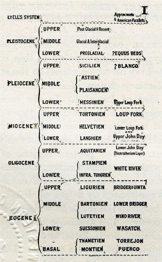
Head Progress in Earth and Planetary Science        (2021) 8:50                                                                           Page 3 of 38

 Fig. 2 Stratigraphic correlation table and orbital parameters for the last 1.9 million years, including the Early–Middle Pleistocene transition (1.4–
 0.7 Ma, Sánchez-Goñi et al. 2019; or 1.4–0.4 Ma, Head and Gibbard 2015b). The time scale is based on Fig. 1; geomagnetic polarity reversals and
 field paleointensity data are from Cohen and Gibbard (2019) and Channell et al. (2016, 2020) with ages of reversals based on orbital tuning of the
 sedimentary record (Channell et al. 2020); marine isotope record and numbering of marine isotope stages is from Lisiecki and Raymo (2005), with
 ages of terminations from Lisiecki (undated) and selected substages from Railsback et al. (2015); orbital parameters representing precession
 (Laskar et al. 2004), obliquity (Laskar et al. 2004), and eccentricity (Laskar et al. 2011) are from Head and Gibbard (2015b). Updated from Cohen
 and Gibbard (2019)

grounds that Forbes (1846) had popularized this term                         1878). By 1900, this tripartite subdivision had become
not in the sense of Lyell’s Newer Pliocene but almost                        formalized in the English literature, with Osborn using
precisely with reference to the subsequent interval of                       the terms Lower Pleistocene (preglacial), Middle Pleisto-
time for which Lyell was now introducing the term Post-                      cene (glacial and interglacial, itself subdivided into lower,
pliocene (Lyell 1863, p. 6). By 1865, Lyell had conceded                     middle and upper), and Upper Pleistocene (postglacial
that if the term Pleistocene continued to be used, then it                   and Recent) (Osborn 1900, p. 570, charts I and II)
should not be as originally intended but in place of his                     (Fig. 3).
“Post-pliocene” (Lyell 1865, footnote to p. 108). By the                       This use of subseries for the Pleistocene had become
time Lyell had unconditionally accepted the Pleistocene                      entrenched by the time of the Second International Con-
in place of his Post-pliocene (Lyell 1873, p. 3, 4), this                    ference of the Association pour l’étude du Quaternaire
suggestion had already been generally adopted, with sub-                     européen (the forerunner of the International Union for
division quickly following. The term “middle Pleisto-                        Quaternary Research [INQUA] meetings) held in Lenin-
cene” for instance was employed informally by Harkness                       grad in 1932, and subseries terms were used in a formal
as early as 1869 (Harkness 1869), and the positional                         sense by Zeuner (1935, 1945) who in 1935 was already
modifiers “early”, “middle”, and “late” have been used for                   applying Milankovitch cyclicity and insolation curves to
the Pleistocene since at least the 1870s (e.g. Dawkins                       provide absolute dates for Pleistocene successions. In
Head Progress in Earth and Planetary Science       (2021) 8:50                                                                         Page 4 of 38

 Fig. 3 Reproduction of Chart 1 of Osborn (1900), an early example of the tripartite subdivision of the Pleistocene along with other Cenozoic
 series and their subdivision. The word Pleiocene, from the Greek pleiōn (Latinized as plio-), is a rare variant spelling of Pliocene

1945, he considered the base of the Middle Pleistocene                      1963, 1964; Opdyke et al. 1966; Ninkovich et al. 1966;
to have an age of ~ 425 ka.                                                 Glass et al. 1967; see Watkins 1972 for historical review),
   The Japanese geophysicist Motonori Matsuyama (1884–                      and particularly the recognition and radiometric dating of
1958, as spelled and pronounced but mistransliterated in                    the M–B reversal and Jaramillo “event” (Doell and Dal-
his own publications and others as Matuyama) was the                        rymple 1966), that created new possibilities for global
first to document clearly from basalts in the Genbudō                       stratigraphic correlation and Pleistocene time scale cali-
(basalt caves), Japan (Matuyama 1929), the reversed mag-                    bration. Accordingly, participants at the Burg Wartenstein
netic polarity interval from 2.58 to 0.773 Ma that we now                   Symposium “Stratigraphy and Patterns of Cultural Change
call the Matuyama Reversed Polarity Chron. However, it                      in the Middle Pleistocene”, held in Austria in 1973, rec-
was the emergence of the geomagnetic polarity reversal                      ommended that “The beginning of the Middle Pleistocene
time scale for the Pleistocene in the 1960s (Cox et al.                     should be so defined as to either coincide with or be
Head Progress in Earth and Planetary Science   (2021) 8:50                                                      Page 5 of 38

closely linked to the boundary between the Matuyama Re-          Deciding upon the primary guide to the boundary
versed Epoch and the Brunhes Normal Epoch of                   should be made prior to the consideration of candidate
paleomagnetic chronology” (Butzer and Isaac 1975, ap-          sections because the expression of this guide in the
pendix 2, p. 901), as noted by Pillans (2003). In the same     GSSP must be exemplary (Remane et al. 1996). The
year, the INQUA Working Group on Major Subdivisions            Working Group’s decisions at Florence were therefore
of the Pleistocene was established at the IX INQUA Con-        crucial in moving the process forward. The M–B rever-
gress in Christchurch, New Zealand, 1973, with its pri-        sal with an age of ~ 773 ka (Singer et al. 2019; Channell
mary aim to define globally recognizable boundaries for        et al. 2020; Haneda et al. 2020a; and earlier reviews by
the lower, middle, and upper Pleistocene subseries (Rich-      Head and Gibbard 2005, 2015b) was chosen in part be-
mond 1996). The rank of subseries was adopted in prefer-       cause it (1) has an isochronous expression in most mar-
ence to stage as the latter term was already used widely in    ine and terrestrial sediments and even in ice cores, (2) is
Quaternary stratigraphy for locally and regionally defined     the most prominent geomagnetic field reversal in the
units. At the XIIth INQUA Congress in Ottawa in 1987,          past 773 kyr, and (3) occurs within the Early–Middle
the Working Group submitted a proposal, which was              Pleistocene transition (1.4–0.7 or 1.4–0.4 Ma; Fig. 2),
accepted by INQUA’s stratigraphic commission and ap-           aligning the Early–Middle Pleistocene boundary with a
proved by the congress, that “As evolutionary biostratig-      fundamental shift in Earth’s history. This shift from a 41
raphy is not able to provide boundaries that are as globally   ky to quasi-100 ky orbital rhythm was marked by in-
applicable and time-parallel as are possible by other          creases in the amplitude of climate oscillations and in
means, the Lower–Middle Pleistocene boundary should            long-term average global ice volume, and by strong
be taken provisionally at the Matuyama–Brunhes palaeo-         asymmetry in global ice volume cycles. It resulted in
magnetic reversal ...” (Anonymous 1988, p. 228; Richmond       progressive and fundamental physical, chemical, cli-
1996, p. 320). From then on, the M–B reversal became the       matic, and biotic adjustments to the planet (Head and
preferred and indeed de facto marker for the Early–Mid-        Gibbard 2015b).
dle Pleistocene boundary (e.g. Bowen 1988; Berggren et al.
1995; Pillans 2003; Gradstein et al. 2005; Head and Gib-       2.3 Voting on candidates for the Middle Pleistocene
bard 2005, 2015a, 2015b; Cita et al. 2006, 2008, Cita 2008;    Subseries GSSP
Head et al. 2008). Nonetheless, the Early–Middle Pleisto-      The three final candidates for the Early–Middle Pleisto-
cene boundary did not have official standing because this      cene GSSP were the Valle di Manche section in Calabria
required the selection and approval of a GSSP.                 and the Ideale section at Montalbano Jonico in Basili-
                                                               cata, both in Italy, and the Chiba section in Japan (Head
2.2 Selecting a primary guide for the base of the Middle       and Gibbard 2015a) (Fig. 4). Following field trips that
Pleistocene Subseries                                          allowed members of the Working Group to visit all three
The XIVth INQUA Congress in Berlin in 1995 focused             sites in advance of voting (Ciaranfi et al. 2015; Okada
on three potential candidate GSSPs: Chiba in Japan,            and Suganuma 2018), the vigorous and exhaustive
Montalbano Jonico in Basilicata, Italy, and the Wanganui       process of selecting a GSSP began on July 11, 2017, with
Basin in New Zealand (Pillans 2003), the latter being dis-     the circulation of proposals to the membership of the
counted because it contained unconformities (Head              Working Group (Table 1). It had been decided by all
et al. 2008). Meanwhile, the ICS Subcommission on              three proponents in advance that the proposals should
Quaternary Stratigraphy (SQS), in 2002 after a period of       remain confidential because they contained unpublished
inactivity, established a Working Group to review all as-      material. This confidentiality was respected through the
pects of the Early–Middle Pleistocene boundary includ-         entire selection process. Discussions started on July 25
ing the selection of a suitable GSSP (Head et al. 2008).       and ended at the close of October 3, 2017, allowing an
At the 32nd International Geological Congress in Flor-         extended opportunity to exchange views. Discussions
ence in 2004, the Early–Middle Pleistocene boundary            were wide-ranging, in acknowledgement that a GSSP
Working Group recommended that (1) The boundary be             must record an array of stratigraphic markers, but inev-
defined in a marine section at a point “close to” the          itably focused on the M–B reversal. A detailed commen-
Matuyama–Brunhes palaeomagnetic reversal, where the            tary on these discussions is given in Head (2019) and
definition of “close” was agreed to mean within plus or        only key aspects will be presented here.
minus one isotope stage of the reversal; and (2) the              The M–B reversal in the Chiba composite section (CbCS)
GSSP should be located in a marine section exposed on          is expressed by directional changes (virtual geomagnetic pole
land, not in a deep sea core (Head et al. 2008). A third       [VGP] latitudes) and changes in the geomagnetic field inten-
potential candidate GSSP emerged at the Florence con-          sity based on both the paleomagnetic record and a coherent
gress: the Valle di Manche section in Calabria, Italy          record of its proxy, the authigenic 10Be/9Be record (Suga-
(Capraro et al. 2004, 2005) (Fig. 4).                          numa et al. 2015; Okada et al. 2017; Simon et al. 2019;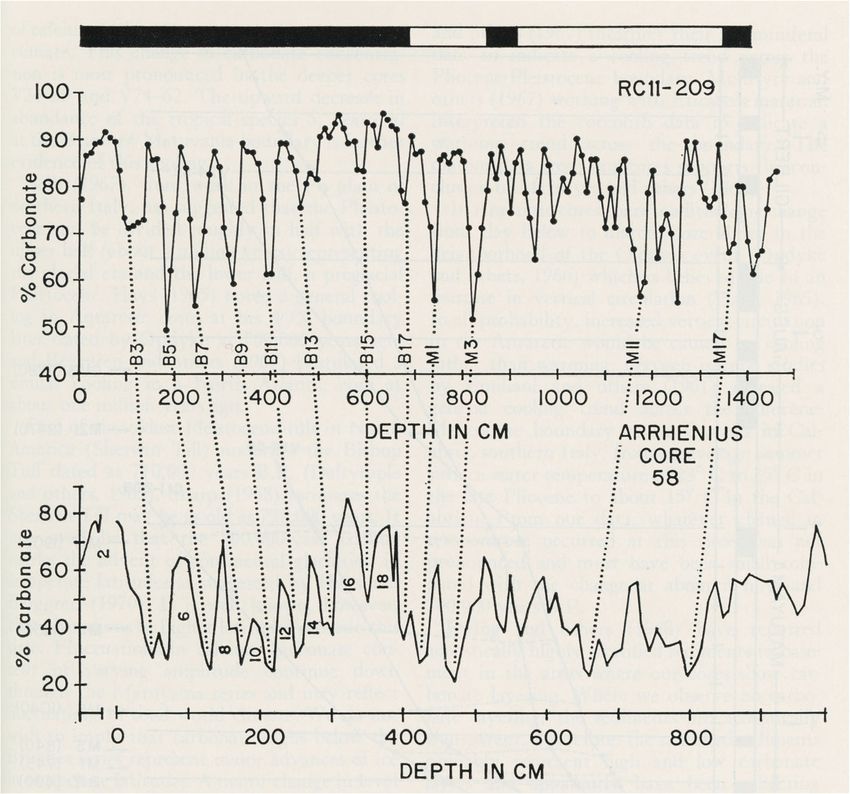
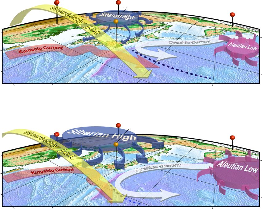
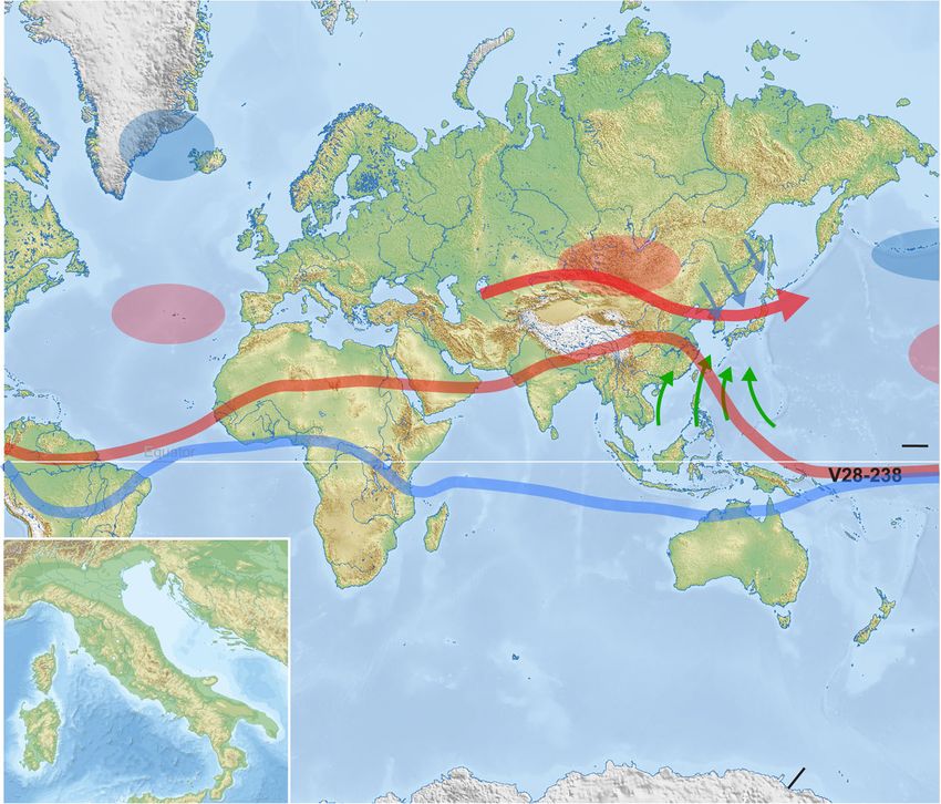
Head Progress in Earth and Planetary Science           (2021) 8:50                                                                                Page 6 of 38

 Fig. 4 Location of sites discussed in the text and present atmospheric features. ODP Site 983 Gardar Drift, Iceland Basin; IODP Site U1313 upper western
 flank of the Mid-Atlantic Ridge, central North Atlantic; IODP Site U1385 southwest Portuguese margin; ODP Site 976 Alboran Sea; ODP Site 975 western
 Mediterranean Sea; Core KC01B Ionian Sea; Core MD900963 tropical Indian Ocean; Lake Baikal, SE Siberia; Yimaguan and Luochuan, Chinese Loess
 Plateau; Chiba composite section, Japan; Vema 28-238 and RC11-209 cores, western equatorial Pacific Ocean; ODP Site 1123 Chatham Ridge, South
 Pacific; EPICA Dome C ice core (75° 06′ S, 123° 21′ E, location is off the map); Core 58 of Arrhenius (1952), eastern equatorial Pacific Ocean (6° 44′ N, 129°
 28′ W; location is off the map); inset shows important Italian sites. The Westerly Jet (WJ) during summer (S), East Asian Summer/Winter Monsoon (EASM/
 EAWM), and summer/winter variation in the position of the Intertropical Convergence Zone (ITCZ) adapted from Cheng et al. (2012) and Liu et al.
 (2015); the Siberian High (SH) and Aleutian Low (AL) are primarily winter atmospheric pressure systems; the AL and Pacific High (PH) form the North
 Pacific Oscillation; the Islandic Low (IL) and Azores High (AH) form the North Atlantic Oscillation

Haneda et al. 2020a). These studies are based on an astro-                        reversal is 772.9 ± 5.4 ka, with a duration of up to ~ 2 kyr.
nomical age model introduced by Suganuma et al. (2015)                            The close match between the geomagnetic field intensity and
and refined by Okada et al. (2017) and again by Suganuma                          the 10Be/9Be record confirms that any lock-in depth offset
et al. (2018). Okada et al. (2017) determined the directional                     (Roberts and Winklhofer 2004; Suganuma et al. 2010, 2011)
midpoint at 771.7 ka with a duration of 2.8 kyr; these values                     at this high sedimentation rate site (89 cm/kyr across the
revised to 772.9 ka and 1.9 kyr on the age model of Suga-                         boundary) is minimal. This age closely accords with ages of
numa et al. (2018). Simon et al. (2019) using new                                 around 773 ka from other well constrained sites
paleomagnetic data reported a directional switch between                          (Channell 2017; Channell et al. 2020; Singer et al.
773.9 and 771.9 ka, with a duration therefore of 2.0 kyr.                         2019; Valet et al. 2019; Haneda et al. 2020a; earlier
Haneda et al. (2020a) using new paleomagnetic data com-                           records reviewed in Head and Gibbard 2015b). The
bined with earlier studies (Suganuma et al. 2015; Hyodo                           geomagnetic field intensity record shows two pro-
et al. 2016; Okada et al. 2017) determined the average direc-                     nounced minima, one at 772 ka near the polarity
tional midpoint at 772.9 ka with a duration of 1.1 kyr based                      switch and the other at 764 ka (Simon et al. 2019). It
on the age model of Suganuma et al. (2018). Allowing for a 5                      is therefore evident that the position of the VGP
kyr chronological uncertainty in the orbital tuning of the                        switch cannot be precisely predicted using geomag-
CbCS (4 kyr from Lisiecki and Raymo 2005, and 1 kyr from                          netic field intensity data alone.
Elderfield et al. 2012; see Suganuma et al. in press) and a                         Montalbano Jonico lacks a paleomagnetic record
stratigraphic uncertainty of 0.4 ka (Haneda et al., 2020a), the                   owing to late diagenetic remagnetization associated with
astronomical age of the directional midpoint of the M–B                           the growth of greigite (Sagnotti et al. 2010). A 10Be/9Be
Head Progress in Earth and Planetary Science           (2021) 8:50                                                             Page 7 of 38

Table 1 Members of the SQS Working Group on the Early–                        when compared with most global records including the
                                                                              10
Middle Pleistocene Boundary in 2017 at the time of voting on                     Be/9Be proxy record of Montalbano Jonico section just
the GSSP                                                                      135 km to the north (Head 2019). A 10Be/9Be record at
• Luca Capraro, Dipartimento di Geoscienze, Università degli Studi di         the Valle di Manche section gives a peak in 10Be concen-
  Padova, Padova, Italy
                                                                              tration ∼3.5 m above the reported M–B reversal. This
• Bradford M. Clement, Integrated Ocean Drilling Program and                  translates to a difference of ∼12 kyr (Capraro et al. 2018)
  Department of Geology and Geophysics, Texas A&M University, College
  Station, USA                                                                and is coincident with the age of this reversal elsewhere.
                                                                              Lock-in depth seems unable to explain the spuriously
• Mauro Coltorti, Dipartimento di Scienze Fisiche, della Terra e
  dell’Ambiente, Università di Siena, Siena, Italy                            low position of the reversal because sedimentation rates
• Craig S. Feibel, Department of Earth and Planetary Sciences, Rutgers
                                                                              at ∼27 cm/kyr in this part of the Valle di Manche section
  University, Piscataway, New Jersey, USA                                     are reasonably high (Macrì et al. 2018). When the
                                                                              10
• Martin J. Head, Department of Earth Sciences, Brock University, St.            Be/9Be curves for the Valle di Manche and Montal-
  Catharines, Ontario, Canada (Co-Convener)                                   bano Jonico sections are compared, they show strong
• Lorraine E. Lisiecki, Department of Earth Science, University of            agreement (Capraro et al. 2019). The 10Be/9Be peak
  California, Santa Barbara, USA                                              therefore most likely marks the true position of the M–
• Jiaqi Liu, Institute of Geology and Geophysics, Chinese Academy of          B Chron boundary at both sections, with the Valle di
  Sciences, Beijing, China                                                    Manche paleomagnetic reversal ∼3.5 m below represent-
• Maria Marino, Dipartimento di Scienze della Terra e Geoambientali,          ing diagenetic overprinting and remagnetization (Head
  Università degli Studi di Bari Aldo Moro, Bari, Italy                       2019; but see Capraro et al. 2019 for an alternative inter-
• Anastasia K. Markova, Institute of Geography, Russian Academy of            pretation). This explanation would also account for the
  Sciences, Moscow, Russia                                                    unusually rapid directional transition of this reversal in
• Brad Pillans, Research School of Earth Sciences, Australian National        the order of 100 years or less at the Valle di Manche
  University, Canberra, ACT, Australia (Co-Convener)
                                                                              section (Macrì et al. 2018). A similar relatively old (786.1
• Yoshiki Saito, Geological Survey of Japan, AIST, Tsukuba, Ibaraki, Japan;   ± 1.5 ka) M–B reversal, perhaps with an even more rapid
  and Estuary Research Center, Shimane University, Matsue, Shimane,
  Japan                                                                       transition, reported from the Sulmona basin in central
                                                                              Italy (Sagnotti et al. 2014; Sagnotti et al. 2016) has been
• Brad S. Singer, Department of Geoscience, University of Wisconsin–
  Madison, USA                                                                restudied and appears to carry an unreliable signal (Ev-
• Yusuke Suganuma, National Institute of Polar Research, Tachikawa,
                                                                              ans and Muxworthy 2018; but see Sagnotti et al. 2018).
  Tokyo, Japan and Department of Polar Science, School of                     Another relatively old age (~ 779 ka) for the reversal has
  Multidisciplinary Sciences, The Graduate University for Advanced            been reported from Site IODP U1385 off Portugal (Sán-
  Studies (SOKENDAI), Tachikawa, Tokyo, Japan
                                                                              chez-Goñi et al. 2016). The position of this reversal has
• Charles Turner, Department of Earth Sciences, The Open University,          since been revised, and it is now provisionally placed
  Milton Keynes, UK
                                                                              higher in the core than reported from shipboard analysis
• Chronis Tzedakis, Department of Geography, University College               (Xuan Chuang, pers. comm. 2018). Moreover, a reported
  London, London, UK
                                                                              M–B reversal age of 783.4 ± 0.6 ka at ODP Site 758 in
• Thijs van Kolfschoten, Faculty of Archaeology, Leiden University,
  Leiden, The Netherlands
                                                                              the Indian Ocean (Mark et al. 2017) has been challenged
                                                                              on grounds that the sedimentation rates and hence reso-
                                                                              lution of the isotope and magnetic stratigraphies are all
                                                                              too low for precise age determination (Channell and
record at this site serves as a proxy for the geomagnetic                     Hodell 2017).
field intensity site and reveals a peak (field intensity                         It had been decided in advance that the choice individ-
minimum) at the approximate position of the M–B re-                           ual members made when voting within the Working
versal as determined by the marine isotope record (Si-                        Group would not be revealed, contrary to usual practice
mon et al. 2017; Nomade et al. 2019) and dated by an                          within ICS. Because of active and potential research col-
40
   Ar/39Ar age of 774.1 ± 0.9 ka for tephra layer V4 which                    laborations within the group, to do otherwise might have
coincides with the 10Be/9Be peak (Nomade et al. 2019).                        compromised the vote. Voting by the SQS Working
While this corroborates the position and age of the M–B                       Group commenced on October 10, 2017, and concluded
reversal in this part of the Mediterranean, the geomag-                       on November 10, 2017. As noted in Head (2019), the
netic field intensity alone is insufficient to identify the                   Chiba proposal was passed by supermajority, gaining
precise position of the polarity switch (see Channell et al.                  73% of the total votes cast.
2020), as demonstrated for Chiba and elsewhere.
   The M–B reversal as recorded at the Valle di Manche                        2.4 Final approval and ratification of the Chiba GSSP
(Capraro et al. 2017) has been astronomically dated at                        Following minor revision, the Chiba proposal was submit-
786.9 ± 5 ka (Macrì et al. 2018), an anomalously old age                      ted to the SQS voting membership for discussion and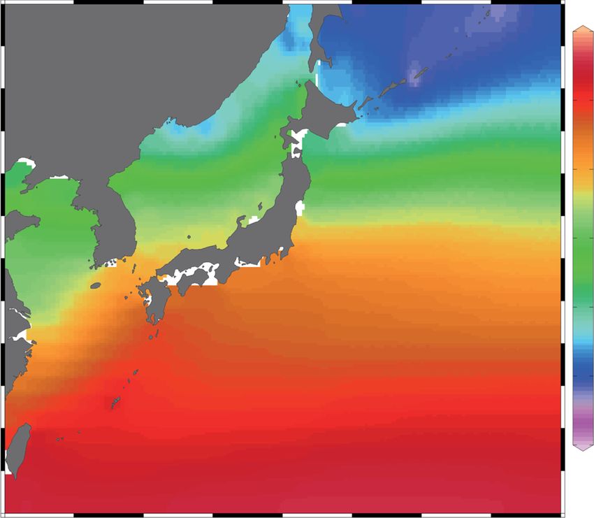
Head Progress in Earth and Planetary Science (2021) 8:50 Page 8 of 38
voting, this process concluding on 16 November 2018 3.1 History of MIS 19
with a supermajority of 86% in favour of the Chiba pro- In labelling fluctuating percentages of carbonate in mar-
posal. Discussion within the ICS voting membership ine cores from the equatorial Pacific Ocean, Arrhenius
began on August 16, 2019, and closed on October 28, (1952) introduced a numbering system in which even/
2019. Voting concluded on November 28, 2019, with the odd numbers represent glacial/interglacial cycles. Arrhe-
results as follows: 17 in favour, 2 against, no abstentions, nius correctly surmised that carbonate-rich layers repre-
all ballots returned. The proposal was therefore carried sent increased productivity linked to upwelling driven by
with a supermajority of 89.5%. This ICS-approved pro- strengthened trade winds during glacial intervals. Arrhe-
posal for the Chibanian Stage/Age and Middle Pleistocene nius labelled 18 carbonate cycles, recording although not
Subseries/Subepoch was ratified in full by the IUGS EC labelling older cycles including the equivalent of what
on January 17, 2020, drawing to a close a process initiated was to be known as MIS 19 (Fig. 5). Hays et al. (1969)
by INQUA in 1973, some 47 years earlier. continued this research through additional cores in the
The GSSP is placed at the base of a regional lithostra- Pacific. They labelled as B17 (where B = Brunhes) a
tigraphic marker, the Ontake-Byakubi-E (Byk-E) tephra carbonate-poor interglacial cycle coinciding with the
bed (Takeshita et al. 2016), in the Chiba section. It has base of the Brunhes Chron (Fig. 5). Emiliani’s (1955,
an astronomical age of 774.1 ka (Suganuma et al. in 1966) original oxygen isotope stages followed the num-
press) and a zircon U-Pb age of 772.7 ± 7.2 ka (Suga- bering scheme of Arrhenius. Shackleton and Opdyke
numa et al. 2015), occurring immediately below the top (1973) in their now famous oxygen isotope and magne-
of Marine Isotope Substage 19c. The directional mid- tostratigraphic analysis of the Vema 28-238 core from
point of the M–B reversal, serving as the primary guide the western equatorial Pacific Ocean (V28-238 in Fig. 4)
to the boundary, is just 1.1 m above the GSSP and has extended to Stage 22 Emiliani’s original oxygen isotope
an astronomical age of 772.9 ± 5.4 ka (Haneda et al. stages 1–14 (Emiliani 1955) and then 1–17 (Emiliani
2020a; Suganuma et al. in press). The numerous clima- 1966). In doing so, Shackleton and Opdyke (1973) were
tostratigraphic signals associated with the MIS 19c/b the first to label MIS 19 (Fig. 6). They equated cycle B17
transition, which represents the inception of glaciation of Hays et al. (1969) with their MIS 19, confirming the
for MIS 19 (see below), provide additional means to association of this interglacial stage with the M–B
identify this boundary precisely on a global scale. reversal.
IUGS ratification of the Middle Pleistocene Subseries of-
ficially legitimized a unit-rank term already in wide and
formal use within the Quaternary community (Head et al. 3.2 Subdivision of MIS 19
2017), and the ratification of an accompanying stage com- The division of marine isotope stages into substages has
plied with the requirements of the International Commis- a long history beginning with Shackleton (1969) who
sion on Stratigraphy. INQUA fully supported ratification subdivided MIS 5 into five lettered substages, a–e (Rails-
of both stage and subseries (van Kolfschoten 2020). This back et al. 2015). As noted by Railsback et al. (2015), a
also provided Japan with its first GSSP, coincidentally parallel system of subdividing marine isotope stages into
based on a paleomagnetic reversal first clearly docu- decimal-style numbered “events” has its roots in the la-
mented in Japan by Motonori Matsuyama, an early Japa- belling system of Arrhenius (1952) and was first applied
nese pioneer of magnetostratigraphy. The achievements of to marine isotope stages by Prell et al. (1986; but see
Japanese geophysicist Naoto Kawai may also be recalled, Railsback et al. 2015 for historical development) who
as he was the first to record a paleomagnetic reversal in reasoned that defining events (peaks and troughs) rather
sedimentary rocks (Kawai 1951). than stages (intervals of sediment or time) was more
useful in applying tie points for age models. Although
the two approaches tended to be used rather indiscrim-
3 Marine Isotope Stage 19 inately and interchangeably, Shackleton (2006) remarked
MIS 19 has long been associated with the M–B reversal, that conceptually they are different and not interchange-
and this interglacial stage therefore provides a well- able. He noted that “events” relied upon peak values in
documented cluster of additional stratigraphic signals to analyses that are more difficult to replicate in practice,
identify the base of the Chibanian Stage on a global and hence reliably correlate, than the midpoints of tran-
scale. Its climatic evolution is also significant because sitions that define substage boundaries. This midpoint
MIS 19c serves as an orbital analogue for the present approach is indeed is how stages themselves are defined
interglacial (e.g. Berger and Loutre 1991; Pol et al. 2010; following Emiliani (1955). Accordingly, Shackleton
Tzedakis et al. 2012a, 2012b; Yin and Berger 2015) and (2006), Railsback et al. (2015) in their extensive review,
therefore provides a natural baseline for assessing our and the present study, have all favoured contiguous let-
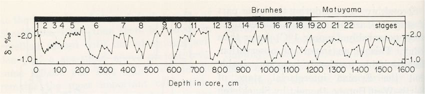
future climate. tered subdivisions for marine isotope stages.Head Progress in Earth and Planetary Science (2021) 8:50 Page 9 of 38 Fig. 5 Reproduction of fig. 14 in Hays et al. (1969) showing correlation between carbonate percentage in equatorial Pacific core RC11-209 and that of east equatorial Pacific core 58 of Arrhenius (1952). Carbonate cycle B17 in core RC11-209 corresponds to an unlabelled cycle in Arrhenius’ core 58. This would have been cycle 19 had Arrhenius continued labelling. Cycle B17 aligns with the Matuyama–Brunhes paleomagnetic reversal and represents MIS 19 3.2.1 Subdivision used in the present study MIS 19c, terminating with a glacial inception (Tzedakis The scheme used here is illustrated by its application to et al. 2012a, 2012b). MIS 19b represents a single interval the CbCS record (Fig. 7). Three substages, 19c, 19b, and of heavier foraminiferal isotopic values (Nomade et al. 19a, are recognized. MIS 19c comprises full interglacial 2019) which is recognized at the CbCS within the ben- conditions together with the rise to lighter foraminiferal thic record (Haneda et al. 2020b). The benthic foraminif- δ18O values at the beginning of MIS 19 (Termination eral δ18O record of MIS 19a is represented by a series of IX) and the decline to heavier values towards the end of millennial-scale oscillations, with as many as four peaks Fig. 6 Reproduction of fig. 9 in Shackleton and Opdyke (1973) showing the δ18O record of the planktonic foraminifera Globigerinoides sacculifera from core V28-238, western equatorial Pacific, from which MIS 19 was defined for the first time (Shackleton and Opdyke 1973). This study confirms the links between MIS 19, carbonate cycle B17 of Hays et al. (1969), and the Matuyama–Brunhes paleomagnetic reversal
Head Progress in Earth and Planetary Science         (2021) 8:50                                                                          Page 10 of 38

 Fig. 7 Differing subdivisions of the interval comprising Marine Isotope Substages 19b and 19a illustrated using the isotope record of the Chiba
 composite section (CbCS; Haneda et al. 2020b). (a) Four millennial-scale benthic isotope oscillations (MIS 19a-o1 to MIS 19a-o4) represented in the
 benthic foraminiferal record by lighter values exclusively within MIS 19a. Four stadials (MIS 19-s1 to MIS 19-s4) and four interstadials (MIS 19-i1 to
 MIS 19-i4) reflect more localized millennial-scale paleoenvironmental alternations across MIS 19b–a, in this case characterized by the planktonic
 foraminiferal record. (b) The labelling scheme of Haneda et al. (2020b) based on the planktonic foraminiferal record of the CbCS. (c) The labelling
 scheme of Nomade et al. (2019) based on the benthic foraminiferal record of Montalbano Jonico, Italy

of lighter isotopic values here labelled as MIS 19a-o1 to                     the basis of two pronounced planktonic foraminiferal
MIS 19a-o4, where “o” refers to benthic isotope oscilla-                      δ18O peaks recorded from Core MD900963 in the trop-
tion. MIS 19a begins with MIS 19a-o1 (Fig. 7).                                ical Indian Ocean (Fig. 4). No explanation was given for
  Superimposed on this benthic foraminiferal isotopic                         these two peaks although precession is strongly
record through MIS 19b–a is as many as four stadial–                          expressed in this core.
interstadial alternations, here labelled MIS 19-s1 to MIS                       Tzedakis et al. (2012a, 2012b) seem to have initiated
19-s4 (stadials) and MIS 19-i1 to MIS 19-i4 (intersta-                        the application of lettered substages for MIS 19, with
dials). MIS 19-s1 is the first of these millennial-scale cli-                 Tzedakis et al. (2012b, their fig. 4) applying MIS 19a,
matic episodes and broadly coincides with the glacial                         19b, and 19c to the foraminiferal δ18O and ice-rafted
inception marked by MIS 19b. They are recognized pri-                         debris (IRD) record from ODP Site 983 on the Gardar
marily in planktonic records including planktonic fora-                       Drift, North Atlantic (Figs. 4 and 8c) and correlating this
miniferal δ18O, but may be observed in pollen spectra                         to the Antarctic ice-core record of EPICA Dome C
and other terrestrial proxies.                                                (Figs. 4 and 8c). Tzedakis et al. (2012b) did not define
  Figure 7 shows how the labelling scheme presented here                      the boundaries of their substages but MIS 19c clearly
differs from those of Nomade et al. (2019) and Haneda et al.                  represents the rise to lightest isotopic values and the en-
(2020b) as applied to the isotopic record of the CbCS. The                    suing peak or plateau followed by a gradual decline to
present scheme does not preclude the use of additional bio-                   heavier values in the upper part of MIS 19c. MIS 19b
zones and informal event stratigraphy through all or part of                  and MIS 19a together represent three succeeding peaks
MIS 19 where such detail is needed. The rationale for this                    of light isotopic values, here labelled interstadials i1, i2,
subdivision is discussed in Section 3.2.3.                                    and i3, that characterize the upper part of MIS 19. MIS
                                                                              19b includes the two lowest interstadials and MIS 19a
3.2.2 Division into substages                                                 includes the third. Tzedakis et al. (2012b) correlated
Bassinot et al. (1994) were the first to subdivide MIS 19                     these three interstadials in the upper part of MIS 19
formally, defining MIS 19.1, 19.2, and 19.3 (Fig. 8b) on                      at Site 983 with three Antarctic Isotope Maxima
Head Progress in Earth and Planetary Science (2021) 8:50 Page 11 of 38 Fig. 8 North Atlantic and global records of Marine Isotope Stage 19 (see also Fig. 9). (a) Insolation at 65° N in June, and precession and obliquity parameters. (b) Designation of events by Bassinot et al. (1994) based on the planktonic foraminiferal δ18O record of Indian Ocean core MD900963. (c) Lettered substages of Tzedakis et al. (2012b) applied to the foraminiferal δ18O and other records of ODP Site 983 Iceland Basin, with peaks correlated to Antarctic Isotope Maxima (AIMs) reflected in the Antarctic ice-core methane record from EPICA Dome C. Also included are the ice-rafted debris and sortable silt mean size (mean of 10– 63 μm fraction) records (Kleiven et al. 2011). (d) Lettered substages of Railsback et al. (2015) as applied to the LR04 benthic δ18O foraminiferal stack of Lisiecki and Raymo (2005). (e) The MIS 19 subdivisional scheme used here (Fig. 7): interstadials i1, i2, and i3 are labelled in red. All records are plotted on their own published time scales and use the original substage designations
Head Progress in Earth and Planetary Science          (2021) 8:50                                                                           Page 12 of 38

(AIMs) documented in the EPICA Dome C ice-core                                 Railsback et al. (2015) assigned both peaks to MIS
record (EPICA Community Members 2006). Hence,                                  19a and the preceding trough to MIS 19b (Fig. 8d).
the two lowest interstadials, assigned to MIS 19b,                             This scheme therefore differed significantly from that
were correlated to AIM C and B, and the uppermost                              of Tzedakis et al. (2012b).
interstadial, assigned to MIS 19a, was correlated to                             Ferretti et al. (2015) published detailed benthic and
AIM A (Fig. 8c).                                                               planktonic foraminiferal δ18O records from IODP
  Railsback et al. (2015) similarly subdivided MIS 19                          Site U1313 in the central North Atlantic (Fig. 4), al-
into substages a, b, and c, but defined them with re-                          though the upper part of MIS 19 could not be un-
spect to the LR04 global benthic foraminiferal δ18O                            ambiguously resolved into three interstadials. MIS
stack of Lisiecki and Raymo (2005) which only clearly                          19c and MIS 19a were therefore labelled only ap-
distinguishes two peaks in the upper part of MIS 19.                           proximately and MIS 19b was omitted (Fig. 9b).

 Fig. 9 North Atlantic records of Marine Isotope Stage 19 (see also Fig. 8). (a) Insolation at Equator in spring and autumn, and absolute maximum
 of mean irradiance (Laskar et al. 2004; Ferretti et al. 2015; Haneda et al. 2020b). (b) IODP Site U1313 central North Atlantic: foraminiferal δ18O
 (Ferretti et al. 2015). (c) IODP Site U1385 southwest Portuguese margin: foraminiferal δ18O, alkenones (C37:4), and pollen records with grey bars
 indicating major contractions of the Mediterranean forest; the Tajo Interglacial occurs within MIS 19c, and a dark blue triangle marks a brief
 cooling event just before it (Sánchez-Goñi et al. 2016); stadials (s1–s3) and interstadials (i1–i3) are labelled following the correlations of Regattieri
 et al. (2019) and Nomade et al. (2019). (d) The MIS 19 subdivisional scheme used here (Fig. 7). All records are plotted on their own published time
 scales and use the original substage designations
Head Progress in Earth and Planetary Science   (2021) 8:50                                                       Page 13 of 38

   Sánchez-Goñi et al. (2016) in their study of IODP Site           The Ideale section of Montalbano Jonico, Basilicata,
U1385 off southwest Portugal (Fig. 4) extended the               Italy (Fig. 4), yields one of the most detailed δ18O re-
upper boundary of MIS 19c to the top of the plateau of           cords of MIS 19 available (Simon et al. 2017; Nomade
lightest δ18O values. The progressive decline to heavier         et al. 2019). MIS 19b is restricted to a brief cooling event
values as well as the first of three conspicuous peaks in        following MIS 19c, and MIS 19a includes discrete inter-
the upper part of MIS 19 were assigned to MIS 19b. The           vals of lighter isotopic values labelled by Nomade et al.
second and third peaks were assigned to MIS 19a                  (2019) as interstadials 1 through 3, with a fourth labelled
(Fig. 9c). This scheme essentially follows that of Tzeda-        in the present study (fig. 8b in Nomade et al. 2019;
kis et al. (2012b). Sánchez-Goñi et al. (2016) determined        Fig. 10d).
the MIS 20/19 and MIS 19/18 boundaries at the mid-                  A somewhat truncated planktonic foraminiferal
points between highest/lowest and lowest/highest values          δ18O record of ODP Site 976, Alboran Sea, western
in the δ18O benthic foraminiferal record, an approach            Mediterranean (Toti et al. 2020; Fig. 4) does not dis-
following that of Shackleton et al. (2003) for establishing      tinguish between MIS 19b and MIS 19a, although two
the MIS 6/5e and MIS 5e/d boundaries. They then ap-              interstadials and the onset of a third in the upper
plied the same method to determine the positions of the          part of MIS 19 can be referred to interstadials i1–i3
MIS 19c/b and MIS 19b/a boundaries, finding that the             (Fig. 10e).
midpoints were broadly similar to positions they had sta-           The highly resolved δ18O record from the CbCS, Japan
tistically identified by the “Change point method” of Zei-       (Haneda et al. 2020b; Suganuma et al. in press; Fig. 4),
leis et al. (2002, 2003). Therefore, these limits and the        has been subdivided into lettered substages such that
substage classification they embody may reflect signifi-         four peaks identified in the upper part of MIS 19 are all
cant changes in global ice volume (Sánchez-Goñi et al.           assigned to MIS 19a (Fig. 11). This scheme follows the
2016). This method does not appear to have been used             classification of Nomade et al. (2019).
on other foraminiferal benthic records of MIS 19 to test            It is evident from the foregoing that most records of
such a possibility, but the shape of the δ18O benthic fo-        MIS 19 naturally allow subdivision into two parts, an
raminiferal record at the CbCS in Japan (Fig. 7), for ex-        earlier relatively stable phase representing MIS 19c and
ample, is rather different from that at Site U1385               occurring within one precession cycle, and a later phase
especially across the MIS 19b–a interval.                        (the inconsistently applied MIS 19b and MIS 19a) usu-
   Regattieri et al. (2019) in their study of the lacustrine     ally featuring three or four millennial-scale isotopically
Sulmona basin in central Italy (Figs. 4 and 10b) broadly         light peaks and occurring within a second precession
followed the lettered substage classification of Sánchez-        cycle. There might be merit in dividing MIS 19 into just
Goñi et al. (2016). Their MIS 19b, the base of which is          two substages separated by the current MIS 19c/b
placed between two reduced-precipitation events (V and           boundary as this most reasonably represents the incep-
VI), includes stadial s1, interstadial i1 and part of the fol-   tion of glaciation (Tzedakis et al. 2012a), and indeed
lowing stadial, s2. The MIS 19b–a boundary is drawn              Nomade et al. (2019) considered MIS 19b as the first bi-
midway through their event IIX, here labelled stadial s2.        polar seesaw oscillation. However, the tripartite subdiv-
In total, three interstadials are recognized within the          ision first introduced by Bassinot et al. (1994) has
MIS 19b–a interval at Sulmona (Fig. 10b), as with IODP           become entrenched. The approach used here is therefore
Site U1385.                                                      to follow the substage classification of Nomade et al.
   The lacustrine Piànico-Sèllere basin of northern              (2019) and Haneda et al. (2020b) in which MIS 19b is
Italy (Fig. 4) contains a finely resolved pollen record          restricted to the first interval of high benthic isotopic
established by Moscariello et al. (2000). Although pre-          values following MIS 19c.
viously assigned to MIS 11, it most likely represents
MIS 19 based on tephrochronology (Pinti et al. 2001,             3.2.3 Fine-scale subdivision of MIS 19
2007; Roulleau et al. 2009) and paleoclimatic concord-           Millennial to centennial changes occurring within
ance with other Italian sites (Nomade et al. 2019).              MIS 19 include both local and global signals. Recog-
Nomade et al. (2019) labelled the Piànico-Sèllere                nizing events, for example of warming or drying, and
pollen record (Fig. 10c) following their new classifica-         numbering them consecutively without reference to
tion of the Ideale section of Montalbano Jonico which            their substage is the simplest approach. Sánchez-Goñi
recognizes at least three interstadials for MIS 19a and          et al. (2016) applied constrained cluster analysis to
restricts MIS 19b to a single stadial, here labelled s1.         subdivide their pollen record of Site U1385 into 20
Although based on pollen percentages, the record of              numbered pollen biozones through MIS 19, and then
the Piànico-Sèllere basin allows precise comparison              used the relative abundances of Mediterranean pollen
with the marine isotope substages and recognition of             taxa to indicate intervals of Mediterranean forest con-
at least interstadials i1 and i2 in MIS 19a.                     traction (Fig. 9c). Regattieri et al. (2019) in their study
Head Progress in Earth and Planetary Science           (2021) 8:50                                                                             Page 14 of 38

 Fig. 10 Mediterranean records of Marine Isotope Stage 19. (a) Insolation at Equator in spring and autumn, and absolute maximum of mean irradiance
 (Laskar et al. 2004; Ferretti et al. 2015; Haneda et al. 2020b). (b) Lacustrine Sulmona basin, central Italy: endogenic calcite δ18O, events I–IX of reduced
 precipitation based on δ18O, and tephra beds (positions based on modelled ages with 40Ar/39Ar ages shown separately) used to construct the age
 model, all from Regattieri et al. (2019); Younger Dryas-like event (YDt) from Giaccio et al. (2015). (c) Lacustrine Piànico-Sèllere basin, northern Italy:
 pollen (Nomade et al. 2019). (d) Ideale section, Montalbano Jonico, Italy: benthic foraminiferal δ18O and supporting age control using 40Ar/39Ar-dated
 tephra (volcaniclastic) beds V3 and V4 from Nomade et al. (2019). Ghost sapropel assigned to insolation cycle 74, alkenone sea-surface temperature
 (SST) with Heinrich-type (Med-HTIX) Mediterranean Bølling-Allerød-type (Med-BATIX), and Younger-Dryas-type (Med-YDTIX) episodes associated with
 Termination IX, and total coccolith abundance and mesothermic arboreal pollen records showing phases I–III of climatic amelioration; from Marino
 et al. (2020). (e) ODP Site 976 Alboran Sea, western Mediterranean: planktonic foraminiferal δ18O and pollen (first component of Principal Component
 Analysis); light blue triangles show temperate forest contractions within MIS 19c and correspond to increases in total coccolithophore abundance; dark
 blue triangle represents a climate event marked by abundant Asteraceae pollen (Toti et al. 2020). The subdivisional scheme of Nomade et al. (2019) is
 given. (f) The MIS 19 subdivisional scheme used here (Fig. 7): benthic marine isotope oscillations o1–o4 are labelled in red, interstadials i1–i4 are
 labelled in red and orange. All records are plotted on their own published time scales and use the original substage designations
Head Progress in Earth and Planetary Science              (2021) 8:50                                                                                  Page 15 of 38

 Fig. 11 Chiba composite section (CbCS), Japan; records of Marine Isotope Stage 19 based on the age model of Suganuma et al. (2018). (a) Insolation
 at Equator in spring and autumn, and absolute maximum of mean irradiance (Laskar et al. 2004; Ferretti et al. 2015; Haneda et al. 2020b). (b) Total
 organic carbon wt.% (Izumi et al. 2021). (c) Percentage abundance of Protoceratium reticulatum cysts and total dinoflagellate cyst concentrations
 interpreted as a southward shift of the Kuroshio Extension during stadial s1 and early interstadial i1 (Balota et al. 2021). (d) Percentage abundance of
 calcareous nannofossil Florisphaera profunda, an indicator of near-surface ocean stratification (Kameo et al. 2020). (e) Profile of ΔT (δ18Obenthic minus
 δ18OGlobigerina bulloides) as a measure of the vertical temperature gradient between surface and bottom waters (thin grey line) and 1000-year moving
 average (thicker black line) (Haneda et al. 2020b, 2020c). (f) Profile of Δδ18Oinf-bul (δ18OGloborotalia inflata minus δ18OGlobigerina bulloides) as an indicator of
 near-surface ocean stratification (Kubota et al. 2021). (g) Planktonic and benthic foraminiferal δ18O records (Haneda et al. 2020b). (h) The MIS 19
 subdivisional scheme used here (Fig. 7): benthic marine isotope oscillations o1–o4 and interstadials i1–i4 are labelled in red, stadials s1–s4 are labelled
 in blue. (i) Substage classification and interstadial and stadial classification and labelling of Haneda et al. (2020b) where MIO = Millennial Isotopic
 Oscillation, showing MIO-Stadial 1 to 4 (MIO-S1 to MIO-S4), and MIO-Interstadial 1 to 4 (MIO-I1 to MIO-I4); YDt = Younger Dryas-type cooling subevent
Head Progress in Earth and Planetary Science   (2021) 8:50                                                      Page 16 of 38

of the lacustrine Sulmona basin in Italy recognized               The labelling scheme proposed here (Section 3.2.1;
nine events of reduced precipitation inferred from              Fig. 7) extends and modifies the schemes of Nomade
multiple paleoenvironmental proxies. These events               et al. (2019) and Haneda et al. (2020b). It treats separ-
were labelled I–IX and occur throughout MIS 19                  ately the benthic isotopic record in which as many as
(Fig. 10b).                                                     four millennial-scale oscillations (MIS 19a-o1 to MIS
   An additional approach is the recognition of numbered        19a-o4) may be discerned, and the planktonic / terres-
stadials and interstadials. These have been used tradition-     trial record in which as many as four stadials (MIS 19-s1
ally to describe cooler and warmer episodes within glacial      to MIS 19-s4) and four interstadials (MIS 19-i1 to MIS
cycles and are therefore climatic subdivisions. Their use in    19-i4) may be identified. It resolves the incompatibility
the Pleistocene (Penck and Brückner 1909) considerably          between the benthic isotopic record which may contain
predates that of marine isotope stages and substages. The       a strong regional to global signal especially at deep-
two systems while obviously complementary are often             ocean sites and upon which MIS substages are often
based on different criteria. Stadials and interstadials are     based, and the planktonic and terrestrial signals that
then more logically used alongside marine isotope sub-          emphasize more localized climatic variations and permit
stages than to subdivide them.                                  the most reliable characterization of stadials and inter-
   The benthic marine isotope record at Montalbano              stadials. This approach can be used alongside informal
Jonico, Italy (Fig. 10d) shows at least three sharply de-       climatic schemes that in some cases already facilitate the
fined lighter isotopic phases within MIS 19a, and               recognition of stadials and interstadials in the latter part
Nomade et al. (2019) defined these as interstadial 19a-1,       of MIS 19 (e.g. Sánchez-Goñi et al. 2016; Regattieri et al.
19a-2, and 19a-3 (Fig. 10d). These interstadials are            2019; Figs. 9c and 10b).
numbered in stratigraphically ascending rather than               Climatic fluctuations associated with deglaciation
descending order, allowing them to be labelled consist-         across Termination IX have also been labelled as stadials
ently since a “fourth” interstadial at the end of MIS           and interstadials using terminology developed for the
19a is less pronounced and may not always be recog-             last deglaciation (Mangerud et al. 1974; Björck et al.
nized. The Montalbano Jonico succession was deposited           1998). Giaccio et al. (2015) labelled an abrupt cold and
on the shelf in relatively shallow (~ 100–200 m) waters,        dry interval from the Sulmona basin as a Younger
and the benthic isotope record closely resembles other          Dryas-like event (Fig. 10b). Maiorano et al. (2016) ap-
climatic proxies (Marino et al. 2020). Hence, in this case,     plied the terms Heinrich-like, Bølling–Allerød-like, and
the benthic isotopic record incorporates a localized            Younger Dryas-like to similar climate oscillations re-
climatic signal and serves to indicate stadial and intersta-    corded at the Montalbano Jonico section, and this ter-
dial conditions. Nomade et al. (2019) did not number            minology       (Med-HTIX,      Med-BATIX,      Med-YDTIX,
adjacent stadials.                                              referencing Termination IX in the Mediterranean) was
   Haneda et al. (2020b) extended the scheme of Nomade          continued by Marino et al. (2020; Fig. 10d). With respect
et al. (2019) by subdividing the latter half of MIS 19 at       to the CbCS in Japan, Suganuma et al. (2018) docu-
the CbCS in Japan into both stadials and interstadials,         mented a single cooling phase they labelled as a Younger
labelling them as MIO-Stadial 1 to 4 (MIO-S1 to MIO-            Dryas-type cooling event, and Haneda et al. (2020b) dis-
S4) and MIO-Interstadial 1 to 4 (MIO-I1 to MIO-I4),             tinguished two closely separated cooling episodes they
where MIO stands for Millennial Isotopic Oscillation            labelled as Younger Dryas-type cooling sub-events 1 and
(Fig. 11i). The first stadial was understandably assigned       2, abbreviated to YDt-1 and YDt-2 (Fig. 11i). These are
to the cooling event of MIS 19b that marks the inception        effectively stadial–interstadial alternations but their pre-
of glaciation (Tzedakis et al. 2012a). These stadial–inter-     cise expression is perhaps too uncertain at present to
stadial designations are based on the planktonic isotopic       warrant a standardized terminology.
record which is largely a sea-surface temperature signal.
It is essentially a climatic subdivision for which a sta-       3.3 Age model calibration of MIS 19 records
dial–interstadial designation is indeed appropriate. How-       Lisiecki (undated) gives the bounding ages for MIS 19 as
ever, the MIS stage and substage boundaries at Chiba            790 and 761 ka, based on the Lisiecki and Raymo (2005)
are based on the benthic foraminiferal δ18O record fol-         global benthic foraminiferal δ18O stack (LR04) which is
lowing the approach of Lisiecki and Raymo (2005) and            tuned to the insolation curve for 65° N (Laskar et al.
Railsback et al. (2015), and consequently may not align         1993). Several studies of MIS 19 have used the LR04 rec-
precisely with the stadial–interstadial boundaries which        ord as the tuning target for their age models, including
are based on surface to near-surface (planktonic) proper-       Ferretti et al. (2015) for the central North Atlantic Site
ties. Hence, the first stadial (MIO-Stadial 1) begins just      U1313 (Fig. 9b) and Sánchez-Goñi et al. (2016) for IODP
after the start of MIS 19b, and the first interstadial strad-   Site U1385 off Portugal (Fig. 9c). However, a primary
dles the MIS 19b–a boundary (Fig. 11i).                         limitation of LR04 in this regard is its weak expression
You can also read