Sampling error in aircraft flux measurements based on a high-resolution large eddy simulation of the marine boundary layer
←
→
Page content transcription
If your browser does not render page correctly, please read the page content below
Atmos. Meas. Tech., 14, 1959–1976, 2021
https://doi.org/10.5194/amt-14-1959-2021
© Author(s) 2021. This work is distributed under
the Creative Commons Attribution 4.0 License.

Sampling error in aircraft flux measurements based on
a high-resolution large eddy simulation of the
marine boundary layer
Grant W. Petty
Atmospheric and Oceanic Sciences, University of Wisconsin-Madison, 1225 W. Dayton St, Madison, WI 53706, USA

Correspondence: Grant W. Petty (gwpetty@wisc.edu)

Received: 16 June 2020 – Discussion started: 21 July 2020
Revised: 18 January 2021 – Accepted: 3 February 2021 – Published: 10 March 2021

Abstract. A high-resolution (1.25 m) large eddy simulation         1     Introduction
(LES) of the nocturnal cloud-topped marine boundary layer
is used to evaluate random error as a function of continuous       1.1    Background
track length L for virtual aircraft measurements of turbulent
fluxes of sensible heat, latent heat, and horizontal momen-        The eddy covariance (EC) method has long been the princi-
tum. Results are compared with the widely used formula of          pal means of making field measurements of turbulent fluxes
Lenschow and Stankov (1986). In support of these compar-           of energy, momentum, and trace gases in the planetary
isons, the relevant integral length scales and correlations are    boundary layer (PBL). While towers are commonly used to
evaluated and documented. It is shown that for heights up          measure fluxes over longer time periods (weeks to years) at
to approximately 100 m (z/zi = 0.12), the length scales are        fixed locations, aircraft are the preferred platform for obtain-
accurately predicted by empirical expressions of the form          ing estimates of fluxes over larger areas, albeit for far shorter
If = Azb . The Lenschow and Stankov expression is found            periods of time.
to be remarkably accurate at predicting the random error              By their nature, EC estimates of fluxes are averages of
for shorter (7–10 km) flight tracks, but the empirically de-       quantities that randomly fluctuate on timescales ranging from
termined errors decay more rapidly with L than the L−1/2           fractions of a second to hours and over distance scales from
relationship predicted from theory. Consistent with earlier        centimeters to kilometers. Thus, in addition to the usual
findings, required track lengths to obtain useful precision in-    factors affecting measurement quality from any instrument,
crease sharply with altitude. In addition, an examination is       such as calibration, precision, time response, and site rep-
undertaken of the role of uncertainties in empirically deter-      resentativeness, the quality of eddy correlation estimates is
mined integral length scales and correlations in flux uncer-       critically subject to statistical sampling error as well as to
tainties as well as of the flux errors associated with crosswind   potentially restrictive assumptions about temporal stationar-
and along-wind flight tracks. It is found that for 7.2 km flight   ity and/or spatial homogeneity.
tracks, flux errors are improved by factor of approximately           In this paper, we are concerned exclusively with the prob-
1.5 to 2 for most variables by making measurements in the          lem of random sampling error in the context of aircraft flux
crosswind direction.                                               measurements relying on in situ (e.g., gust probe) measure-
                                                                   ments of fluctuating wind vector and scalar quantities di-
                                                                   rectly along the flight path. The key question that has been
                                                                   asked for decades is, how long of a flight path – whether
                                                                   consisting of a single extended leg or a series of shorter legs
                                                                   over a smaller region – is sufficient to obtain turbulent flux
                                                                   estimates of useful precision? This problem was examined
                                                                   by Lenschow and Stankov (1986), Lenschow et al. (1994),

Published by Copernicus Publications on behalf of the European Geosciences Union.
1960                                                                       G. W. Petty: Simulated aircraft flux measurements

and Mann and Lenschow (1994), relying on statistical mod-           cost of combining large domains and short time steps. For
els of turbulence supported by observations. Mahrt (1998)           this reason, even fairly recently published studies using LES
further examined the sampling problem in the context of the         to study the flux sampling problem have utilized horizontal
problems posed by non-stationarity. Others took an empir-           grid dimensions of the order of 2 × 10³ or lower and hori-
ical approach, comparing aircraft flux estimates with those         zontal grid resolutions of 7–50 m (Table 1). Coarser grid res-
from nearby fixed towers (Desjardins et al., 1989; Grossman,        olutions imply a significant role for parameterized subgrid-
1992; Mahrt, 1998).                                                 scale fluxes and preclude a complete examination of the flux
   Finkelstein and Sims (2001) used what was characterized          sampling problem for low- and slow-flying light or ultralight
as a more general yet rigorous derivation to arrive at a dif-       aircraft (Metzger et al., 2011; Vellinga et al., 2013) and un-
ferent expression for the flux sampling error. Based on the         manned aerial vehicles (UAVs; Elston et al., 2015).
properties of test data sets for several variables, their com-         The present study is motivated by the recent availability of
puted flux errors were typically about a factor of 2 larger than    LES results for a 4096 × 4096 domain with 1.25 m solution,
those predicted by the expressions of Mann and Lenschow             offering an unusually large range in resolvable scale. While
(1994).                                                             the resulting 5.1 km domain size is still insufficient to capture
   In recent years, it has become possible to use large eddy        some potentially important larger-scale modes of variability
simulation (LES) models to explicitly resolve turbulent fluc-       (e.g., Brooks and Rogers, 1997; Brilouet et al., 2017), it is a
tuations of mass, energy, and motion in the planetary bound-        sufficient improvement to motivate a fresh look at the aircraft
ary layer at fairly fine scales, leaving only a small fraction of   flux sampling problem. This is especially true when the focus
the total turbulent exchange to subgrid-scale parameteriza-         is expressly restricted to relatively low-level, purely turbulent
tions, especially at levels far above the surface. Model turbu-     motions having scales comparable to or less than the depth of
lence fields can be directly compared with aircraft measure-        the boundary layer.
ments in the same environment, as was done, for example, by
Brilouet et al. (2020) for a cold-air outbreak over the north-      1.2   Objectives
west Mediterranean, who found that the LES successfully re-
produced convective structures observed by the aircraft.            The central purpose of this paper is to investigate the em-
   Alternatively, the LES fields may serve as a virtual en-         pirical relationship between sampling error in turbulent flux
vironment within which turbulence may be sampled in a               measurements and the length of a continuous, ideal aircraft
manner consistent with the platform (Schröter et al., 2000;         track through the virtual atmosphere represented by an LES.
Sühring and Raasch, 2013; Sühring et al., 2019). An attrac-         Specifically, the analysis is based on a single time step of the
tive feature of this second approach, which is the focus of this    LES run described by Matheou (2018). Because the simula-
paper, is the unique ability to compare the flux estimate ob-       tion utilized periodic lateral boundary conditions, it is pos-
tained from a limited sample with the known “true” domain-          sible to construct ensembles of simulated flight paths that
averaged value, in contrast to the case for real-world compar-      are continuous over longer distances and yet do not resample
isons between inherently disparate aircraft and tower mea-          the same locations in the domain. We are thus able to focus
surements of the area-averaged flux.                                narrowly on the precision of aircraft flux measurements as a
   A closer look at Schröter et al. (2000) is worthwhile in         function of flight track length alone in the particular environ-
light of significant similarities in both their objectives and      ment represented by this simulation without the complication
their approach to those of the present paper. They flew vir-        of boundary effects or the averaging of shorter segments.
tual aircraft through a 401 × 401 × 42 LES domain simulat-             To put the empirical determinations of error into perspec-
ing a continental convective boundary layer at heights rang-        tive, results are compared with the widely used formula of
ing from 175 to 1075 m. “Measured” sensible heat fluxes             Lenschow and Stankov (1986). That relationship in turn de-
were compared with “true” domain-averaged fluxes, and the           pends on estimates of the so-called integral length of the
ensemble flux errors determined. These errors were found            fields being measured, so documenting integral lengths ob-
to compare well with expressions of Lenschow and Stankov            tained from the LES fields and their dependence on height
(1986) discussed below. They found that 2000 s flight dura-         and wind direction relative to flight tracks is a related ob-
tions, corresponding to a distance of 200 km, were sufficient       jective. Additionally, the relative error of crosswind versus
to achieve 10 % precision in the flux estimates.                    along-wind flux measurements is examined for a single track
   The more recent studies by Sühring and Raasch (2013)             length of 7.2 km.
and Sühring et al. (2019) have focused on using virtual air-           As previously noted, the general methods and motivations
craft flights through LES domains to assess the ability to re-      are in many ways similar to those of Schröter et al. (2000)
solve the effects of surface inhomogeneities on aircraft flux       and Sühring and Raasch (2013). However, horizontal inho-
measurements.                                                       mogeneity of the surface and thus of the boundary layer forc-
   An important limitation of LES studies has been the trade-       ing is eliminated as a factor in the present analysis, domain
off between domain size and the ability to resolve turbulence       resolution is improved allowing the simulation of lower-level
at the finest scales, a consequence of the high computational       flights (down to 10 m), and the environment considered here

Atmos. Meas. Tech., 14, 1959–1976, 2021                                              https://doi.org/10.5194/amt-14-1959-2021
G. W. Petty: Simulated aircraft flux measurements                                                                                      1961

Table 1. Studies examining the sampling error problem in aircraft flux measurements with the aid of LESs.

       Study                         Model domain             Context                  Applicable result or finding
       Schröter et al. (2000)        401 × 401 × 42,          dry convective           “flight duration of approximately 2000 s
                                     1x = 50 m,               boundary layer           (at 100 m s−1 ) was necessary to obtain
                                     2 km extent                                       accuracy of 10 % for the statistical error of
                                                                                       the sensible heat flux in the lower half of
                                                                                       the CBL. . . ”
       Sühring and Raasch (2013)     1400 × 1400 × 100,       heterogeneous land       included an examination of flux estimate
                                     1x = 40 m,               surface                  errors from virtual flight legs through the
                                     56 km extent                                      LES domain
       Sühring et al. (2019)         1714 × 2286 × 500,       flux disaggregation      virtual flight segments of 200 m to
                                     1x = 7 m,                over heterogeneous       12.5 km at 49 m height
                                     12 km × 16 km extent     land surface
       This study                    4096 × 4096 × 1200,      cloud-topped marine      “instantaneous” (single-time-step) virtual
                                     1x = 1.25 m,             boundary layer over      flight legs from 7.2 km to 102.5 km at
                                     5.12 km extent           homogeneous ocean        heights of 10, 40, 100, and 400 m
                                                              surface

is a midlatitude summertime marine boundary layer topped                2     Data
by a stratocumulus cloud deck.
                                                                        2.1    LES description
1.3   Overview
                                                                        In one of the largest LES model runs ever published, Math-
In the following section, I describe the LES setup and the              eou (2018) used a buoyancy-adjusted stretched-vortex model
simulated environment, and I present selected features of the           (Chung and Matheou, 2014; Matheou and Chung, 2014)
simulation results that lend confidence in the apparent real-           to simulate a nocturnal stratocumulus case over the Pacific
ism of the LES as it relates to the present analysis. Section 3         Ocean southwest of Los Angeles (vicinity of 32◦ N, 122◦ W),
describes the calculation of turbulent flux quantities from the         corresponding to the 10 July 2001 research flight (RF01) of
LES fields and presents ogive plots depicting the dominant              the second Dynamics and Chemistry of Marine Stratocumu-
spectral contributions to vertical fluxes at selected heights           lus (DYCOMS-II) field study (Stevens et al., 2003).
about the ocean surface. Section 4 introduces the problem                  The LES grid resolution is 1.25 m in the x, y, and z direc-
of characterizing random error in flux measurements from                tions, and the grid size is 4096 × 4096 × 1200, correspond-
finite aircraft tracks and focuses in particular on the determi-        ing to a 5.12 × 5.12 × 1.5 km domain with periodic lateral
nation of integral length scales and correlations for turbulent         boundary conditions. Because of the considerable computing
quantities required by widely used expressions for the flux             resources required, it was only possible to simulate the atmo-
sampling error. In Sect. 5, I describe the algorithm for defin-         spheric boundary layer for 2 h of physical time. Nevertheless,
ing continuous, periodic flight tracks of varying lengths and           the simulation required 36 d of wall-clock time on 4096 CPU
for obtaining “virtual” flux measurements along those tracks.           cores at the NASA Advanced Supercomputing (NAS) Divi-
Section 6 describes key results of the analysis, including the          sion at Ames Research Center.
following components: (1) empirical determinations of sam-                 The single final time step of the simulation, comprising a
pling errors as a function of track length, (2) comparisons             total of ∼ 800 GB of gridded data, was utilized for this study.
with the widely used expressions of Lenschow and Stankov                Output included all grid-resolved model variables, including
(1986), (3) an empirical examination of the potential contri-           temperature T , specific humidity q, wind velocity compo-
bution of uncertainties in estimates of integral lengths and            nents u, v, and w, and cloud water content ql .
correlations from flight tracks to the total random error, and
(4) a comparison of flux errors for crosswind and parallel              2.2    Simulated environment
tracks for 7.2 km tracks. A short summary of key results is
presented in Sect. 7.                                                   The environment was characteristic of the summertime
                                                                        closed-cell marine stratocumulus that prevails over the ocean
                                                                        off the southern California coast. The operations summary
                                                                        for the flight day describes the case as “very homogeneous”
                                                                        (Earth Observing Laboratory, 2007).

https://doi.org/10.5194/amt-14-1959-2021                                                 Atmos. Meas. Tech., 14, 1959–1976, 2021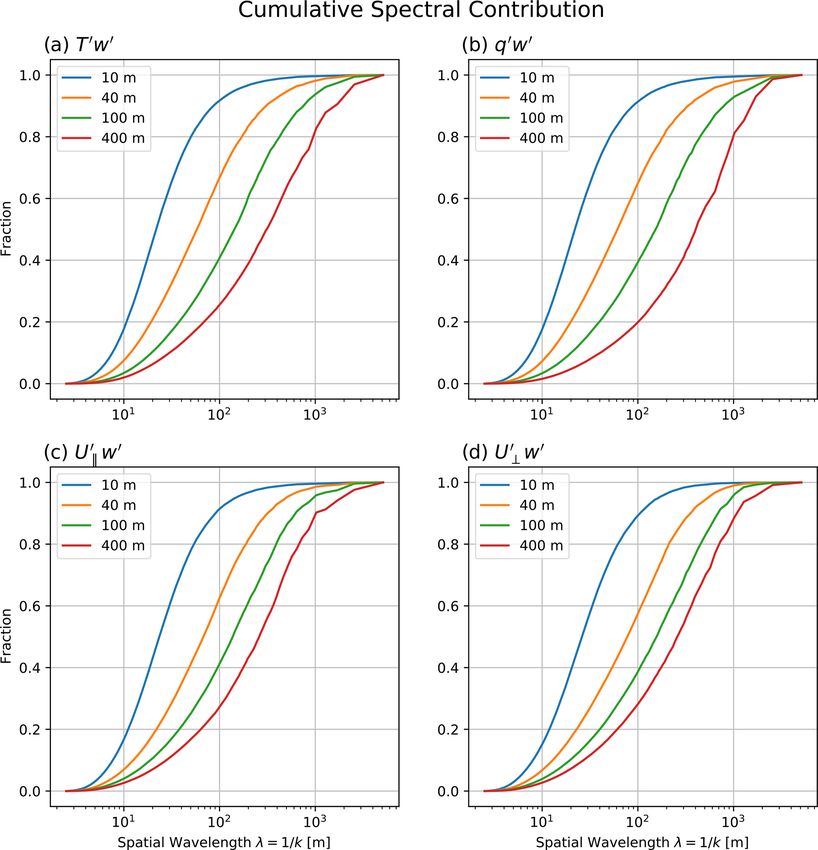
1962                                                                         G. W. Petty: Simulated aircraft flux measurements

                                                                        Throughout this paper, results are highlighted at four rep-
                                                                     resentative heights: 10, 40, 100, and 400 m. For the environ-
                                                                     ment simulated, these correspond to approximately 0.01zi ,
                                                                     0.05zi , 0.12zi , and 0.48zi , respectively. While subjectively
                                                                     chosen, these heights have some correspondence to real-
                                                                     world aircraft observations, including Cook and Renfrew
                                                                     (2015), who observed marine fluxes around the British Isles
                                                                     at an altitude of ∼ 40 m, and the recent Chequamegon Het-
                                                                     erogeneous Ecosystem Energy-balance Study Enabled by a
                                                                     High-density Extensive Array of Detectors 2019 campaign
                                                                     (CHEESEHEAD19), in which the University of Wyoming
                                                                     King Air flew legs at 100 and 400 m (Butterworth et al.,
                                                                     2021). The lowest height of 10 m was included because of
                                                                     interest by the author in potential flux measurements using
                                                                     the University of Wisconsin ultralight research airplane.

                                                                     2.3.1   Spectra

                                                                     Power spectra were computed for vertical velocity w, tem-
                                                                     perature T , specific humidity q, and horizontal wind speed U
                                                                     for each of above levels. This was done by first taking the 2-D
                                                                     Fourier power spectrum of the entire horizontal slice through
Figure 1. Domain-averaged profiles of (a) potential temperature      the domain and then averaging radially to obtain a direction-
θ and (b) specific humidity q at the end of the LES run. Dashed      independent 1-D average power spectrum. For clarity, results
lines indicate the heights of the minimum and maximum altitudes      are shown for only two heights (40 and 400 m) in Fig. 2.
at which non-zero cloud water occurred at any point in the domain.      Figure 2a shows that, at 400 m height (0.48zi ), the LES
                                                                     produces a vertical velocity spectrum approximately obey-
                                                                     ing a Kolmogorov power law for the vertical velocity field
   Consistent with the observed environment on the flight            over more than two decades, from wavelengths greater than
date, the LES was initialized with a boundary layer depth            1 km down to ∼ 8 m or about 3 times the Nyquist wavelength
zi = 840 m delineated by a sharp 8.5 K temperature inver-            of 2.5 m. At this height, peak energy in the spectrum is near
sion. Below zi , the initial potential temperature θ was 289 K       1 km wavelength. At the much lower height of 40 m (0.05zi ),
and the specific humidity q was 9 g kg−1 . These values did          peak energy is found near 150 m, and there is substantially
not change significantly during the simulated evolution of the       less energy at longer wavelengths. In both cases, the peak
boundary layer (Fig. 1). A prescribed sea surface tempera-           energy in w is thus found near ∼ 4 times the physical dis-
ture of 292.5 K was used, leading to domain-averaged sensi-          tance z from the lower boundary, consistent with dominant
ble and latent heat fluxes of 15 and 115 W m−2 , respectively.       contributions from eddies of size z centered at height z.
The wind was initialized as geostrophic; at the conclusion              The spectra for temperature (Fig. 2b) and specific humid-
of the simulation, the mean horizontal wind components (u            ity (Fig. 2c) reveal considerably more energy at the longest
and v) below zi were nearly uniform at 6.7 and −5.0 m s−1 ,          wavelengths, even at 40 m height, while also rolling off ear-
respectively, corresponding to a wind direction of 307◦ (ap-         lier than w at the short wavelength end. The spectrum for
proximately northwesterly) and speed of 8.4 m s−1 .                  temperature is also somewhat flatter than for either w or q.
   The cloud base and top, defined here as the lowest and            The spectrum for horizontal wind speed U (Fig. 2d) is no-
highest levels at which non-zero cloud liquid water occurred         table in having no significant dependence on height, presum-
at any point in the horizontal domain, were found at 500 and         ably because proximity to the lower boundary imposes no
885 m, respectively. This paper is concerned exclusively with        special constraint on horizontal flow in this low-friction, neu-
the subcloud boundary layer at and below 400 m or 0.48zi .           trally stratified environment.
                                                                        Overall, the spectra of scalar variables seem reasonable
2.3    Turbulent structure and domain-averaged fluxes                and give no clear cause to doubt the overall realism of
                                                                     the LES for wavelengths spanning the range from ∼ 10 to
Many details concerning the model run and the overall tur-           ∼ 1 km. Nevertheless, the constraint on the long-wavelength
bulent structure of the simulated boundary layer are given by        end due to the approximately 5 km domain size cannot be
Matheou (2018). Here, we focus on those grid-resolvable tur-         overlooked. While it is easy to discount the importance of
bulent properties most directly relevant to an understanding         the very short wavelengths that are artificially dissipated in
of the simulated flux measurements.                                  the numerical model, it is more difficult to assess the influ-

Atmos. Meas. Tech., 14, 1959–1976, 2021                                                https://doi.org/10.5194/amt-14-1959-2021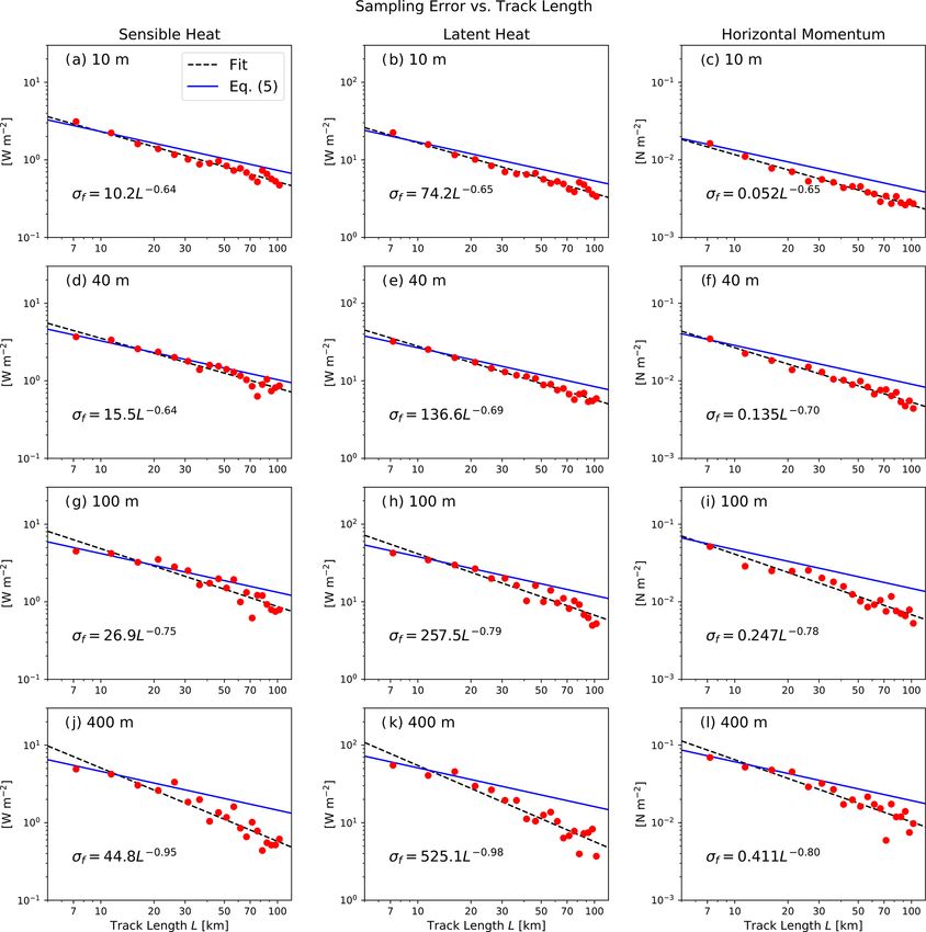
G. W. Petty: Simulated aircraft flux measurements                                                                                   1963

Figure 2. Radially averaged power spectra for selected scalar variables at two representative heights (40 m = 0.05zi and 400 m = 0.48zi ):
(a) vertical velocity, (b) temperature, (c) specific humidity, and (d) horizontal wind speed. For reference, dashed black lines depict the
power-law exponent of −2/3 expected for a Kolmogorov spectrum in the inertial subrange.

ence of the domain size on turbulent structures of the order           3     Flux calculations
of 1 km and greater. de Roode et al. (2004) found that peak
energy for vertical motion and for virtual potential temper-           The local contributions to the turbulent fluxes of sensible heat
ature are found at wavelengths comparable to the boundary              (SH) and latent heat (LH) are
layer depth – which is less than 1 km in the present case –
                                                                       SH0 = ρCp θ 0 w 0                                              (1)
but that humidity and potential temperature can exhibit sig-
nificant variations on larger scales.                                  and

2.3.2   Horizontal cross sections                                      LH0 = ρLq 0 w 0 ,                                              (2)

Horizontal cross sections of temperature T 0 , specific humid-         where ρ is the mean air density at level z, Cp =
ity q 0 , and vertical velocity w0 are presented for these heights     1005 J kg−1 K−1 is the specific heat capacity at constant pres-
in Fig. 3, where the primed quantities indicate instantaneous,         sure, θ 0 is the potential temperature perturbation, and L ≈
local deviations from the domain-averaged value at each                2.5 × 10⁶ J kg−1 is the latent heat of vaporization of water.
height. These show an evolution from predominantly fine-               Note that for the low altitudes and near-standard pressures
scale structure near the surface to consolidated perturbations         p encountered in this simulation, θ 0 = T 0 (100 kPa/p)0.286 ≈
of order 1 km diameter at 400 m. In the w 0 field near the sur-        T 0.
face, there is a visually obvious alignment of structures with            In the above expressions, the common notation LE for la-
the mean wind. This directional anisotropy is far less appar-          tent heat flux is avoided because it implies a product of the la-
ent in q 0 and is completely absent from T 0 at low levels.            tent heat of vaporization L and surface evaporation rate E. At
                                                                       any significant distance above the surface, the actual vertical
                                                                       flux of water vapor measured by an aircraft may or may not
                                                                       equal E. All fluxes described herein should be understood
                                                                       as flight-level fluxes without any assumption about their re-
                                                                       lationship to surface fluxes. To reinforce this distinction, the
                                                                       more generic symbols (SH and LH) have been adopted here.

https://doi.org/10.5194/amt-14-1959-2021                                                   Atmos. Meas. Tech., 14, 1959–1976, 2021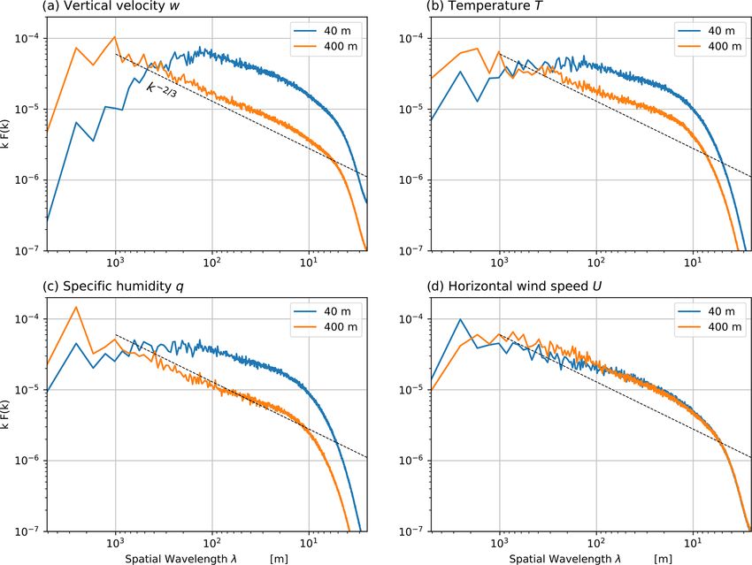
1964                                                                          G. W. Petty: Simulated aircraft flux measurements

Figure 3. Horizontal cross sections of T 0 (left column), q 0 (center column), and w 0 (right column). Rows correspond to 10, 40, 100, and
400 m heights.

   The local u and v components of momentum flux are com-              with the mean wind direction so as to isolate the along-wind
puted as                                                               and crosswind components (Uk , U⊥ ).
                                                                          Figure 4 depicts the ratio of parameterized subgrid-scale
 τu0 , τv0 = ρ · (u0 w0 , v 0 w 0 ).

                                                       (3)             flux to total vertical flux (subgrid-scale plus resolved) as a
Where appropriate in the discussion below, the horizontal              function of height above the surface. At 10 m height, the frac-
wind vector (u, v) is rotated into a coordinate system aligned         tion is less than 5 % for LH and SH and less than 2 % for

Atmos. Meas. Tech., 14, 1959–1976, 2021                                                  https://doi.org/10.5194/amt-14-1959-2021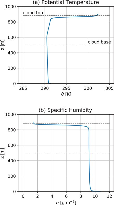
G. W. Petty: Simulated aircraft flux measurements                                                                                             1965

Figure 4. Parameterized subgrid-scale flux as a fraction of total turbulent flux for the LES used in this study. (a) latent heat. (b) sensible heat.
(c) horizontal momentum (figure courtesy of Georgious Matheou, personal communication, 2021).

horizontal momentum flux. Consequently, we can neglect the                  flux error assessments for heights near or below 100 m are
unresolved components of the fluxes for the purposes of this                least likely to be seriously biased by the LES domain size of
study.                                                                      5.12 km, while 400 km may be more susceptible.
   Domain-averaged resolved fluxes and turbulent kinetic en-
ergy (TKE) are depicted in Fig. 5. These fluxes serve as the
nominal “truth” values against which simulated aircraft flux                4     Random error in flux measurements
measurements will be evaluated.
                                                                            4.1    Defining the problem
   As expected, the profile of sensible heat flux (Fig. 5a) is
quite linear except within cloud, where latent heating due to               According to the eddy covariance method, an estimate F̂ψ of
condensation sharply increases the positive correlation be-                 the true turbulent flux Fψ is obtained from a series of closely
tween T and w. It crosses through zero near 445 m (0.53zi ).                spaced measurements of scalar variable ψ and vertical veloc-
The profile of latent heat flux is noticeably less smooth, as               ity w as
are τu and τv (Fig. 5b). Turbulent kinetic energy varies only
weakly below cloud and has a sharp maximum at cloud top,                    F̂ψ ∝ ψ 0 w0 ,                                                      (4)
as expected. (Fig. 5c).                                                     where the proportionality allows for appropriate multiplica-
   Figure 6 presents ogive (cumulative distribution) plots of               tive constants, and the overline indicates an average over time
the spectral contributions to each flux. For all four flux vari-            and/or space, with ψ 0 ≡ ψ−ψ and w 0 ≡ w−w. In the present
ables, there is a pronounced shift from predominantly short-                context, the average is along the length of a flight track and
wavelength contributions at the lowest levels to much lower-                is considered to be effectively instantaneous.
frequency contributions at 400 m. In particular, 90 % of the                   Because of the stochastic nature of turbulence, F̂ψ is in
total sensible heat flux contribution comes from the wave-                  general an imperfect estimate of the true flux Fψ , but one
length ranges [6 m, 146 m], [8 m, 0.51 km], [12 m, 1.0 km],                 that can theoretically improve with a larger sample, subject
and [17 m, 2.6 km] at heights of 10, 40, 100, and 400 m, re-                to assumptions about stationarity. For a single flight track,
spectively, with qualitatively similar ranges for latent heat               the error in the flux estimate is
flux and momentum flux. Overall, these results suggest that
                                                                            δf ≡ F̂ψ − Fψ .                                                     (5)

https://doi.org/10.5194/amt-14-1959-2021                                                         Atmos. Meas. Tech., 14, 1959–1976, 2021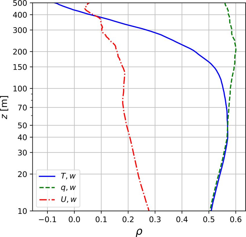
1966                                                                               G. W. Petty: Simulated aircraft flux measurements

Figure 5. Domain-averaged turbulent quantities computed from grid-resolved u0 , v 0 , w 0 , T 0 , and q 0 in the LES simulation.

Figure 6. Ogive plots of the spectral contributions to the total eddy correlation fluxes for (a) sensible heat, (b) latent heat, (c) horizontal
momentum in the along-wind direction, and (d) horizontal momentum in the crosswind direction.

If a large ensemble of identical tracks were flown but suffi-               Eq. 1):
ciently displaced from one another in time and/or space so                                       2 1/2
as to be statistically independent, the mean error would be
                                                                            σψ ≡        F̂ψ − Fψ             .                             (6)
expected to converge to zero, but the uncertainty associated
with any single track could be characterized via the ensem-
ble root-mean-squared error (Lenschow and Stankov, 1986,                      The fundamental problem is to characterize the above ran-
                                                                            dom uncertainty for any particular flight track, given the

Atmos. Meas. Tech., 14, 1959–1976, 2021                                                        https://doi.org/10.5194/amt-14-1959-2021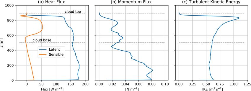
G. W. Petty: Simulated aircraft flux measurements                                                                              1967

length of the track and appropriate assumptions about the             e.g., Sühring and Raasch (2013) or
turbulent environment being measured. An additional com-                      p
plicating factor is that the required true means ψ and w must                  Iw Iψ
themselves be estimated from the finite flight track and will         Iwψ ≤          ;                                          (10)
                                                                              ρw,ψ
therefore also be subject to random errors.
                                                                      e.g., Bange et al. (2002).
4.2     Integral length scales                                           Because all of the above length scales and correlations can
                                                                      be computed directly from the LES fields, it will be possible
4.2.1       Significance
                                                                      to empirically assess the validity of Eqs. (8)–(10).
Central to the problem of estimating random error in aircraft
measurements of turbulent fluxes is the integral length scale,        4.2.2   Determination from LES
also known as the autocorrelation length, of the fields being
                                                                      For each height under consideration, the two-dimensional au-
measured (Lenschow and Stankov, 1986; Lenschow et al.,
                                                                      tocorrelation of the full horizontal model domain was ob-
1994; Sühring and Raasch, 2013):
                                                                      tained for each turbulent field of interest. If was then de-
        Zr0                                                           termined in two orthogonal directions: one aligned with the
If ≡          Af (r) dr,                                       (7)    mean wind (“parallel”) and the other perpendicular (“cross-
        0
                                                                      wind”). Results are shown in Fig. 7. Note that for momen-
                                                                      tum fluxes, the wind vector (u, v) was projected onto the
where Af (r) is the autocorrelation p of generic spatial func-        parallel and crosswind directions to obtain the rotated vector
tion f (x, y) at displacement r = x 2 + y 2 in any specified          (Uk , U⊥ ). Thus, the integral length scale labeled “U⊥ par-
direction, Af (0) ≡ 1, and r0 is the distance to the first zero       allel”, for example, describes that computed for the turbu-
crossing or one-half of the domain diameter (in this case             lent flux of the momentum component perpendicular to mean
2.56 km), whichever is smaller. In the ideal “red noise” case,        wind measured along a track parallel to the mean wind.
Af (r) = exp(−r/If ), and Af (If ) = e−1 . The length scale              A number of general observations can be made concerning
is thus useful for characterizing the minimum track length            the computed values of If :
and/or spatial separation required in order to be able to treat
two sets of measurements as statistically independent.                  – For every variable, If at and below z = 100 m = 0.12zi ,
   Viewed simplistically, for a track length L = N If , the ran-          corresponding roughly to the surface layer, is well ap-
dom error in F̂ψ as an estimate of the true ensemble value                proximated by a straight line on a log–log plot, imply-
should decrease with N −1/2 , consistent with the calcula-                ing an empirical relationship of the form If ≈ Azb . For
tion of standard error for any set of N noisy measurements.               some variables, such as the specific humidity (Fig. 7a)
Richardson et al. (2006) argues persuasively that it is more              and the sensible and latent heat fluxes (Fig. 7f, g), the
natural to focus on the absolute rather than relative random              validity of such a relationship seems to extend consid-
error, as the relative error becomes extremely large or even              erably higher.
undefined in the common case that the flux approaches or
crosses zero, for example, either at sunrise or sunset or near          – For most variables, If is larger for tracks parallel to the
the altitude at which sensible heat flux switches signs. With             mean wind, as expected, than for crosswind tracks, of-
that in mind, Eq. (7) of of Lenschow and Stankov (1986)                   ten considerably larger. Two interesting exceptions are
is rearranged to give the following absolute random uncer-                found in If for temperature above 40 m (Fig. 7b) and
tainty:                                                                   for Uk above 100 m, where the crosswind value of If is
                                                                          up to 50 % greater than for the parallel direction.
                    I 1/2
             −2         wψ
σψ = 2 ρw,ψ      +1              Fψ ,                        (8)
                        L                                               – For many variables (q, U⊥ , w, SH, and LH), the differ-
                                                                          ence between the parallel and crosswind values of If
where ρw,ψ is the zero-lag Pearson correlation coefficient of
                                                                          is largest near the surface and decreases to near zero at
w 0 with ψ 0 , and Iwψ is the integral scale length of w0 ψ 0 .
                                                                          higher altitudes. For temperature, however, the reverse
   Lenschow et al. (1994) and Mann and Lenschow (1994)
                                                                          is true (Fig. 7b).
refer to the difficulty of obtaining estimates of Iwψ and pro-
pose theoretically derived substitutions based on the more
commonly available Iw and Iψ . The problem of convergence               – The three turbulent wind components behave quite dif-
of integral lengths under some circumstances is further dis-              ferently, with If for Uk and U⊥ exhibiting a rela-
cussed by Durand et al. (2000). Subsequent authors, citing                tively weak and non-linear dependence on height, while
Mann and Lenschow (1994), variously utilize                               for the vertical wind component w, the dependence is
        p                                                                 strong. Indeed for the crosswind case, If for w is al-
Iwψ ≤ Iw Iψ ;                                                   (9)       most perfectly proportional to z.

https://doi.org/10.5194/amt-14-1959-2021                                                 Atmos. Meas. Tech., 14, 1959–1976, 2021
1968 G. W. Petty: Simulated aircraft flux measurements
Figure 7. Integral length scales If for the indicated quantities, measured along (“parallel”) and perpendicular to (“crosswind”) the mean
wind direction.
– Of all the variables considered, only the turbulent ki- length scales and −2/3 for the along-wind length scales. It is
netic energy exhibits an integral length scale that is vir- beyond the scope of this paper to investigate the reasons for
tually constant with height throughout the full depth of the discrepancy.
the model domain (Fig. 7i). Apparent in the above results is that Eqs. (9) and (10) gen-
The calculated If results below 100 m were used to ob- erally yield large overestimates of Iwψ for any scalar vari-
tain coefficients A and b for the aforementioned power-law able ψ. For example, at 100 m height and measured p in the
fit. These coefficients are provided in Table 2. Alternatively, crosswind direction, Iq = 220 m and Iw = 73 m. Iq Iw is
If = A? z?b , where z? ≡ z/zi , A? = Azib and zi = 840 m. It is then 127 m, a factor of 2.5 larger than the directly computed
not known to what degree the results found here are transfer- Iwq = 51 m. In general, the minimum overestimate at or be-
able to other environments. low 400 m was found to be about a factor of 2 or greater, with
It is noteworthy that the exponents b found here for fluxes ratios in excess of 3–5 typical at lower heights. The differ-
of sensible heat, latent heat, and horizontal momentum are ence increases further if one uses the correlation coefficient
quite different than the exponent of −1/3 or −1/2 obtained ρw,ψ < 1 in the denominator per Eq. (10). Specific combina-
theoretically by Lenschow and Stankov (1986) for all of tions of variables and heights can be easily examined using
these (their Eq. 11), being closer to −1 for the crosswind the relationships in Table 2.
Atmos. Meas. Tech., 14, 1959–1976, 2021 https://doi.org/10.5194/amt-14-1959-2021G. W. Petty: Simulated aircraft flux measurements 1969
Table 2. Coefficients for the integral length scale If ≈ Azb , valid
up to at least 100 m altitude in this simulation, depending on the
variable (see Fig. 7), where both IL and z are in meters. Also given
is the approximation If ≈ A for selected variables.
A b A
q Crosswind: 20.6 0.51
Parallel: 35.2 0.41
T Crosswind: 20.5 0.56
Parallel: 33.1 0.36
Uk Crosswind: 309 −0.06 278
Parallel: 146 0.09 206
U⊥ Crosswind: 161 0.11 233
Parallel: 387 −0.03 371
w Crosswind: 0.63 1.03 Figure 8. Subcloud profiles of correlations between vertical veloc-
Parallel: 2.95 0.82 ity w and temperature T , specific humidity q, and horizontal wind
speed U .
SH Crosswind: 0.53 0.97
Parallel: 3.01 0.64
LH Crosswind: 0.50 1.00
7.2 km. A continuation of the track would simply resample
Parallel: 2.85 0.69
the same grid points. For φ2 = 63.4◦ , the track makes two
τk Crosswind: 0.91 0.81 widely separated passes through the domain before return-
Parallel: 2.88 0.70 ing to its starting point, and the non-repeating track length
τ⊥ Crosswind: 0.86 0.85 is 11.4 km. The maximum value of n used was 20, for a
Parallel: 2.34 0.79 102.5 km continuous, non-overlapping path.
For any given n, starting points for different tracks of the
TKE Crosswind: 77.3 0.06 96
same length are uniformly distributed along the boundary
Parallel: 95.4 0.05 115
of the domain, maintaining prescribed minimum separation
(measured perpendicular to the paths) intended to ensure a
reasonable degree of statistical independence. These mini-
Also required in the evaluation of random flux errors from mum separations were chosen to be greater than If for all
Eq. (8) is the correlation ρw,ψ between the vertical veloc- relevant variables at the level in question; 20, 50, 100, and
ity w0 and the scalar variable ψ 0 of interest. Computed pro- 150 m were assumed for heights of 10, 40, 100, and 400 m,
files of ρqw,ψ are given in Fig. 8. For horizontal momentum, respectively.
ρw,U = 2 + ρ2 .
ρw,u w,v
The effect of the minimum separation requirement is to
achieve a roughly constant overall sampling density for the
ensemble of tracks of a given length. Thus, Nn is small for
5 Simulated aircraft measurements long tracks and larger for short tracks. By taking mirror im-
ages and 90◦ rotations of the tracks defined in this way, the
5.1 Track definitions total number of distinct tracks available is actually 4Nn , ex-
cept for n = 1, in which case it is 2Nn due to duplication
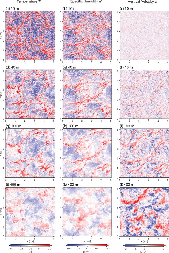
As previously noted, the central purpose of this paper is to when rotating and flipping the 45◦ track patterns. Figure 9
investigate the empirical relationship between sampling er- depicts an example track for n = 3 (top) and the full corre-
ror in turbulent flux measurements and the length of a con- sponding set of 32 distinct tracks (bottom) for a relatively
tinuous, ideal aircraft track through the virtual atmosphere wide minimum separation of 200 m used for visual clarity;
represented by the LES domain. The algorithm for defining the number of distinct tracks is significantly greater in the
these tracks is described below. actual analysis.
First, each track is required to be perfectly periodic, albeit Note that the algorithm described above is more elabo-
with a period L substantially longer than the dimensions of rate than the fixed-angle track definitions utilized by Schröter
the domain. Specifically, track angles relative the x axis are et al. (2000) and Sühring et al. (2019). To reiterate, each track
defined by φn = arctan(n), where n is a positive integer. For of length Li is required to be periodic with period Li , and in-
φ1 = 45◦ , the track makes a single pass through the domain dividual realizations of a given track length are distributed
before returning to its starting point, and the track length is so as to both maximize and equalize their separation, subject
https://doi.org/10.5194/amt-14-1959-2021 Atmos. Meas. Tech., 14, 1959–1976, 20211970 G. W. Petty: Simulated aircraft flux measurements
gardless of the starting point along the track, as long as the
total distance followed by the virtual aircraft is Li .
An unavoidable shortcoming of the method used here is
that track orientations relative to the mean wind cannot be
specified separately, as the absolute orientations are uniquely
determined by the chosen number of passes n though the
domain and thus by the track length. As n increases, the
trend is toward tracks that are oriented mostly north–south
or east–west, whereas the mean wind in this simulation is
from the northwest. Only for n = 1 are the track directions
nearly aligned with or perpendicular to the wind direction.
5.2 Virtual flux observations
The “truth” value for each comparison is the domain-
averaged flux value computed at each level (Fig. 5). These
values utilized the deviations (primed quantities) from the
true ensemble mean values for the entire domain. As mea-
sured against the true values, aircraft measurements are sub-
ject to two statistical sources of error: (1) error in the determi-
nation of the mean values relative to which primed quantities
will be calculated, and (2) insufficient sampling of the fluc-
tuating primed quantities themselves. Our virtual measure-
ments simulate both effects by utilizing the track-determined
mean values rather than the domain-averaged values. Both
sources of error decrease asymptotically to zero in the limit
of an infinitely long flight track, and the flux estimate will
converge on the true ensemble value.
In the finite 5.12 km × 5.12 km horizontal domain of our
LES, there is the additional issue that a single long flight
track can effectively sample the entire domain, so that the
aircraft measurement can converge almost perfectly on the
“true” value from measurements along a long but finite path.
In principle, then, the results obtained herein for long flight
tracks should be considered lower bounds on the expected
random error. However, because of the minimum separation
maintained between parallel segments of a given tracks, we
believe this potential bias is unimportant for the flight track
lengths considered here. More important may be the inabil-
ity of the finite LES domain to reproduce flux variations with
wavelengths greater than the domain size. As previously dis-
cussed for Fig. 6, this seems likely to be an issue mainly at
heights of ∼ 400 m and above.
Figure 9. Example of flight tracks constructed to pass through the Finally, a notable constraint rooted in the availability of
LES domain an integral number of cycles before exactly repeating. only a single time step from the LES is that the virtual air-
(a) A single three-cycle (16.2 km) track. (b) All possible realiza- craft effectively traverses each path instantaneously. We are
tions of three-cycle tracks such that a minimum parallel spacing of in effect relying on Taylor’s “frozen turbulence” hypothe-
200 m between track legs is maintained. sis and, following Lenschow and Stankov (1986), postulate
that this hypothesis is valid in the present case if If < V Tf ,
where If is the integral length scale, V is the speed of the air-
to the aforementioned minimum separations. This allows us craft, and Tf is the autocorrelation time of the flux field be-
to obtain an optimal set of quasi-independent tracks. Con- ing measured. Unfortunately, it is not possible to determine
straining the tracks to be periodic also means that there is by Tf from the single time step available for this study, but for a
definition no trend or unsampled low frequency contribution real-world V ≈ 85 m s−1 similar to that of the University of
to be concerned about – “measured” fluxes are the same re- Wyoming King Air, one would only require Tf > 1 s to sat-
Atmos. Meas. Tech., 14, 1959–1976, 2021 https://doi.org/10.5194/amt-14-1959-2021G. W. Petty: Simulated aircraft flux measurements 1971
Table 3. Coefficients for the empirical fits depicted as dashed black Table 4. Minimum track length L10 in kilometers required to
lines in Fig. 11, where the flux uncertainty σf = BLc , and L is the achieve 10 % uncertainty in flux estimates based on the expression
track length in kilometers. Resulting units are W m−2 for latent and and coefficients in Table 3.
sensible heat fluxes; N m−2 for horizontal momentum flux.
Height Sensible Latent Horizontal
Height Sensible heat Latent heat Horizontal heat heat momentum
momentum 10 m 9.0 9.1 18.0
B c B c B c 40 m 19.1 19.3 60.5
100 m 33.1 29.7 85.7
10 m 10.2 −0.64 74.2 −0.65 0.052 −0.65 400 m 334.9 34.5 410.9
40 m 15.5 −0.64 136.6 −0.69 0.135 −0.70
100 m 26.9 −0.75 257.5 −0.79 0.247 −0.78
400 m 44.8 −0.95 525.1 −0.98 0.411 −0.80
The blue lines represent Eq. (8), where both If and the cor-
relation coefficients ρw,ψ are computed directly from the 2-D
isfy the above inequality for flux measurements at a height of LES-generated fields at each level and represent averages of
100 m, based on the values of If seen in Fig. 7. For a much the crosswind and parallel values. As previously pointed out,
slower aircraft or UAV with an air speed of 20 m s−1 , the re- most simulated flight tracks are neither parallel nor perpen-
quirement for Tf is proportionally longer, but these have the dicular to the mean flow, and the set of available orientations
option of flying at lower altitudes where If is smaller. varies with track length. For both reasons, no single repre-
sentation of Eq. (8) as a curve in Fig. 11 can capture the vari-
ability of If and ρw,ψ . However, especially for longer path
6 Results lengths, most paths cross the mean wind at an oblique angle;
thus, the use of the average (direction-independent) If and
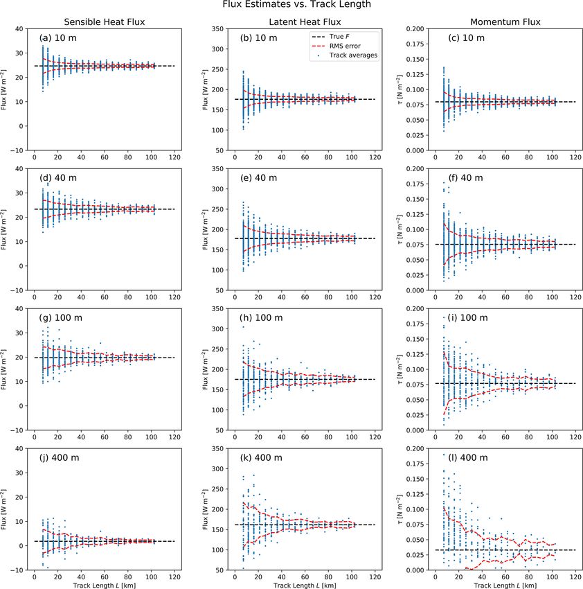
Raw sample results are presented in Fig. 10, with each blue ρw,ψ seems reasonable for this qualitative comparison.
dot representing the estimated flux from a single flight track Finally, from the fits in Table 3, the minimum track lengths
of the indicated length. The true domain-averaged values are L10 required for 10 % relative accuracy are determined.
indicated as dashed black lines, and the root-mean-square These are presented in Table 4.
(rms) deviation from the true value is depicted as a dashed Noteworthy findings include the following:
red line. For all flux variables, there is the expected decay in
sampling error as the track length becomes longer. – Equation (8) due to Lenschow and Stankov (1986) and
Noteworthy features include the following: using the independently computed parameter values is
remarkably accurate at predicting the random error for
– Overall scatter is largest at the highest altitudes, consis- shorter track lengths.
tent with the longer integral length scales If and with
the observation by previous authors that error tends to – Empirical fits generally show a steeper decrease with
increase with height (e.g., Grossman, 1992). track length than the L−1/2 relationship predicted by
Eq. (8), with exponents ranging from −0.64 to −0.70
– For sensible heat flux at 400 m (Fig. 10j), the magni- at 10 and 40 m, to nearly −1 for sensible and latent
tude of the scatter is often far in excess of the very heat fluxes measured at a height 400 m. It is not clear
low (1.8 W m−2 ) mean flux itself, so that shorter track whether the more rapid decay in error is primarily re-
lengths cannot reliably determine even the sign of the lated to the finite domain size – with this issue being
mean flux. most likely problematic at 400 m – or to other depar-
– Relative to the mean values, scatter is particularly large tures from the idealized statistical model of turbulence
for momentum assumed by Lenschow et al. (1994).
p flux. Because this quantity is positive
definite (τ = τu2 + τv2 ), the distribution of errors at
400 m is strongly skewed and positively biased. – For flights at and below 100 m, track lengths of approx-
imately 30 km or less are sufficient to achieve 10 % pre-
Figure 11 offers a closer look at the dependence of sam- cision in sensible and latent heat flux estimates in this
pling error on path length and allows the results obtained to particular environment. Required track lengths for mo-
be compared with the random error predicted by Eq. (8). The mentum flux τ are considerably longer; nearly 90 km at
red dots correspond to the empirical rms error values previ- 100 m height.
ously represented in Fig. 10 as dashed red curves. The dashed
black lines represent fits to those values. The accompanying – At a height of 400 m, no reasonable track length is long
power-law expressions for each fit appears in black as well enough to adequately measure the low sensible heat and
as being summarized in Table 3. momentum fluxes encountered there.
https://doi.org/10.5194/amt-14-1959-2021 Atmos. Meas. Tech., 14, 1959–1976, 20211972 G. W. Petty: Simulated aircraft flux measurements
Figure 10. Flux estimates versus track lengths for sensible heat (left column), latent heat (center column), and horizontal momentum (right
column). Dashed red curves depict the root-mean-squared deviation of estimates from the true domain-averaged flux (horizontal dashed line).
6.1 Uncertainties in flux error determinations on Eq. (8), an error bias factor was defined as
1/2
−2
The previous comparison with Eq. (8) assumed that the rele- ρest + 1 If,est
8 ≡ , (11)
vant integral lengths and correlations were the “true” values. −2
ρtrue + 1 If,true
In practice, it may be necessary when estimating sampling er-
rors to determine these parameters empirically from the flight
tracks themselves. These are thus subject to sampling errors where the “est” subscripts refer to the track-estimated quan-
of their own that in turn imply greater uncertainty in the esti- tities and “true” refers to the domain-averaged quantities.
mation of σ . Thus, the apparent sampling error is given as
To examine this problem, integral lengths If and correla-
tions ρ were estimated directly from the flight tracks. Based σ̂ = 8σ, (12)
Atmos. Meas. Tech., 14, 1959–1976, 2021 https://doi.org/10.5194/amt-14-1959-2021G. W. Petty: Simulated aircraft flux measurements 1973 Figure 11. Relationship between ensemble rms error and track length for sensible heat flux (left column), latent heat flux (center column), and momentum flux (right column). Red dots depict rms deviation of estimates from the true domain-averaged flux, corresponding to the red curves in Fig. 10. An empirical power-law fit is depicted by the dashed black line, with the coefficients of the fit indicated in the expression for σf . The solid blue lines represent Eq. (8) using the parameter values given in Table 3. where σ is the “correct” flux error based on perfect knowl- titudes, the directional dependence of If disappears, as seen edge of the integral length scale and correlation. Results are in Fig. 7g, and so does the apparent bias in the flux error. depicted for LH in Fig. 12. The solid lines depict the aver- At the lowest altitude of 10 m (Fig. 12a), the scatter about age bias factor as a function of track length; the dashed lines the mean bias quickly becomes small with increasing track depict the standard deviation of the bias about this average. length. Surprisingly, this is not the case at 100 or 400 m. Interestingly, at the lowest levels, there is an average low Rather, the relative uncertainty in the flux error is nearly con- bias of between 10 % and 20 %, and this bias persists for the stant with path length. Why this is the case requires further longest track lengths. This is likely an artifact of the method investigation. used, as the track determinations of integral length and corre- Notwithstanding the non-negligible role of sampling un- lation reflect the actual orientation of the track relative to the certainties in If and ρ in estimating the flux uncertainties wind, whereas the generic “true” values do not. At higher al- from Eq. (8), it is perhaps reassuring that the resulting vari- https://doi.org/10.5194/amt-14-1959-2021 Atmos. Meas. Tech., 14, 1959–1976, 2021
1974                                                                      G. W. Petty: Simulated aircraft flux measurements

                                                                   orientations should be practically indistinguishable from true
                                                                   parallel and crosswind flights.
                                                                      Empirical flux errors were determined separately for these
                                                                   two cases, and the results are given in Table 5. With the ex-
                                                                   ception of sensible heat at 400 m, where sampling error is
                                                                   in any case unusably large relative to the true flux, all flux
                                                                   variables are sampled with significantly greater precision in
                                                                   the crosswind direction. The difference is up to about a fac-
                                                                   tor of 2 for latent heat up to at least 100 m and for all variables
                                                                   at the lowest level.

                                                                   7   Conclusions

                                                                   In this paper, the high-resolution large eddy simulation of the
                                                                   marine boundary layer by Matheou (2018) was utilized to
                                                                   determine random flux sampling errors by a virtual aircraft
Figure 12. Distributions of empirically determined bias factors    flying tracks of various lengths at heights of 10, 40, 100, and
from Eq. (11) as functions of track length.                        400 m. We eliminated the need for detrending by construct-
                                                                   ing these tracks to be periodic with periods of the specified
                                                                   lengths.
ations are typically no more than about 10 %, though larger           The empirical results were compared with the theoretically
errors are manifestly possible.                                    derived expression of Lenschow and Stankov (1986). In sup-
   Similar results were found at lower levels for sensible heat    port of these comparisons, we computed the required integral
and momentum flux (not shown). At 400 m, the scatter in            length scales If and found that these are well described by
the bias term for these variables is quite large, reflecting the   expressions of the form If = Azb for z ≤ 100 m, with coef-
small cross correlations found near this level (see Fig. 8).       ficients A and b given in Table 2. The empirical exponents
When ρ is small, even modest sampling errors in the deter-         b are generally between about 2/3 and 1 for fluxes of sensi-
mination of ρ can produce large fluctuations in 8. In short,       ble heat, latent heat, and momentum, in contrast to Lenschow
when sampling error is poor relative to the actual magnitude       and Stankov (1986), who found exponents of 1/3 to 1/2. The
of the flux, even the ability to accurately characterize that      reason for this apparent discrepancy is unknown. The com-
sampling error is impaired.                                        monly cited approximation for the integral length scale for
                                                                   fluxes given by Eq. (9) or (10) was also evaluated and found
                                                                   to consistently overestimate the true value by at least a factor
6.2    The effect of track orientation                             of 2–5.
                                                                      Using directly computed parameter values, Eq. (8) was
As previously noted, the algorithm for track definition, which     shown to be remarkably accurate at predicting random errors
in turn is based on the requirement for periodic tracks, does      for track lengths of approximately 10 km. However, it pre-
not permit the choice of track orientation relative to the wind    dicts a decay in error proportional to L−1/2 , whereas our em-
direction. For this reason, it is not generally possible to use    pirical results show substantially more rapid decay in many
the methods described herein to empirically determine sam-         cases. It is uncertain to what degree the difference is due to
pling error as a function of track length for tracks nearly par-   the finite domain size of the LES, to departures from the
allel or perpendicular to the wind direction.                      idealized statistical assumptions of Lenschow and Stankov
   Having verified that Eq. (8) does appear to give reason-        (1986), or perhaps to a combination of both. It seems less
able results overall for the sampling error (though possibly       likely that the first of these issues would affect the results
overestimating that error for longer track lengths), it follows    for measurements at lower heights, as there is then very little
that the ratio If /L largely determines the sampling error, all    contribution to total fluxes by wavelengths greater than 1 km,
other factors being equal. From the directional dependence         according to Fig. 6.
of If alone, one may infer that flying crosswind should nor-          In general, track lengths of ∼ 30 km or less are sufficient
mally yield smaller errors for a given track length than flying    for measuring sensible and latent heat fluxes in this simu-
parallel to the wind.                                              lated environment to better than 10 % precision, provided
   This assumption may be directly tested in one particu-          that flights are conducted at or below 100 m. Substantially
lar case. For the 7.2 km tracks, corresponding to N = 1, the       longer flight tracks (∼ 85 km) are required for momentum
tracks have an orientation of ±45◦ and thus cross the mean         flux, a result traceable to the low correlation ρU,w (and thus
wind direction of 307◦ at either 8 or 82◦ . Results for these      low corresponding fluxes) between the horizontal and verti-

Atmos. Meas. Tech., 14, 1959–1976, 2021                                              https://doi.org/10.5194/amt-14-1959-2021
G. W. Petty: Simulated aircraft flux measurements 1975
Table 5. For 7.2 km crosswind and parallel tracks, the mean error (bias), and standard deviation σ in simulated flux measurements.
Height Sensible heat Latent heat Horizontal momentum
(W m−2 ) (W m−2 ) (N m−2 10−2 )
True Mean error σ True Mean error σ True Mean error σ
10 m Crosswind 24.7 −0.17 2.02 176.0 −1.11 14.79 7.98 0.125 1.04
Parallel −0.49 3.88 −3.64 27.82 0.079 2.05
Ratio 1.92 1.88 1.97
40 m Crosswind 23.3 −0.25 2.84 177.7 −1.85 22.91 7.55 0.437 2.76
Parallel −0.68 4.32 −6.03 38.89 0.898 3.94
Ratio 1.52 2.05 1.43
100 m Crosswind 19.8 −1.00 3.97 175.4 −8.68 36.18 7.69 1.18 3.94
Parallel −0.89 4.77 −9.12 46.29 2.51 5.46
Ratio 1.20 2.13 1.39
400 m Crosswind 1.8 −0.44 5.60 161.8 −6.24 48.63 3.31 4.05 3.90
Parallel −0.04 4.08 −17.52 57.79 6.78 4.32
Ratio 0.73 1.67 1.11
cal wind components even near the surface. At 400 m height, ing (HEC) Program through the NASA Advanced Supercomputing
only latent heat flux could be estimated with adequate preci- (NAS) Division at Ames Research Center and by the University of
sion using a flight leg of 35 km. On the other hand, legs in Connecticut High Performance Computing (HPC) facility. The pa-
excess of 300 km would theoretically be required to estimate per was significantly improved by comments and suggestions by
sensible heat flux or momentum flux with 10 % precision. Ankur Desai and by two anonymous reviewers. Partial support was
provided by the Chequamegon Heterogeneous Ecosystem Energy-
For comparison, Sühring et al. (2019) found that 200 km
balance Study Enabled by a High-density Extensive Array of De-
flights were desirable to ensure 10 % precision in sensible
tectors (CHEESEHEAD) project.
heat flux estimates within the lower half of the boundary
layer. Their results were obtained for a deep, dry convective
environment. The difference in specific findings undoubtedly Financial support. This research has been supported by the Na-
reflects the larger integral length scales expected in that en- tional Science Foundation (grant no. 1822420).
vironment compared to the shallow, weakly forced marine
boundary layer considered herein. It also highlights the diffi-
culty of extrapolating findings from one environment to an- Review statement. This paper was edited by Thomas F. Hanisco
other. and reviewed by two anonymous referees.
Finally, it was empirically confirmed that for a relatively
short, fixed track length of 7.2 km, flux sampling errors are
reduced up to a factor of 2 by flying crosswind rather than
parallel to the wind, especially at lower levels, consistent References
with the typically shorter integral length scales associated
with the crosswind direction. Bange, J., Beyrich, F., and Engelbart, D. A.: Airborne measure-
ments of turbulent fluxes during LITFASS-98: Comparison with
ground measurements and remote sensing in a case study, Theor.
Appl. Climatol., 73, 35–51, 2002.
Code and data availability. Data sets and Jupyter notebook files
Brilouet, P.-E., Durand, P., and Canut, G.: The marine atmospheric
utilized in the analysis may be requested by sending a 1 TB USB
boundary layer under strong wind conditions: Organized turbu-
drive to the corresponding author.
lence structure and flux estimates by airborne measurements, J.
Geophys. Res.-Atmos., 122, 2115–2130, 2017.
Brilouet, P.-E., Durand, P., Canut, G., and Fourrié, N.: Organized
Competing interests. The author declares that there are no compet- turbulence in a cold-air outbreak: Evaluating a large-eddy simu-
ing interests. lation with respect to airborne measurements, Bound.-Lay. Mete-
orol., 175, 57–91, https://doi.org/10.1007/s10546-019-00499-4,
2020.
Acknowledgements. George Matheou kindly provided the LES data Brooks, I. M. and Rogers, D. P.: Aircraft observations of boundary
set without which this study would not have been possible. It was layer rolls off the coast of California, J. Atmos. Sci., 54, 1834–
in turn created with support from the NASA High-End Comput- 1849, 1997.
https://doi.org/10.5194/amt-14-1959-2021 Atmos. Meas. Tech., 14, 1959–1976, 2021You can also read