Scale-Localized Abstract Reasoning
←
→
Page content transcription
If your browser does not render page correctly, please read the page content below
Scale-Localized Abstract Reasoning

                                                                        Yaniv Benny1                 Niv Pekar1                Lior Wolf1,2

                                                                       1
                                                                           The School of Computer Science, Tel Aviv University
                                                                                    2
                                                                                      Facebook AI Research (FAIR)
arXiv:2009.09405v2 [cs.AI] 26 Jul 2021

                                                                  Abstract                                     applying machine learning models to it can sometimes re-
                                                                                                               sult in shallow heuristics that have little to do with actual
                                             We consider the abstract relational reasoning task,               intelligence. Therefore, it is necessary to study the pitfalls
                                         which is commonly used as an intelligence test. Since                 of RPMs and the protocols to eliminate these exploits.
                                         some patterns have spatial rationales, while others are only              In Sec. 2.1, we present an analysis of the most pop-
                                         semantic, we propose a multi-scale architecture that pro-             ular machine learning RPM benchmarks, PGM [15] and
                                         cesses each query in multiple resolutions. We show that in-           RAVEN [26], from the perspective of biases and exploits. It
                                         deed different rules are solved by different resolutions and          is shown that RAVEN is built in a way that enables the se-
                                         a combined multi-scale approach outperforms the existing              lection of the correct answer with a high success rate with-
                                         state of the art in this task on all benchmarks by 5-54%.             out observing the question itself. To mitigate this bias, we
                                         The success of our method is shown to arise from multiple             construct, in Sec. 3, a fair variant of the RAVEN bench-
                                         novelties. First, it searches for relational patterns in multi-       mark. To further mitigate the identified issues, we propose
                                         ple resolutions, which allows it to readily detect visual re-         a new evaluation protocol, in which every choice out of the
                                         lations, such as location, in higher resolution, while allow-         multiple-choice answers is evaluated independently. This
                                         ing the lower resolution module to focus on semantic rela-            new evaluation protocol leads to a marked deterioration in
                                         tions, such as shape type. Second, we optimize the reason-            the performance of the existing methods and calls for the
                                         ing network of each resolution proportionally to its perfor-          development of more accurate ones that also allows for a
                                         mance, hereby we motivate each resolution to specialize on            better understating of abstract pattern recognition. In Sec. 4,
                                         the rules for which it performs better than the others and ig-        we propose a novel neural architecture, which, as shown in
                                         nore cases that are already solved by the other resolutions.          Sec. 5, outperforms the existing methods by a sizable mar-
                                         Third, we propose a new way to pool information along the             gin. The performance gap is also high when applying the
                                         rows and the columns of the illustration-grid of the query.           network to rules that were unseen during training. Further-
                                         Our work also analyses the existing benchmarks, demon-                more, the structure of the new method allows us to separate
                                         strating that the RAVEN dataset selects the negative exam-            the rules into families that are based on the scale in which
                                         ples in a way that is easily exploited. We, therefore, propose        reasoning occurs.
                                         a modified version of the RAVEN dataset, named RAVEN-                     The success of the new method stems mostly from
                                         FAIR. Our code and pretrained models are available at                 two components: (i) a multi-scale representation, which is
                                         https://github.com/yanivbenny/MRNet.                                  shown to lead to a specialization in different aspects of the
                                                                                                               RPM challenge across the levels, and (ii) a new form of in-
                                                                                                               formation pooling along the rows and columns of the chal-
                                         1. Introduction                                                       lenge’s 3 × 3 matrix.
                                                                                                                   To summarize, the contributions of this work are as fol-
                                            Raven’s Progressive Matrices (RPM) is a widely-used                lows: (i) An abstract multi-scale design for relational rea-
                                         intelligence test [13, 3], which does not require prior knowl-        soning. (ii) A novel reasoning network that is applied on
                                         edge in language, reading, or arithmetics. While IQ mea-              each scale to detect relational patterns between the rows and
                                         surements are often criticized [21, 4], RPM is highly corre-          between the columns of the query grid. (iii) An improved
                                         lated with other intelligence-based properties [17] and has           loss function that balances between the single positive ex-
                                         a high statistical reliability [12, 11]. Its wide acceptance          ample and the numerous negative examples. (iv) A multi-
                                         by the psychological community led to an interest in the AI           head attentive loss function that prioritizes the different res-
                                         community. Unfortunately, as pointed out by [20, 25, 8],              olutions to specialize in solving different rules. (v) A new

                                                                                                           1
balanced version of the existing RAVEN dataset, which we
call RAVEN-FAIR.

2. Related Work and Dataset Analysis
    The first attempt in an RPM-like challenge with neural
networks involved simplified challenges [6]. The Wild Re-
lation Network (WReN) [15], which relies on the Relation
Module [16], was the first to address the full task and in-
troduced the PGM benchmark. WReN considers the possi-
ble choices one-by-one and selects the most likely option.
Two concurrently proposed methods, CoPINet [27] and
LEN [28] have proposed to apply row-wise and column-
wise relation operations. Also, both methods benefit from                          (a)                          (b)
processing all eight possible choices at once, which can             Figure 1. Dataset examples. (a) PGM. (b) RAVEN. The rules are
improve the reasoning capability of the model, but as we             annotated and the correct answer is highlighted.
show in this work, has the potential to exploit biases in
the data that can arise during the creation of the negative
choices. CoPINet applies a contrast module, which sub-               The objective is to choose the missing ninth image of the
tracts a common factor from all choices, thereby highlight-          grid out of the eight presented choices, by identifying one
ing the difference between the options. LEN uses an ad-              or more recurring patterns along the rows and/or columns
ditional “global encoder”, which encodes both the context            of the grid. The correct answer is the one that fits the most
and choice images into a single global vector that is con-           patterns. See Fig. 1 for illustration.
catenated to the row-wise and column-wise representations.              PGM is a large-scale dataset consisting of 1.2M train,
The latest methods, MXGNet [24] and Rel-AIR [18], have               20K validation, and 200K test questions. All images in
proposed different complex architectures to solve this task          the dataset are conceptually similar, each showing various
and also consider all choices at once.                               amounts of lines and shapes of different types, colors, and
    Zhang et al. [28] also introduced a teacher-student train-       sizes. Each question has between 1-4 rules along the rows
ing method. It selects samples in a specialized category-            or columns. Each applies to either the lines or the shapes in
and difficulty-based training trajectory and improves per-           the image. Fig. 1(a) shows an example of the dataset.
formance. In a different line of work, variational autoen-              RAVEN is a smaller dataset, consisting of 42K train,
coders [10] were shown to disentangle the representations            14K validation, and 14K test questions divided into 7 dis-
and improve generalization on held-out rules [19]. Our               tinct categories. Each question has between 4-8 rules along
method shows excellent performance and better generaliza-            the rows only. Fig. 1(b) shows an example of the dataset.
tion to held-out rules without relying on either techniques.
    When merging different outputs of intermediate paths,            Evaluation protocols Both datasets are constructed as a
such as in residual [5] or shortcut [1, 14, 23] connections,         closed-ended test. It can be performed as either a multiple-
most methods concatenate or sum the vectors into one. This           choice test (MC) with eight choices, where the model can
type of pooling is used by the existing neural network RPM           compare the choices, or as a single choice test (SC), where
methods when pooling information across the grid of the              the model scores each choice independently and the choice
challenge. In Siamese Networks [2], one compares the out-            with the highest score is taken. While this distinction was
puts of two replicas of the same network, by applying a dis-         not made before, the previous works are divided in their ap-
tance measure to their outputs. Since the pooling of the             proach. WReN follows the SC protocol and CoPINet, LEN,
rows and the columns is more akin to the task in siamese             MXGNet, and Rel-AIR, all followed the MC protocol.
networks, our method generalizes this to perform a triple                In the SC scenario, instead of presenting the agent with
pair-wise pooling of the three rows and the three columns.           all the choices at once, it is presented with a single choice
                                                                     and has to predict if it is the right answer or not. The con-
2.1. Datasets
                                                                     straint of solving each image separately increases the diffi-
   The increased interest in the abstract reasoning chal-            culty since the model cannot make a decision by comparing
lenges was enabled by the introduction of the PGM [15]               the choices. While this eliminates the inter-choice biases,
and RAVEN [26] datasets. These datasets share the same               the agent may label multiple or zero images as the correct
overall structure. The participant is presented with the first       answer and opens the door to multiple success metrics. In
eight images of a 3x3 grid of images, called the context im-         order to directly compare models trained in the MC and SC
ages, and another eight images, called the choice images.            protocols, we evaluate both types of models in a uniform

                                                                 2
manner: the score for all models is the accuracy for the Algorithm 1: RAVEN-FAIR
multiple-choice test, where for the SC-trained model, we input : C - 8 context components
consider the answer with the highest confidence, regardless a - the correct answer for C
of the number of positive answers. output: A - 8 choice components (a ∈ A)
A← − {a};
Dataset Analysis When constructing the dataset for ei- while length(A) < 8 do
ther the MC or the SC challenge, one needs to be very a0 ←− Choice(A);
careful in how the negative examples are selected. If the − M odif y(a0 );
â ←
negative examples are too obvious, the model can eliminate if Solve(C, â) = False then
them and increase the probability of selecting the correct A←− A ∪ {â};
answer, without having to fully identify the underlying pat- end
tern. Negative examples are therefore constructed based on end
the question. However, when the negative examples are all
conditioned on the correct answer, in the MC scenario, the
agent might be able to retrieve the correct answer by looking
at the choices without considering the context at all. For ex-
ample, one can select the answer that has the most common
properties with the other answers. See the supplementary
for an illustration of such biases in a simple language-based
multiple-choice test.
A context-blind test, which is conducted by training a
model that does not observe the context images, can check
whether the negative answers reveal the correct answer. Ide-
ally, the blind test should return a uniform random accu-
(a) (b)
racy, e.g. 12.5% for eight options. However, since the
Figure 2. Illustration of negative examples’ generation processes.
negative choices should not be completely random so that (a) RAVEN. (b) RAVEN-FAIR.
they will still form a challenge when the context is added,
slightly higher accuracy is acceptable. When introduced,
the PGM dataset achieved a blind test score of 22.4%. In the and iteratively enlarges this set, by generating one negative
RAVEN benchmark, the negative examples are generated example at a time. At each round, one existing choice (ei-
by changing a single attribute from the correct image for ther the correct one or an already generated negative one) is
each example, making it susceptible to a majority-based de- selected and a new choice is created by changing one of its
cision. RAVEN was released without such a context-blind attributes. The result is a connected graph of choices, where
test, which we show in the supplementary that it fails at. the edges represent an attribute change.
Concurrently to our work, Hu et al. [7] have also dis-
As an example, we show the process of generating the
covered the context-blind flaw of RAVEN. They propose an
negative examples for RAVEN in Fig. 2(a). For compari-
adjustment to the dataset generation scheme that eliminates
son, we also show the process of how our proposed algo-
this problem, which they call ‘Impartial-RAVEN’. Instead
rithm generates the negative examples for RAVEN-FAIR
of generating the negative choices by changing a random
in Fig. 2(b). Note that the two figures show the produced
attribute from the correct answer, they propose to sample in
choices for different context questions. In each figure, eight
advance three independent attribute changes and generate
choices for an initial question are shown. The center image,
seven images from all the possible combinations of them.
which is also highlighted, is the correct answer. Each arrow
represents a newly generated negative example based on an
3. RAVEN-FAIR
already existing choice, by changing one arbitrary attribute.
In the supplementary, we analyze both PGM and The dotted lines connect between choices that also differ by
RAVEN under the blind, SC, and MC settings. As we show, one attribute but were not generated with condition to each
due to the biased selection of the negative examples, the other. As can be seen, the RAVEN dataset generates the
RAVEN dataset fails the context-blind test, as it is solved questions in a way that the correct answer is always the one
with 80.17% accuracy by only looking at the choices, mak- with the most shared attributes with the rest of the examples.
ing it unsuitable for the MC protocol. The negative option with the most neighbors in this example
We, therefore, propose a modified dataset we term is the top-left one, which only has three neighbors, while the
RAVEN-FAIR, generated by Algorithm. 1. This algorithm correct answer always has eight. Even without highlighting
starts with a set of choices that contains the correct answer the correct answer, it would be easy to point out which one
3it is, by selecting the one with the most neighbors, without Relation Module Based on the encoding of the images,
looking at the question. we apply a relational module (RM) to detect patterns on
In contrast, our fair algorithm generates the negative ex- each row and column of the query. There are three such
amples in a more balanced way. Since each newly generated modules (RMh , RMm , RMl ). For each resolution t ∈
negative choice can now be conditioned on both the correct {h, m, l}, the 9 encodings ent for n = 1, 2, .., 8, a are posi-
image or an already existing negative one, the correct choice tioned on a 3x3 grid, according to the underlying image I n ,
cannot be tracked back by looking at the graph alone. In see Fig. 3(c). The rows and columns are combined by con-
this example, the correct answer only has two neighbors, catenating three encodings on the channel dimension. The
and both the right and top-right negative images have three rows consist of the three triplets (e1t , e2t , e3t ), (e4t , e5t , e6t ),
neighbors. Because the algorithm is random, the number of (e7t , e8t , eat ). Similarly, the columns consist of the three
neighbors that the correct image has is arbitrary across the triplets (e1t , e4t , e7t ), (e2t , e5t , e8t ), (e3t , e6t , eat ). Each row and
dataset, and is between one and eight. column is passed through the relation network (RN).
In the context-blind test (supplementary), RAVEN-FAIR
returned a 17.24% accuracy, therefore passing the test and rt1 = RNt (e1t , e2t , e3t ), c1t = RNt (e1t , e4t , e7t )
making it suitable for both SC and MC. The PGM dataset rt2 = RNt (e4t , e5t , e6t ), c2t = RNt (e2t , e5t , e8t ) (2)
passed our context-blind test as well, with 18.64% accuracy.
rt3 = RNt (e7t , e8t , eat ), c3t = RNt (e3t , e6t , eat )
4. Method Each RN consists of two residual blocks with two convolu-
Our Multi-scale Relation Network (MRNet), depicted in tion layers inside each one. For the high and middle reso-
Fig. 3(b), consists of five sub-modules: (i) a three-stage en- lutions, the convolution has a kernel of size 3 with ’same’
coder Et , where t ∈ {h, m, l}, which codes the input con- padding, while for the low resolution the kernel size is 1
text and a single choice image into representations in three without padding. The output of each relation block is of the
different resolutions: 20 × 20 (high), 5 × 5 (med) and 1 × 1 same shape as its corresponding encoding et , i.e. RNh :
(low), (ii) three relation modules RMt , one for each resolu- R3∗64,20,20 → R64,20,20 , RNm : R3∗128,5,5 → R128,5,5 ,
tion, which perform row-wise and column-wise operations and RNl : R3∗256,1,1 → R256,1,1 . Note that we apply the
on the encodings to detect relational patterns, (iii) three pat- same relation networks to all rows and columns. This ap-
tern modules P Mt , one for each resolution, which detects if proach allows comparison between the rows and between
similar patterns occur in all rows or columns, (iv) three bot- the columns to detect recurring patterns. In addition, it
tleneck networks Bt , which merge the final features of each maintains the permutation and transpose invariance prop-
resolution, and (v) a predictor module M LP , which esti- erty we assume on the rows and columns.
mates the correctness of a given choice image to the context
in question, based on the bottlenecks’ outputs. The model Pattern Module At this point, at each level t ∈ {h, m, l}
is presented with a question in the form of 16 images: a set the representation of the panel is structured as three row
of context images IC = {I n |n ∈ [1, 8]} and a set of choice features and three column features, which we want to merge
images IA = {Ian |n ∈ [1, 8]}. Since the model operates in into a single representation. The module dedicated to this is
the SC protocol, it evaluates the choices separately. There- the pattern module (PM), which applies some operator F (·)
fore, the notations act as if there is only a single choice im- on the rows and columns. It is depicted in Fig. 3(d).
age I a to answer. To solve all eight choices, the model is To promote order-invariance between the three rows or
repeated eight times with a different choice image Ia ∈ IA . columns, a permutation-invariant operator F (·) is recom-
mended. One can perform sum pooling (SUM3). This kind
Multi-scale encoder The encoder is a three-stage Con- of approach was employed by [15, 27, 28]. Due to the lin-
volutional Neural Network that encodes all images (con- earity of the sum pooling, a ReLU is employed.
text or choice) into multi-resolution representations (high,
middle, low). Every image I n ∈ [−1, 1]1,80,80 , for n ∈ SUM3(x1 , x2 , x3 ) := ReLU(x1 + x2 + x3 ) (3)
{1, 2, ..., 8, a}, is passed sequentially through the three
stages of the encoder, i.e., the middle resolution encoding is The reduction is then applied on the rows and columns.
obtained by applying further processing to the output of the
high resolution encoder and similarly the low resolution en- rt = SUM3(rt1 , rt2 , rt3 ), ct = SUM3(c1t , c2t , c3t ) (4)
coding is obtained by further processing the middle resolu-
tion one. Specifically, the encoding process results in three The SUM3 operator has a drawback in that it does not de-
tensors. enh ∈ R64,20,20 , enm ∈ R128,5,5 and enl ∈ R256,1,1 . tect similarity between the rows and between the columns.
Instead, we propose a novel method that is inspired by
enh = Eh (I n ), enm = Em (enh ), enl = El (enm ) . (1) Siamese Networks, which compares multiple rows and
4Figure 3. MRNet. (a) Depiction of the input query. (b) High-level diagram of the architecture. (c) The relation module (RMt ). (d) The
pattern module (P Mt ).
columns. This vector operator DIST3 is defined per vec- purpose, each representation is downsampled by a bottle-
tor index i and is applied to the rows and columns: neck network (Bt ) that encodes the panel representation pt
into feature vectors with 128 features.
DIST3i (x1 , x2 , x3 ) :=(x1,i − x2,i )2
vt = Bt (pt ) (9)
+(x2,i − x3,i )2 (5)
+(x3,i − x1,i )2 The three final features are then concatenated into a single
vector with 384 features (3x128).
rt = DIST3(rt1 , rt2 , rt3 ), ct = DIST3(c1t , c2t , c3t ) (6)
v = Concat(vh , vm , vl ) (10)
DIST3 does not contain an activation function, since the
method is already non-linear. Its advantage is also visible The predictor The resulting merged feature vector from
in its backward path. The gradient of each operator with the bottleneck module is used to predict the correctness of
respect to element i of x1 is: a choice I a ∈ IA to the context IC . A Multi-Layer Per-
ceptron (MLP) predicts the score of the choice images. A
∂SUM3i (x1 , x2 , x3 ) sigmoid translates this score to the probability of the choice
=1
∂x1,i I a to be a correct answer:
(7)
∂DIST3i (x1 , x2 , x3 )
= 2 · (2 · x1,i − x2,i − x3,i ) p(y = 1|I a , IC ) = Sigmoid(M LP (v)) (11)
∂x1,i
For each choice image, the loss is the Binary Cross Entropy
The gradient of SUM3 does not depend on the values of loss. Because each grid has seven negative choices and only
x2 and x3 , while the gradient of DIST3 does. Therefore, one correct answer, we weight the loss of each choice re-
DIST3 has the potential to encourage increased coordina- spectively, meaning that the correct answer has a weight of
tion between the paths. 7 and each negative answer has a weight of 1.
Finally, the row- and column-features are summed into a
merged representation of the entire panel:
Multi-head attentive predictor Optimizing the three
heads with the main loss works relatively well, but we have
pt = rt + ct (8)
found that adding an objective that optimizes each head sep-
arately improves the final results and reduces the overall
Bottleneck module The three relation modules and their training time. To do so, three additional predictors were cre-
pattern detectors return a latent representation of the panel ated, one for each bottleneck output vh , vm , vl . The archi-
in three resolutions (ph , pm , pl ). This module collects the tecture of the heads is the same as that of the main head and
three representations into a single representation. For this the loss function is identical. To encourage each resolution
5to specialize in the rules that the other resolutions are having Test Accuracy (%)
difficulty with, we propose an attentive weight distribution
on the loss functions of the three heads. Consider the pre- Model PGM RAVEN
diction of each head pt (y = y ∗ |I a , IC ) for t ∈ {h, m, l}, Name Version SC base meta FAIR orig
where y ∗ ∈ {0, 1} represent whether the choice I a is cor- ResNet-SC 3 †
48.9 - † 58.3 † 40.4
SC Baselines
rect or not. The weight applied to each head is:
WReN’18 normal 3 62.6 76.9 † 30.3 † 16.8
∗ a
exp{pt (y = y |I , IC )} V-WReN’18 Normal 3 64.8 - - -
wt = P ∗ a
(12) CoPINet’19 no-contrast 3 †
42.7 † 45.2 † 36.5 † 18.4
τ exp{pτ (y = y |I , IC )} †
LEN’19 global-8 3 65.6 † 79.6 † 50.9 † 29.9
Let Lt be the Binary Cross Entropy loss for head t ∈ MRNet 3 93.4 92.6 86.8 84.0
{h, m, l}. The final multi-head loss is:
X no L3 3 84.4 88.4 84.0 80.1
Ablation
L3 = wt Lt (13) no L3 , no wb 3 75.2 84.9 80.6 78.6
t no L3 , no wb, with SUM3 3 74.3 79.0 77.0 69.6
no wb 3 87.6 88.9 83.4 80.2
Training method We trained with a batch size of 32
with SUM3 3 83.2 85.3 79.5 78.2
queries with an early stopping scheme of 20 epochs, mea-
†
suring the accuracy on the validation set. The reported accu- ResNet-MC 7 41.1 - † 24.5 † 72.5
racy was measured on the test set, for the checkpoint with CoPINet’19 normal 7 56.4 † 51.1 † 50.6 91.4
MC Baselines
the best validation accuracy. See supplementary for a de- LEN’19 normal 7 68.1 82.3 † 51.0 72.9
tailed description of the architecture. We did not tune any LEN’19 teacher-model 7 79.8 85.8 - 78.3
hyper-parameter of the model. Adam [9] was used with T-LEN’19 normal 7 70.3 84.1 7 7
lr=1e-3, β=(0.9,0.999), and weight decay of 1e-6. T-LEN’19 teacher-model 7 79.8 88.9 7 7
MXGNet’20 7 66.7 89.6 - 83.9
5. Experiments Rel-AIR’20 7 85.5 - - 94.1
We experiment on PGM, RAVEN, and RAVEN-FAIR. MRNet with-contrast 7 94.5 92.8 88.4 96.6
Each dataset has a preset train, validation, and test splits of
Ablation
no L3 7 85.7 89.0 85.2 95.5
the data. We used the train set for training and the test set no L3 , no wb 7 76.4 85.4 81.3 94.3
for the evaluation. The validation set was used to pick the no wb 7 87.4 89.8 86.1 95.0
best checkpoint during training for evaluation. PGM has
Table 1. Evaluation on all datasets. † Baseline was run by us, due
additional metadata of the rules logic, which can be used
to missing results.
as additional supervision during training. The use of the
metadata has been shown to improve performance on all
previous works. We refer to this more informative setting as Accuracy (%)
PGM meta. Following previous works, the utilization of the Baselines MRNet
metadata was done by extending the predictor module with
an additional head that predicts the 12 bits of the metadata, Regime WReN V-WReN MXGNet (a) (b)
and training the model with an additional (auxiliary) Cross Neutral 62.6 64.2 66.7 75.2 93.4
Entropy loss. Similar to the previous works, the weight for Interpolation 64.4 - 65.4 67.1 68.1
the auxiliary loss is β = 10. Extrapolation 17.2 - 18.9 19.0 19.2
Baselines We compare our method to the state of HO Pairs 27.2 36.8 33.6 37.8 38.4
the art methods: WReN [15], LEN [28], CoPINet [27], HO Triple Pairs 41.9 43.6 43.3 53.4 55.3
MXGNet [24], and Rel-AIR [18]. We also employed the HO Triples 19.0 24.6 19.9 25.3 25.9
ResNet [5] models described in the supplementary: ResNet- HO line-type 14.4 - 16.7 27.0 30.1
SC and ResNet-MC. The former evaluates each choice sep- HO shape-color 12.5 - 16.6 16.9 16.9
arately and the latter all choices at once. Table 2. Generalization evaluation on the held-out regimes of
As noted in Sec. 2, LEN and CoPINet follow the MC PGM. (a) Without weight balancing and L3 . (b) With them.
protocol. To evaluate these baselines without the possibil-
ity of exploiting the weaknesses of RAVEN, we have cre-
ated additional versions of them for the SC protocol. In the contrasting module (‘no-contrast’), which allows infor-
LEN, the ‘global-CNN’ originally accepted all 16 images, mation to pass between the choices. We also compared to
including the choices. We have changed it to accept only LEN with their proposed teacher-model training schedule,
the context images (‘global-8’). In CoPINet, we removed and to T-LEN, which has dedicated prediction paths for line
6(a) (b) (c)
Figure 4. Ablation on the role of each scale in PGM, using a fully trained MRNet on the SC protocol. (a) Without auxiliary loss (PGM),
no L3 . (b) With auxiliary loss (PGM meta), no L3 . (c) Wihout auxiliary loss (PGM), with L3 . We measured the accuracy for each type,
using only one of the scales and the other ones are masked. The inner radius shows the accuracy of the full model. The three rings show
the accuracy of each resolution. The inner ring is the low resolution, then the middle, and the high resolution is the outer one.
Scales Configurations. Accuracy(%) 3.2%, 37.4% and 4.9% respectively. Except for RAVEN,
our SC protocol model even performed better than both SC
h m l All Center 2×2 3×3 L-R U-D O-IC O-IG
and MC protocols of the baselines, despite the SC protocol
3 7 7 72.0 84.1 47.2 48.3 90.0 91.5 87.6 55.5 having less information. We noticed that our model’s per-
7 3 7 73.3 90.5 56.1 53.4 83.5 83.0 82.5 64.1 formance has reached a point where the auxiliary task of the
7 7 3 58.9 97.7 62.2 62.8 42.3 42.5 56.8 48.1 metadata hurts performance since the added task creates a
3 3 7 77.7 82.8 61.7 59.5 91.7 92.2 89.9 66.3 burden on the optimization of the main task (Vapnik et al.
3 7 3 78.3 91.0 63.2 64.7 88.8 92.2 87.7 60.3 (1998) [22]) and does no longer benefit the model. There-
7 33 76.6 98.3 67.5 65.4 81.6 83.4 81.5 58.3 fore the accuracy on PGM meta is lower than that of PGM,
which is the first time a model shows such behavior.
3 33 80.6 87.7 64.7 64.3 94.2 94.3 90.9 68.0 For ablation, we trained our model with the SUM3 oper-
with L3 86.8 97.0 72.7 69.5 98.7 98.9 97.6 73.3 ator instead of DIST3, without the weight balancing of the
Table 3. Ablation on the role of each scale in RAVEN-FAIR positive choices versus the negative ones (no wb), and with-
out the multi-head attentive loss (L3 ). The results are shown
rules and shape rules and is only applicable to PGM. The in Tab. 1 below those of the full model. For SC, we show an
results can be seen in Tab. 1 separately for each protocol. aggregated ablation on these modifications, i.e., each fol-
lowing instance applies an additional modification. Each
Results Before evaluating our model, two important added modification results in a performance decline com-
things can be noticed by observing at the baselines. First, pared to the previous version. The experiments which re-
the performance of LEN and CoPINet declines in SC, move one component at a time also support that both multi-
where unlike MC, the models cannot compare the choices head attentive loss and the weight balancing both greatly
within the model. This is especially noticeable in RAVEN, improve the training of the main head. It is also evident that
where CoPINet practically solved it in MC and failed it in DIST3 is a superior pooling operator over SUM3. For MC,
SC. On both RAVEN and RAVEN-FAIR, all SC baselines we performed an ablation with either or both the weight bal-
performed worse than the simple ResNet-SC, which does ancing and the L3 removed. The simplified models without
not have any dedicated modules for relational reasoning. these contributions are not competitive.
Second, by comparing each models’ performance between
Aside from test accuracy, model capacity and training
RAVEN and RAVEN-FAIR, we can see that MC mod-
resource consumption is also an important factor. While
els perform significantly lower on RAVEN-FAIR than on
our method outperforms the other baselines, it is not bigger
RAVEN. This confirms that RAVEN-FAIR indeed fixes the
or slower to train. Our method trains in about 40 minutes
biases in the data and is much more suitable as a benchmark
per epoch on PGM on a single 1080TI GPU, which is about
than RAVEN, especially for the MC protocol. These obser-
the same speed as WReN and CoPINet, and about 3x faster
vations align with the dataset analysis presented in the sup-
than LEN. We did not measure the runtime of MXGNet,
plementary, which conclusions were discussed in Sec. 2.1.
Rel-AIR, or LEN with the teacher-model framework, but
One can observe that our model outperforms the base-
we expect them to require substantial resources and time.
lines in both protocols and across all datasets. In SC, our
method outperforms previous baselines by 27.8% in PGM, Generalization An important property of a model that is
13.0% in PGM meta, 35.9% in RAVEN-FAIR, and 54.1% good at abstract reasoning is to be able to generalize over
in RAVEN. In MC, we outperform the baselines by 9.0%, rules that were not seen during training. PGM has specially
7built versions of the dataset for this purpose. Aside from the tion is specialized in shape-number, likely because the 3×3
‘Neutral’ regime, there are seven more regimes, where dif- grid alignment of the shapes in each individual image ICn
ferent rule types were omitted from the train and validation of PGM (not to be confused with the 3×3 question align-
sets, and the test set consists solely of the held-out rules. ment) is close to the 5×5 shaped matrix of the encodings
For more details, please refer to Santoro et al. [15]. em . The analysis of the model trained on PGM meta shows
Tab. 2 shows that our method generalizes better in all specifically where the added auxiliary loss contributes. All
regimes. Most notably are the ’HO line-type’ and ’HO resolutions improved their area of expertise from the set-
Triple Pair’ regimes, where our method has a gap of 10% ting without the metadata and learned to solve additional
from the baselines. We do note, however, that other tasks. Some rules were already solved without the auxiliary
regimes, such as ’HO shape-color’ and ’Extrapolation’, loss, such as ’shape-number’ and ’line-type, but others, such
only made a negligible improvement on the baselines and as ’shape-color’ and ’shape-type’, received a substantial in-
are still only slightly better than random. This reassures crease in accuracy. L3 showed a large improvement on all
that there is still much to be done for future work in this rules and better utilization of the middle resolution, without
regard. In the generalization experiments, training with L3 having to use the metadata. The exact results on each rule
only showed minor improvement. We, therefore, conclude can be found in the supplementary.
that the performance gain for out-of-domain rules has more Both analyses come to the same conclusion: Each scale
to do with the architecture, i.e. the multi-scale design and is naturally advantageous for a different set of tasks. Rules
the relation and pattern modules. that require full embedding of the image, to recognize the
shape of a large object (RAVEN ’Center’) or detecting a pat-
Understanding the Role of Each Scale The premise of
tern in arbitrary located lines (PGM ’line-color’), require
the importance of multi-scale design is incomplete with-
low-resolution encoding. Rules on small objects and spe-
out gaining additional knowledge on the contribution of
cific positions (RAVEN ’L-R’, PGM ’shape-position’) are
each resolution. We, therefore, trained the model multi-
better solved in high resolution, before the spatial coherency
ple times on RAVEN-FAIR with different combinations of
is lost. We noticed during training that the model converges
scales (h, m, l) removed. We did not use weight balanc-
in steps, i.e. that several times the improvement on the val-
ing or the multi-head attentive loss for this evaluation. In
idation set stagnates and then starts to rise again. We hy-
Tab. 3, we show the average accuracy per rule type. The
pothesized that these steps occur when learning new rules
results clearly show that each resolution has an advantage
and have conducted a per-rule analysis during training. The
in different rules. The lower resolution solves the ’Center’,
results, presented in the supplementary, indicate that this is
’2×2’, and ’3×3’ configurations better, and the upper reso-
indeed the case. A different set of rules is learned in each
lution is more adept for ’L-R’, ’U-D’ and ’O-IC’. The ’O-
step and the learned rules usually have a common property.
IG’ configuration is best solved by the middle resolution,
which suggests it requires a combination of high-resolution 6. Conclusions
and low-resolution features. When using two scales, the
combination of the lower and upper resolutions was better The novel method we introduce outperforms the state of
than the ones with the middle resolution, even though the the art methods across tasks, protocols, benchmarks, and
middle resolution is better when only one scale is permit- splits. It also generalizes better on unseen rules. Since
ted. This shows that the combination of upper and lower the MC protocol can be readily exploited, we advocate for
resolutions is more informative. Finally, the full model per- the SC protocol, which more directly tests the ability to in-
forms best on average, and the added L3 improves on all fer the pattern from the question. For MC, evaluating on
configurations by optimizing each scale separately. the RAVEN-FAIR variant mitigates the weaknesses of the
A similar analysis was done on PGM. Since PGM is a original RAVEN benchmark. We expect both multi-scale
very large dataset that takes longer to train, instead of re- encoders and pairwise distance-based pooling to be benefi-
training, we measured the accuracy of prediction using the cial also for other multi-faceted tasks that involve reasoning
output of a single bottleneck by masking the outputs of two such as causality analysis based on temporal sequences, vi-
different bottlenecks each time. Questions with multiple sual question answering, and physics-based reasoning.
rules were ignored in this analysis since it wouldn’t be clear
Acknowledgements
which rules assisted in answering the question correctly and
would contaminate the analysis. Fig. 4 visualizes the accu- The contribution of the first author is part of a Ph.D. the-
racy per resolution for each type of rule. As with RAVEN- sis research conducted at Tel Aviv University.
FAIR, there is a clear role for each resolution. The lower This project has received funding from the European Re-
resolution is responsible for the ’line’ rules, which are more search Council (ERC) under the European Unions Horizon
semantic, while the upper resolution is for the ’shape’ rules, 2020 research and innovation programme (grant ERC CoG
which have a strong spatial dependency. The middle resolu- 725974).
8References [19] Xander Steenbrugge, Sam Leroux, Tim Verbelen, and Bart
Dhoedt. Improving generalization for abstract reasoning
[1] Christopher M Bishop et al. Neural networks for pattern tasks using disentangled feature representations. arXiv
recognition. Oxford university press, 1995. preprint arXiv:1811.04784, 2018.
[2] Jane Bromley, Isabelle Guyon, Yann LeCun, Eduard
[20] Christian Szegedy, Wojciech Zaremba, Ilya Sutskever, Joan
Säckinger, and Roopak Shah. Signature verification using a”
Bruna, Dumitru Erhan, Ian Goodfellow, and Rob Fergus.
siamese” time delay neural network. In Advances in neural
Intriguing properties of neural networks. arXiv preprint
information processing systems, pages 737–744, 1994.
arXiv:1312.6199, 2013.
[3] Patricia A Carpenter, Marcel A Just, and Peter Shell. What
[21] Jan Te Nijenhuis, Olga F Voskuijl, and Natasja B Schijve.
one intelligence test measures: a theoretical account of the
Practice and coaching on iq tests: Quite a lot of g. Interna-
processing in the raven progressive matrices test. Psycho-
tional Journal of Selection and Assessment, 9(4):302–308,
logical review, 97(3):404, 1990.
2001.
[4] James R Flynn. Massive iq gains in 14 nations: What iq tests
[22] Vladimir N. Vapnik. Statistical Learning Theory. Wiley-
really measure. Psychological bulletin, 101(2):171, 1987.
Interscience, 1998.
[5] Kaiming He, Xiangyu Zhang, Shaoqing Ren, and Jian Sun.
[23] William N Venables and Brian D Ripley. Modern applied
Deep residual learning for image recognition. In Proceed-
statistics with S-PLUS. Springer Science & Business Media,
ings of the IEEE conference on computer vision and pattern
2013.
recognition, pages 770–778, 2016.
[6] Dokhyam Hoshen and Michael Werman. IQ of neural net- [24] Duo Wang, Mateja Jamnik, and Pietro Lio. Abstract dia-
works. arXiv preprint arXiv:1710.01692, 2017. grammatic reasoning with multiplex graph networks. ICLR,
2020.
[7] Sheng Hu, Yuqing Ma, Xianglong Liu, Yanlu Wei, and Shi-
hao Bai. Stratified rule-aware network for abstract visual [25] Chiyuan Zhang, Samy Bengio, Moritz Hardt, Benjamin
reasoning. In AAAI Conference on Artificial Intelligence Recht, and Oriol Vinyals. Understanding deep learn-
(AAAI), 2021. ing requires rethinking generalization. arXiv preprint
[8] Jason Jo and Yoshua Bengio. Measuring the tendency of arXiv:1611.03530, 2016.
cnns to learn surface statistical regularities. arXiv preprint [26] Chi Zhang, Feng Gao, Baoxiong Jia, Yixin Zhu, and Song-
arXiv:1711.11561, 2017. Chun Zhu. Raven: A dataset for relational and analogical
[9] Diederik P Kingma and Jimmy Ba. Adam: A method for visual reasoning. In Proceedings of the IEEE Conference on
stochastic optimization. arXiv preprint arXiv:1412.6980, Computer Vision and Pattern Recognition (CVPR), 2019.
2014. [27] Chi Zhang, Baoxiong Jia, Feng Gao, Yixin Zhu, Hongjing
[10] Diederik P Kingma and Max Welling. Auto-encoding varia- Lu, and Song-Chun Zhu. Learning perceptual inference by
tional bayes. arXiv preprint arXiv:1312.6114, 2013. contrasting. In Advances in Neural Information Processing
[11] Nicholas Mackintosh and Nicholas John Mackintosh. IQ and Systems, pages 1073–1085, 2019.
human intelligence. Oxford University Press, 2011. [28] Kecheng Zheng, Zheng-Jun Zha, and Wei Wei. Abstract rea-
[12] Ulric Neisser, Gwyneth Boodoo, Thomas J Bouchard Jr, soning with distracting features. In Advances in Neural In-
A Wade Boykin, Nathan Brody, Stephen J Ceci, Diane F formation Processing Systems, pages 5834–5845, 2019.
Halpern, John C Loehlin, Robert Perloff, Robert J Sternberg,
et al. Intelligence: knowns and unknowns. American psy-
chologist, 51(2):77, 1996.
[13] Jean Raven et al. Raven progressive matrices. In Handbook
of nonverbal assessment, pages 223–237. Springer, 2003.
[14] Brian D Ripley. Pattern recognition and neural networks.
Cambridge university press, 2007.
[15] Adam Santoro, Felix Hill, David Barrett, Ari Morcos, and
Timothy Lillicrap. Measuring abstract reasoning in neural
networks. In International Conference on Machine Learn-
ing, pages 4477–4486, 2018.
[16] Adam Santoro, David Raposo, David G Barrett, Mateusz
Malinowski, Razvan Pascanu, Peter Battaglia, and Timothy
Lillicrap. A simple neural network module for relational rea-
soning. In Advances in neural information processing sys-
tems, pages 4967–4976, 2017.
[17] Richard E Snow, Patrick C Kyllonen, Brachia Marshalek,
et al. The topography of ability and learning correlations. Ad-
vances in the psychology of human intelligence, 2(S 47):103,
1984.
[18] Steven Spratley, Krista Ehinger, and Tim Miller. A closer
look at generalisation in raven. ECCV, 2020.
9A. An example of biases in the construction of Table 4. Dataset benchmarks using ResNet. Accuracy(%)
the negative choices PGM RAVEN
Model all lines shapes ORIG FAIR R-IN R-ALL
In the main paper, Sec. 2.1, we discuss the importance
of the selected approach for the creation of the negative ResNet-Blind 18.6 33.8 14.7 80.2 17.2 13.1 13.5
choices and that it should be done carefully. In this sec- ResNet-MC 41.1 60.7 28.7 72.5 24.5 52.8 81.6
tion, we elaborate on this topic by showing examples for ResNet-SC 48.9 67.1 40.1 40.4 58.4 82.9 94.4
bad edge cases.
Consider the following four sets of answers to the ques-
tion “when and where was ’The Declaration of the Rights related so that elimination requires prior knowledge and the
of Man’ published?” attributes are diverse enough so that a majority guess does
not promise a correct answer. However, this option is more
1. (a) Aug. 1789, France (b) Albert Einstein complicated to produce and a sophisticated method for gen-
(c) 55% (d) Alpha Centauri A erating the negative choices needs to be designed.
2. (a) Aug. 1789, France (b) Nov. 1784, Italy A.1. Implications for RAVEN
(c) Dec. 1780, Brazil (d) Feb. 1782, Japan
As explained in the related work (Sec. 2), the negative
3. (a) Aug. 1789, France (b) Nov. 1789, France examples in RAVEN are generated by changing a single ar-
(c) Aug. 1784, France (d) Aug. 1789, Italy bitrary attribute from the correct answer every time. This
approach is equivalent to option (3) in the example given
4. (a) Aug. 1789, France (b) Nov. 1789, France above. The problem with this approach is that the model
(c) Nov. 1784, France (d) Nov. 1784, Italy can learn to extract the properties of each attribute from the
choice images and compare which values occur in most op-
In all options, the correct answer is the same (a). How- tions. The model can then make an educated guess on which
ever, there is a big difference in the negative examples that choice is the correct answer.
make the question either easier of harder to answer. In the next section, we show that this topic is not just
The first option is too simple. The negative choices do a hypothetical concern, but an actual flaw of the RAVEN
not fit the domain of the question and it can be solved with- dataset that is easily exploited by MC protocol models.
out any prior knowledge (by prior knowledge, we mean
having some information about the questions). The only
B. Dataset analysis
answer that fits the domain is also the correct answer.
In the second option, all negative choices are from the In Sec. 2.1 of the paper, we discuss the datasets and their
same domain as the correct answer. The negative choices potential pitfalls. We then define two different protocols
are similar enough so that the correct answer cannot be cho- (SC and MC) that can be followed when challenging this
sen, beyond luck, without having at least some prior knowl- task. In Sec. 3, we provide a new dataset (RAVEN-FAIR)
edge. However, the options are at the same time random that is better suited than the original dataset for the MC pro-
enough so that knowing only one attribute (month, year, lo- tocol. We have discussed the results of experiments done on
cation) is sufficient to know the answer. For example, one the blind, SC and MC settings. In this section, we provide
only needs to know that the declaration was published in the details of these experiments and their results.
France to correctly answer the question, without knowing Before using the PGM and RAVEN datasets in our ex-
when it was published. periments. We analyzed each of them in how they perform
In the third options, each negative choice is produced by on three tests: (i) context-blind test, (ii) multiple choice test
changing a single attribute from the correct answer. Un- (iii) single choice test. The results can be seen in Tab. 4.
like the previous option, knowing only one attribute is not The model for each test is based on the ResNet16, with
enough to eliminate all negative choices, which makes the an adjusted input and output layer to comply with each
question more difficult. However, one could notice that test. For the context-blind test, the model (ResNet-Blind)
’Aug’, ’1789’ and ’France’ are majority attributes in all the accepts the eight choices, without the context images, as
answers. If this pattern is recurring across all questions in an 8-channel image and produces a probability for each of
the test, the participant can learn how to locate the correct the input channels to be the correct answer. For the multi-
answers without even looking at the question. Paradoxi- ple choice test, the model (ResNet-MC) accepts all 16 im-
cally, this issue becomes more severe when more choices ages as a 16-channel image (context:1-8, choices:9-16) and
are given, in contrast to the purpose of adding more choices. produces the probability for channels 9-16, which are the
Finally, the fourth option overcomes all the limitations of choices. For the single choice test, the model (ResNet-SC)
the previous examples. The negative choices are sufficiently accepts a 9-channel image with the context being the first
10eight channels and a choice added as the ninth channel. The SC performed consistently better than ResNet-MC. This is
model is fed eight iterations for each question to evaluate in contrast to the common sense that MC is a simpler set-
each choice separately, and the image with the highest score ting than SC due to capability to compare the choices. We
is chosen as the correct one. conclude that this is an architectural drawback of ResNet-
For PGM, we evaluated not only the full dataset, but also MC that it has less practical capability, since it processes all
two subsets of it, where rules were only applied on the lines choices at once without added capacity. It is also not permu-
or on the shapes. Each subset accounts for roughly a third tation invariant to the choices, which means that changing
of the dataset and the remaining third is where both line the order of the choices could lead to a different result.
and shape rules are applied simultaneously. In Tab. 4, the
full dataset came out to be relatively balanced, it had a low C. Analyzing PGM per rule and stage
score on the context-blind test (18.6%) and balanced score
In Sec. 5, we analyze the performance on PGM per rule
between the MC and SC protocols (41% for MC and 48.9%
and per stage in our networks. This allows us to deter-
for SC). We have found the lines subset to be significantly
mine which stage is responsible for solving each task. We
easier overall than the shapes subset across all tests, which
have shown visually how each stage performs on each task.
suggests that the dataset could be improved in that regard.
In addition to that, Tab. 5 shows the accuracy for in total
For RAVEN, we compared four different versions of the and for each stage with respect to each rule. The table
dataset. The difference between the versions is the method also shows the accuracy per type of operation (’progres-
in which the negative choices were selected. ORIG is the sion’, ’logical’, ’consistent-union’), where this separation
original version of RAVEN. FAIR is our proposed improved was not done in the main paper. We noticed that the oper-
dataset. R-IN and R-ALL are two versions where the neg- ations have sometimes different performances. For exam-
ative choices were chosen randomly. In R-IN, the negative ple, in PGM meta, the rules ’shape-color’, shape-type’ and
examples were sampled from the same domain as the cor- ’shape-size’ work much better in ’progression’ than in the
rect answer. In R-ALL, we sampled from all domains. The other operations. We also noticed that, for each rule, the
four versions of the dataset represent the four options pre- same resolution solves all operations.
sented in the question earlier in Sec. A. R-ALL represents To better understand how each resolution solves each
option 1, since the negative choices are out of the domain type of rule, we performed a t-SNE analysis of the em-
of the correct answer. R-IN represents option 2, since the bedding layer vt of each resolution, for the embedding of
negative choices are randomly selected from within the do- ∗
the correct answer I a . The analysis was done on the fully
main of the correct answer. ORIG represents option 3, since trained model with L3 . It can be seen in Fig. 5. It should be
the negative choices are one attribute away from the correct noted that separation of the rules in the latent space is not
one. FAIR represents option 4, since it aims not to be too a requirement for accuracy in solving the task, but we have
conditioned on the correct answer while not being too ran- observed high correlation between the two in each resolu-
dom. tion and it is a valuable analysis nevertheless. (a) The upper
The evaluation in Tab. 4, shows that RAVEN indeed fails resolution is good at separating most rule types. It even sep-
the context-blind test (80.2%). On the other hand, R-IN arates ’line-type’ into distinct sub-groups, which we have
(13.1%) and R-ALL (13.3%) were unsolvable in this set- found to be correlated to the relational operation ’progres-
ting, as expected. RAVEN-FAIR passed the context-blind sion’, ’union’, ’xor’, etc’. (b) The middle resolution is very
as well (17.2%), with an equal performance with PGM. good at separating some tasks, such as ’line-type’, ’line-
When the context was added, both R-IN and R-ALL be- color’, ’shape-number’, and ’shape-position’. These rules
came notably easy to solve (82.9%, 94.4% respectively are also separated into sub-groups and are also where this
on ResNet-SC), which highlights that sampling negative resolution has a high accuracy on. The other rules are not
choices randomly is a bad design. ORIG turned out to be separated at all and the resolution also had trouble in solving
more difficult than FAIR in the SC test. This is reasonable them. (c) The lower resolution had the lowest overall per-
since all negative examples are very close to the correct an- formance in accuracy and also in separating the rules. How-
swer in ORIG, which makes them more challenging than ever, we did notice that it was exceptional in separating the
those of FAIR. On the other hand, ORIG turned out to be ’line-color’ rules into multiple sub-groups. The lower reso-
really easy in the MC test (72.5%), while FAIR was signif- lution also has the highest accuracy on this type of rules.
icantly harder (40.4%). This is due to the fact that ORIG Aside from the final results per rule, we noticed an inter-
fails the context-blind test and is easy to solve when all esting behaviour in the training convergence. Fig. 6 shows
the choices are presented simultaneously. This evaluation the accuracy of each rule and operation over time. We no-
shows that one needs to be very careful in evaluating mod- ticed that the model does not learn all the rules at the same
els with RAVEN, since it cannot be used in the MC setting. time. Instead, the training appears to go in stages, where
Interestingly, except for the original RAVEN, ResNet- the model learns a particular kind of rule at each stage. In
11Table 5. Understanding the role of each scale in PGM. Accuracy(%)
Operation
Progression XOR+OR+AND Consistent Union
Subset Attribute ALL H M L ALL H M L ALL H M L
Color 14.8 14.8 12.2 14.1 15.4 14.7 14.9 12.1 17.3 16.2 14.6 11.9
Type 23.8 20.8 12.6 11.5 12.9 13.5 12.1 10.3 15.7 11.0 12.1 13.2
Shape Size 96.5 95.7 13.5 11.5 51.0 43.9 13.7 14.9 79.1 73.6 12.0 15.1
PGM
Position 7 99.9 99.9 12.6 14.7 7
Number 100 12.7 100 12.4 7 100 13.7 100 13.7
Color 100 13.3 10.7 100 96.9 12.4 12.6 92.9 99.6 12.5 11.4 99.9
Line
Type 7 100 39.1 13.1 30.4 100 100 15.9 12.8
Color 71.5 58.9 11.8 15.6 31.4 29.0 12.3 12.0 40.8 28.5 12.7 15.4
Type 92.6 88.8 13.0 17.5 52.0 47.8 15.2 13.5 65.8 47.7 12.8 12.8
PGM meta
Shape Size 92.3 91.2 12.7 15.0 56.3 45.6 11.7 12.1 72.5 65.9 15.1 14.3
Position 7 99.9 94.6 68.8 12.5 7
Number 100 14.8 100 12.1 7 99.6 13.7 99.4 14.6
Color 100 12.3 13.8 100 96.0 11.3 12.4 87.3 100 12.1 10.6 99.9
Line
Type 7 100 50.8 12.9 49.2 100 99.9 15.7 23.4
Color 91.5 89.5 12.7 13.7 54.5 48.7 12.0 12.7 88.0 83.3 12.2 13.1
Type 98.2 97.2 14.1 12.1 80.0 76.9 12.6 12.5 91.3 88.5 13.0 11.5
PGM L3
Shape Size 98.0 92.5 11.7 12.6 79.8 76.4 12.8 12.4 93.9 88.2 12.6 13.9
Position 7 99.9 98.5 99.9 12.5 7
Number 100 27.2 100 12.1 7 100 25.3 99.9 12.5
Color 100 12.6 99.2 100 97.7 14.6 87.7 97.2 100 12.5 97.9 98.3
Line
Type 7 99.9 99.5 99.8 39.3 100 99.6 99.8 34.4
Figure 5. t-SNE analysis of each resolution. (a) High resolution vh . (b) Middle resolution vm . (c) Low resolution vl .
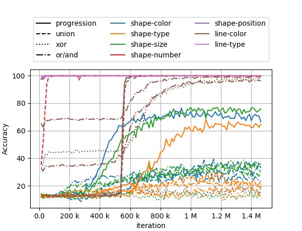
Fig. 6(a), we show the learning progress without L3 , and rules without the multihead loss L3 . However, many rules,
in Fig. 6(b), we show the contribution of L3 when it is especially in the ’shape’ category are not solved well. The
added. It was especially surprising to see that the model addition of the multihead loss immediately and significantly
only started to learn ’line-color’ very late (around 500K it- increases the performance on all rules.
erations) but did it very fast (within 50K iterations for ’pro-
Since training took a long time and we measured only
gression’ and ’union’). The model is able to learn numerous
after each epoch, the plot doesn’t show the progress in the
12(a) (b)
Figure 6. Accuracy for each rule over time. (a) Without L3 . (b) With L3 . It can be seen that during each ’step’, the model is focused at
learning a different subset of tasks. It is also noticeable that the added multihead loss immediately improves the rules that the model was
not able to solve.
early stages of the training, which would show when the
’easier’ tasks have been learned. Future work can focus on
this ’over-time’ analysis and try to explain: (i) ’why are
some rules learned and others not?’, (ii) ’why are some rules
learned faster than others?’, (iii) ’how can the training time
be shortened?’, (iv) ’would the rules that were learned late
also be learned if the easier rules were not present?’.
D. Architecture of each sub-module
We detail each sub-module used in our method in Tab. 7-
10. Since some modules re-use the same blocks, Tab. 6
details a set of general modules.
13Table 6. General modules, with variable number of channels c.
Module layers parameters input output
Conv2D CcK3S1P1 x
BatchNorm
ReLU
ResBlock3(c) Conv2D CcK3S1P1
BatchNorm x0
0
Residual (x, x ) x = x + x0
00
ReLU
Conv2D CcK3S1P1 x
BatchNorm
ReLU
Conv2D CcK3S1P1
BatchNorm x0
DResBlock3(c)
Conv2D CcK1S2P0 x
BatchNorm xd
0
Residual (xd , x ) x = xd + x0
00
ReLU
Conv2D CcK1S1P0 x
BatchNorm
ReLU
ResBlock1(c) Conv2D CcK1S1P0
BatchNorm x0
Residual (x, x0 ) x00 = x + x0
ReLU
Table 7. Encoders Eh , Em , El
Module layers parameters input output
Conv2D C32K7S2P3 I1
BatchNorm
ReLU
Eh
Conv2D C64K3S2P1
BatchNorm
ReLU e1h
Conv2D C64K3S2P1 e1h
BatchNorm
ReLU
Em
Conv2D C128K3S2P1
BatchNorm
ReLU e1m
Conv2D C128K3S2P1 e1m
BatchNorm
ReLU
El
Conv2D C256K3S2P1
BatchNorm
ReLU e1l
14Table 8. Relation networks RNh , RNm , RNl
Module layers parameters input output
Conv2D C64K3S1P1 (e1h , e2h , e3h )
ResBlock3 C64
RNh ResBlock3 C64
Conv2D C64K3S1P1
BatchNorm rh1
Conv2D C128K3S1P1 (e1m , e2m , e3m )
ResBlock3 C128
RNm ResBlock3 C128
Conv2D C128K3S1P1
1
BatchNorm rm
Conv2D C256K1S1P0 (e1l , e2l , e3l )
ResBlock1 C256
RNl ResBlock1 C256
Conv2D C256K1S1P0
BatchNorm rl1
Table 9. Bottlenecks Bh , Bm , Bl
Module layers parameters input output
DResBlock3 C128 bh
Bh
DResBlock3 C128
AvgPool2D vh
DResBlock3 256 bm
Bm
DResBlock3 C128
AvgPool2D vm
Conv2D C256K1S1P0 bl
BatchNorm
Bl
ReLU
ResBlock1 C128 vl
Table 10. MLP
Module layers parameters input output
Linear C256 (vh , vm , vl )
BatchNorm
ReLU
Linear C128
M LP
BatchNorm
ReLU
Linear C1
Sigmoid p(y = 1|I a , IC )
15You can also read