Signal Temporal Logic Synthesis as Probabilistic Inference
←
→
Page content transcription
If your browser does not render page correctly, please read the page content below
Signal Temporal Logic Synthesis as Probabilistic Inference
                                                                              Ki Myung Brian Lee, Chanyeol Yoo and Robert Fitch

                                            Abstract— We reformulate the signal temporal logic (STL)                    We then present three approximate methods for computing
                                         synthesis problem as a maximum a-posteriori (MAP) inference                 the probability of satisfaction of RSTL formulae. Incorpo-
                                         problem. To this end, we introduce the notion of random                     rating these methods, we implement synthesis using GPU-
                                         STL (RSTL), which extends deterministic STL with random
                                         predicates. This new probabilistic extension naturally leads to             accelerated gradient ascent and output the most probable
                                                                                                                     sequence of control actions to satisfy the given specification.
arXiv:2105.06121v1 [cs.RO] 13 May 2021

                                         a synthesis-as-inference approach. The proposed method allows
                                         for differentiable, gradient-based synthesis while extending the               To evaluate our method, we report empirical results that
                                         class of possible uncertain semantics. We demonstrate that the              illustrate correctness, convergence, and scalability properties.
                                         proposed framework scales well with GPU-acceleration, and                   Further, our method inherits the benefits of gradient-based
                                         present realistic applications of uncertain semantics in robotics
                                         that involve target tracking and the use of occupancy grids.                MPC, including the anytime property and predictable com-
                                                                                                                     putation time per iteration.
                                                                 I. I NTRODUCTION                                       To demonstrate practical use in common robotics sce-
                                                                                                                     narios, we provide case studies involving target search and
                                            Temporal logic is a promising tool for robotics applica-                 occupancy grids. These examples show that desirable be-
                                         tions and explainable AI in that it can be used to repre-                   haviour naturally arises, such as prioritising targets whose
                                         sent rich, complex task objectives in the form of human-                    location uncertainty is increasing over targets that are phys-
                                         readable logical specifications. Robot systems equipped with                ically proximate. They also demonstrate the use of complex
                                         the capability to perform STL synthesis can implement                       predicates such occupancy grids which are prevalent robotics
                                         powerful, intuitive command interfaces using STL. We are                    applications. Computational efficiency is shown to parallel
                                         interested in developing STL synthesis for practical, real-                 recent advances in approximate synthesis for deterministic
                                         world applications by viewing the synthesis problem as a                    STL and, importantly, can be further improved through
                                         form of probabilistic inference.                                            additional GPU hardware to enable development of highly
                                            More widespread adoption of formal methods in robot                      capable robot systems.
                                         systems, in our view, is limited by two main factors. First, the               We view the main contribution of this work as a step to-
                                         computational requirements of existing synthesis methods                    wards the feasibility of temporal logic for robotics in practice
                                         are seen as prohibitive. Second, achieving computational                    through the introduction of a new method for synthesis as
                                         efficiency is seen to compromise semantic expressivity.                     probabilistic inference that can accommodate powerful task
                                            The approach we adopt in this paper is to address chal-                  specifications and that has useful performance characteristics.
                                         lenges in both computational efficiency and expressivity                    Our work also provides the basis for interesting theoretical
                                         by viewing STL synthesis as probabilistic inference. This                   extensions that would allow temporal logic specifications
                                         probabilistic approach fits naturally with robotics perception-             to be integrated with estimation methods and belief-based
                                         action pipelines for important information gathering tasks                  planning.
                                         such as search, target tracking, and mapping.
                                                                                                                                         II. R ELATED W ORK
                                            We first present a probabilistic extension of STL, called
                                         random STL (RSTL), that is designed to support synthesis                       To model tasks in uncertain environments, one approach
                                         of robot trajectories that satisfy specifications defined over              is to model the robots’ dynamics as a discrete Markov deci-
                                         uncertain events in the environment. Formally, RSTL extends                 sion process (MDP), where each state is assigned semantic
                                         STL to include uncertain semantic labels. The gain in                       labels with corresponding uncertainty [1–4]. A natural task
                                         expressivity is the capacity to specify tasks in a way that                 specification tool is linear temporal logic (LTL), given which
                                         facilitates robust behaviour in real-world settings; uncertainty            a product MDP [1] is constructed from an automaton and a
                                         that is inherent to practical environments can be anticipated               sequence of actions are found that maximize the probability
                                         explicitly instead of handled reactively. Synthesising tra-                 of satisfaction. These ideas can be extended to the contin-
                                         jectories is a differentiable problem that largely resembles                uous case by judiciously partitioning the environment [5–
                                         previously proposed differentiable measures of robustness for               7]. However, we find that partitioning is computationally
                                         deterministic STL synthesis.                                                prohibitive for online operations in uncertain environments,
                                                                                                                     because any change in belief about the environment would
                                            This research is supported by an Australian Government Research Train-   lead to invalidation and expensive recomputation. Moreover,
                                         ing Program (RTP) Scholarship and the University of Technology Sydney.      the construction of a product MDP is a computationally
                                            Authors are with the University of Technology Sydney, Ul-
                                         timo, NSW 2006, Australia brian.lee@student.uts.edu.au,                     expensive operation, and improving its scalability remains
                                         {chanyeol.yoo, rfitch}@uts.edu.au                                           an open problem.
Signal temporal logic (STL) [8] is defined over continuous       where E ∈ E, and Ψ, Φ are RSTL formulae. ¬ is logical
signals. Unlike in LTL, satisfaction is determined using            negation, ∧ is logical conjunction. U is the temporal operator
continuous-valued robustness [9]. Existing work uses STL to         ‘Until’, and ΦU[t1 ,t2 ] Ψ means Φ must hold true between
specify a task defined over a set of deterministic classes of       time [t1 , t2 ] until Ψ. Other operators such as ∨ (disjunction),
conditions on the environment uncertainty, such as chance           F[t1 ,t2 ] (‘in Future’, i.e., eventually) and G[t1 ,t2 ] (‘Globally’,
constraints or variance limits [10–12]. However, since the          i.e., always) can be derived from the syntax the same way
robustness evaluation is not differentiable, a common ap-           as deterministic STL [8]. The events E will be referred to
proach is to synthesise solutions using mixed integer linear        as ‘event predicates’.
programming (MILP) which scales exponentially with the                 RSTL is random in the sense that, for a given trajectory
size of mission horizon [10, 13]. To address the inherent           X, the satisfaction of an RSTL formula Φ is a Bernoulli
complexity, the robustness metric is approximated to smooth         random event. The probability of satisfaction is the expected
the search space and find a solution using gradient ascent.         rate of satisfaction computed over sampled instances of the
                                                                    event predicates Ê = {e1 , ..., eM } ∼ E:
               III. P ROBLEM F ORMULATION
   Suppose we have a robot with N -dimensional state xt ∈                         P((X, t) |= Φ) = E Sat(X, t, Ê, Φ),                (5)
RN and control actions ut ∈ U, where U is a continuous                                                  Ê∼E
set of admissible control actions. The robot’s dynamics is
uncertain, and is modelled by a discrete-time, continuous-          where Sat(X, t, Ê, Φ) is a deterministic function evaluated
space MDP P(xt+1 | xt , ut ) between t and t + 1, so that           recursively as:
the trajectory distribution over a horizon T is given by:
                                                                              Sat(X, t, Ê, E i ) ≡ ei (xt , t) ∼ P i (xt , t)
                                 T
                                 Y                                           Sat(X, t, Ê, ¬Φ) ≡ ¬Sat(X, t, Ê, Φ)
          P(X | U) = P(x1 )            P(xt+1 | xt , ut ),   (1)
                                 t=1                                     Sat(X, t, Ê, Φ ∧ Ψ) ≡ Sat(X, t, Ê, Φ) ∧ Sat(X, t, Ê, Ψ)
where X ≡ x1 ...xT and U ≡ u1 ...uT .                               Sat(X, t, Ê, ΦU[t1 ,t2 ] Ψ) ≡
   The robot encounters a finite set of random events E =                _            ^
                                                                                                Sat(X, τ2 , Ê, Φ) ∨ Sat(X, τ1 , Ê, Ψ).
{E 1 , ..., E M } (e.g., ‘object detected’), whose probability of
                                                                      τ1 ∈t+[t1 ,t2 ] τ2 ∈t1 +[0,τ1 ]
occurrence depends on robot’s state xt and time t. We are                                                                    (6)
interested in finding control actions U∗ that maximises the         Note that ei (xt , t) ∈ {0, 1} is a sample from E i at robot
probability of satisfying a task Φ defined over E (e.g. ‘detect     state xt and time t.
all objects’). Namely, this is a synthesis problem:
Problem 1 (Synthesis). Given the uncertain dynamics (1),            B. STL Synthesis as Inference
and a task specification Φ over a set of random events E with
                                                                       Since both task satisfaction and robot dynamics are prob-
probability of satisfaction P ((X, t) |= Φ), find an optimal
                                                                    abilistic, it is natural to ask if Problem 1 can be solved
sequence of controls U∗ such that the trajectory X max-
                                                                    solely within the realm of probability theory. This is achieved
imises the probability of satisfying Φ over time horizon T :
                                                                    by the control-as-inference paradigm [14, 15], which has
              U∗ = argmax P ((X, t) |= Φ) ,                  (2)    been shown to not only encompass existing optimal control
                       U∈UT                                         problems, but also to enable new approaches. We follow a
with respect to time t = 1.                                         similar development and present an inference formulation of
                                                                    Problem 1.
   IV. STL S YNTHESIS AS P ROBABILISTIC I NFERENCE
                                                                       In this formulation, the problem is modelled by the joint
  In this section, we first introduce random signal temporal        distribution among task satisfaction, robot trajectory, and
logic (RSTL), a probabilistic extension of STL that allows          control actions:
specification of tasks Φ over random events E. We then
present a probabilistic inference formulation of Problem 1.                   P(Φt , X, U) = P(Φt | X)P(X | U)P(U),                   (7)
A. Random STL Formulae
                                                                    where P(Φt | X) ≡ P((X, t) |= Φ) denotes the probability
   We model the random events E = {E 1 , ..., E M } as (not         satisfaction of Φ given X with respect to time t.
necessarily independent) Bernoulli random variables that
                                                                       Here, P(U) is our prior belief on what the control actions
are dependent on robot’s state and time, with conditional
                                                                    should be, and is representative of the admissible control
probability of occurrence:
                                                                    space U in the synthesis formulation. For example, if P(U)
                P(E i = 1 | xt , t) = P i (xt , t).          (3)    is a zero-mean Gaussian prior, it is equivalent to penalising
                                                                    quadratic control cost. The prior can derive from other
In other words, each E i is a Bernoulli random field over
                                                                    knowledge, e.g., an imitation-learnt prior as [16] does for
RN × R+ . Given a set of random events E, the syntax of an
                                                                    optimal control.
RSTL formula Φ is given by:
                                                                       A balance between admissibility and probability of sat-
             Φ := E | ¬Φ | Φ ∧ Ψ | ΦU[t1 ,t2 ] Ψ,            (4)    isfaction is captured by the posterior probability of control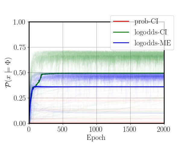
actions given that the task is satisfied:                              where A and B are independent Bernoulli random variables,
                                                                       and lse is the log-sum-exp function:
      P(U | Φt ) ∝ P(Φt | U)P(U)                                                                              X
                        Z
                                                                 (8)                 lse(L1 , ..., LN ) = log   exp Li .   (14)
                 = P(U) P(Φt | X)P(X | U)dX,                                                                       i
                                                                       A series of disjunction operations (13) is then:
We thus pose Problem 1 as a maximum a posteriori (MAP)                                     !
inference problem:                                                                  _               X       X
                                                                                L       Ai = log        exp      L(Aj ),            (15)
Problem 2 (Inference). Given the dynamic model (1) and                               i∈I               J∈2I        j∈J
an RSTL task specification Φ, find the MAP control actions             where 2I denotes the power set of I.
U∗ given the robot’s trajectory satisfies Φ with respect to t:            Computing log-sum-exp over sum of all subsets is clearly
                  U∗ = argmax P(U | Φt ).                        (9)   cumbersome. We avoid such computation by using the re-
                            U                                          lationship between elementary symmetric polynomials and
          V. A PPROXIMATE G RADIENT A SCENT                            monic polynomials. Observe that the summations over j ∈ J
                                                                       can be taken out of the exponential as products. Then, we
   In this section, we first present approximate methods that          have all elementary symmetric polynomials over Ai less 1.
allow analytical evaluation of (5). We then present a gradient-        We thus arrive at a more compact expression:
ascent scheme on these approximate evaluations.                                      !                                !
                                                                               _              Y
A. Conditional Independence Approximation                                   L     Ai = log        1 + exp L(Ai ) − 1 .        (16)
                                                                                i                  i
   To compute (5) analytically, we observe that (5) applies               Now, the CI computation rules in the log-odds domain are
logical operations to samples from Bernoulli random vari-              given as follows:
ables. A convenient approximation is the product relation
for independent Bernoulli random variables A and B:                    Definition 2 (CI-approximate log-odds). Given an RSTL
                                                                       formula Φ, the CI-approximation of log-odds of satisfaction
                  P(A ∧ B) = P(A)P(B).                          (10)   L(Φt | X) is calculated by:
   Technically, the product relation holds true if the operands                  L(Eti | X) ≡ log P i (X, t) − log(1 − P i (X, t))
are conditionally independent given X. The conditionally                     L(¬Φt | X) ≡ −L(Φt | X)
independent (CI)-approximation is defined by one of the                               !                                   !
                                                                             _                Y
authors [17] as follows:                                                   L   Φit | X ≡ log     (1 + exp L(Φit | X)) − 1)
                                                                                i                       i
Definition 1 (CI-approximation [17]). Given an RSTL for-                                               Y
mula Φ, the CI-approximation of P(Φt | x) is defined by:               L((F[t1 ,t2 ] Φ)t | X) ≡ log           1 + exp L(Φτ | X − 1 .
                                                                                                  τ ∈t+[t1 ,t2 ]
                 P(Eti | X) ≡ P i (X, t)                                                                                            (17)
               P(¬Φt | X) ≡ 1 − P(Φt | X)
                ^           Y                                             It is interesting to note that the proposed computation
              P( Φit | X) ≡    P(Φit | X)                       (11)   rules for probability of satisfaction exhibits strong similar-
                  i                 i
                                        Y                              ities to existing work on deterministic STL synthesis and
        P((G[t1 ,t2 ] Φ)t | X) ≡                    P(Φτ | X)          model checking [8, 18–20]. In the log-odds domain, certain
                                   τ ∈t+[t1 ,t2 ]                      satisfaction (i.e. probability of 1) translates to ∞, certain dis-
                                                                       satisfaction is −∞, and absolute uncertainty (i.e. probability
B. Log-odds Transform                                                  of 0.5) is 0, which are the behaviours of spatial robustness
   The output range for CI-approximation of P (11) is [0, 1]           measure for deterministic STL introduced in [8]. Further,
since it computes probability. This can lead to numerical in-          the log-sum-exp function has been used in deterministic
stability, and gradient ascent often leads to poor convergence.        STL synthesis [18, 19] as a smooth approximation of the
A natural re-parameterisation for Bernoulli random variables           maximum function. Finally, A similar expression to (16)
is the log-odds:                                                       was presented in [20] as an alternative robustness measure
                                     P(A)                              for deterministic STL. The authors report encouragement of
                      L(A) = log           ,                    (12)   repeated satisfaction, which is consistent with the probability
                                     P(¬A)
                                                                       of disjunction increasing with increasing probability of the
   It can be shown with some algebraic manipulations that              disjuncts.
re-writing the CI rule for pairwise disjunction ∨ in (11) in              Given that the approaches that do not encourage repeated
terms of log-odds leads to:                                            satisfaction [18, 19] still report acceptable results, we con-
                 P(A)P(B) + P(¬A)P(B) + P(A)P(¬B)                      sider the following approximation for disjunction:
L(A ∨ B) = log                                                             L(A ∨ B) ≈ lse(L(A), L(B)))
                              P(¬A)P(¬B)
           = lse(L(A), L(B), L(A) + L(B)),                                                P(A)P(¬B) + P(¬A)P(B)                     (18)
                                                                                    = log                       .
                                              (13)                                               P(¬A)P(¬B)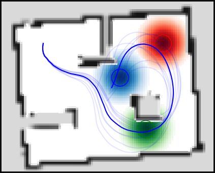
analytical gradients can be computed easily using autograd
frameworks such as Tensorflow [21] or PyTorch [22, 23].
Therefore, we do not present the expressions here.
VI. E MPIRICAL A NALYSIS
We evaluate the practical performance characteristics of
the proposed method. We first demonstrate that the proposed
CI (17) and ME (19) methods reasonably approximate the
ground truth (5). We then examine the convergence charac-
teristics of the gradient ascent (22) solution, and demonstrate
(a) F (A) ∧ F (B) (b) F (A ∧ F (B))
the computational benefits of GPU acceleration.
Fig. 1. Comparison of the CI (green) and ME (blue) approximation results
against MC estimates (‘Empirical’). CI is exact for F (A)∧F (B), while ME A. Quality of Approximation
underestimates. For F (A∧F(B)), the error increases, but not significantly.
Naive method’s result showed numerically insignificant difference to CI, and In this section, we evaluate whether the CI and ME
is omitted. approximations compute the probability of satisfaction ac-
curately. Because the CI computation rule assumes indepen-
dence amongst operands, we expect it to be exact if 1) all
This ignores repeated satisfaction by omitting the P(A)P(B)
predicates are conditionally independent; 2) each predicate is
term from the numerator of (13). Meanwhile, there is a
independent across time and space; and 3) only one operator
potential numerical benefit that log-sum-exp can be com-
uses each predicate. For example, assuming 1) and 2) hold,
puted numerically stably with the so-called log-sum-exp
we expect the CI rule to be exact on FA ∧ FB, but not
trick, while the product in (16) may underflow. We thus
F(A ∧ FB), because the disjuncts of the outer F operator
define the mutually exclusive (ME) approximation as follows.
are not independent. The ME computation rules (19) will not
Definition 3 (ME approximation). Given an RSTL formula be exact in any case.
Φ, the ME approximation of L(Φt | X) is calculated by: We validate these hypotheses by comparing against a
1000-sample Monte Carlo (MC) approximation of RSTL
L(Eti | X) ≡ log P i (X, t) − log(1 − P i (X, t))
probability of satisfaction (5). We used the trajectories from
L(¬Φt | X) ≡ −L(Φt | X) the first 2000 gradient ascent steps generated from the
L(Φt ∨ Ψt | X) ≡ lse(L(Φt | x), L(Ψt | X)) (19) target search scenario (Fig. 4). For simplicity, we evaluated
L((FI Φ)t | X) ≡ log
X
exp L(Φτ | X). each predicates’ marginal probability independently before
τ ∈t+I
sampling, so that the first two conditions of exactness hold.
In Fig. 1a, CI (green) and ME (blue) results are compared
C. Synthesis with Gradient-Ascent against the MC estimate for FA ∧ FB. It can be seen that
the CI method matches the MC result as expected, while
With the probability or log-odds of satisfaction computed,
ME consistently underestimates. This is expected, because
we synthesise a MAP control sequence U∗ that maximises
ME does not account for multiple satisfaction.
the posterior probability. We use Jensen’s inequality to bound
Figure 1b shows comparison for F(A ∧ FB). As FB is
the log of posterior probability (9):
double-counted by the outer F, CI and ME tend to over-
log P(U | Φt ) ≥ E [log P(Φt | X))] + log P(U). estimate, but not by much. ME continues to underestimate,
X∼P(X|U)
(20) and CI matches the MC closely, showing that CI and ME
Subsequently, we maximize the lower bound: are reasonable approximations for practical applications.
U∗ = argmax E [log P(Φt | U)]+log P(U). (21) B. Convergence
U X∼P(X|U)
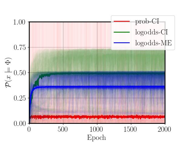
Gradient-based methods cannot guarantee globally optimal
The maximisation is done by gradient ascent on (21). solutions unless the objective is convex. We analyse the
Because the expectation in (21) is intractable, we replace convergence characteristics of the proposed computation
it with an empirical mean over a Ns number of trajectory rules in the target search scenario (Fig. 4). We randomly
samples, so that the i-th gradient ascent step is: generated 100 initial conditions from the control prior P(U),
and ran the gradient ascent step for 2000 iterations, with
1 X ∂
Ûi+1 = Ûi + [log P(Φt | Xj1:T (Ûi ))+log P(Ûi )], Ns = 1, 50, 100 number of trajectory samples.
Ns j ∂ Ûi Figure 2 shows the probability of satisfaction over gradient
(22) ascent steps for naive CI ((11), red), log-odds CI ((17), green)
where Ûi+1 = ûi1 ...ûiT . Each trajectory sample Xj (Ûi ) and log-odds ME ((19), blue) methods with varying number
is obtained by propagating the dynamic model (1) forward of trajectory samples Ns . It can be seen that while log-odds
in time including actuation uncertainty. Note that, as long as CI and ME methods find global and local optima, the naive
the predicates’ distributions and the dynamic model are dif- CI method does not find any. The naive CI method’s failure
ferentiable, so is (22). For both CI and ME approximations, is attributed to the computation rules (11) being bounded to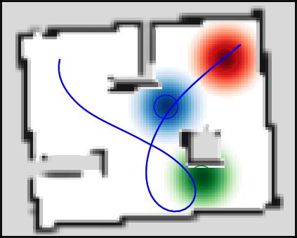
(a) Ns = 1 (b) Ns = 50 (c) Ns = 100
Fig. 2. Comparison of convergence with number of trajectory samples. Solid lines are medians.
all changes. The result shows that the computation time
with GPU is significantly lower than that with CPU, and
that using a GPU leads to 4-fold improvement in scalability.
This demonstrates that the proposed gradient ascent method
benefits from GPU acceleration.
VII. C ASE S TUDIES
We demonstrate two example cases that illustrate the
benefit of using RSTL for task specification in uncertain
environments. The proposed gradient ascent method was im-
Fig. 3. Comparison of average computation time per gradient ascent step plemented in Tensorflow [21]. For all examples, we consider
between combinations of CPU (red) and GPU (green) with CI (upward
triangle and ME (downward triangle). GPU shows 4-fold improvement in a robot described by a bicycle dynamic model:
scalability. Variance was in the order of 10−4 for all configurations.
ẋt Vt cos θt
ẋt = ẏt = Vt sin θt , (23)
[0, 1] range, which causes numerical errors to build up. Note θ̇t ωt + t
that log-odds ME reports lower probability of satisfaction where t ∼ N (0, σu ) is white Gaussian noise. The control
due to its underestimation property, but we found that the >
inputs are ut = Vt ωt .
resulting trajectories were still similar.
With increasing Ns , the variance in probability of satis- A. 2D Target Search
faction is decreased. In practice, this means the generated We consider a 2D target search scenario, where a robot
plan will more reliably account for state uncertainty, which is tasked with detecting possibly moving targets in the
is useful for, e.g., the collision avoidance scenario in Fig. 5. environment: Tom and Jerry. Jerry, as usual, is moving with
increasing uncertainty, while Tom is stationary with high
C. Computation Time certainty. Figure 4 depicts an example where the mean paths
The results in Sec. VI-B illustrate that it is important to for Tom and Jerry are shown in green and red. The growing
use multiple initial conditions and more trajectory samples uncertainty over time is shown around the mean. Note that
to ensure reliable operation. However, this would inevitably since Tom (in green) is known to be stationary, its uncertainty
increase the computation time as well. does not grow over time. The robot starts at [0, 0]> .
GPU acceleration is a prominent means to circumvent the The task of finding Tom and Jerry can be expressed using
issue of computation time, but not all algorithms benefit from RSTL as Φ = F(DTom ) ∧ F(DJerry ) (i.e., ‘eventually detect
GPU acceleration. To determine if our proposed methods Tom and eventually detect Jerry’).
benefit from GPU acceleration, we compare the computation We model the events DTom and DJerry as follows. If the
time per gradient ascent step of our Tensorflow [21] imple- location is known, the robot detects Tom and Jerry with
mentation between GPU and CPU. We used all combinations likelihood modelled by:
between Ns = 1, 10, 50, 100 and Nu = 1, 10, 50, 100, and
||xt − zt ||2
computed the mean over 1000 gradient ascent steps. We used P(Dt | xt , zt ) = PD exp 2 , (24)
a desktop with CPU (Intel i5-9500) and a GPU (NVIDIA 2rD
RTX2060) to conduct the experiment. where zt is the location of the target, rD is the radius of
Figure 3 shows the computation time with varying number detection, and PD controls the peak.
of initial conditions Nu and the number of state samples Ns . Tom and Jerry are modelled by a constant acceleration
We found that the total number of samples Nu ×Ns explains model, which is a linear Gaussian system. The mean z̄a,b
t andand then Jerry later. This is because the uncertainty of Jerry
grows unlike Tom, and the optimal trajectory should detect
Jerry first before its uncertainty grows. This demonstrates
that RSTL naturally reasons over uncertainty.
B. Complex Missions in an Indoor Environment
Consider a nursing robot in an indoor environment, mod-
elled as an occupancy grid O such that Oi,j is the probability
of obstacle occupancy. Collision with an obstacle is modelled
(a) t = 15 (b) t = 10 by an interpolation:
X
P(O | xt ) = Kij (xt )Oi,j , (26)
i,j
where Kij (x) denotes the interpolant.
The robot cares for two patients, Rob and Bob. The doctor
asks the robot to avoid obstacles, and to never visit any of
the patients before visiting the sanitising station, which can
be written as an RSTL formula:
Φ1 = (¬(DRob ∨ DBob )UDSan ) ∧ G(¬O), (27)
(c) t = 45 (d) t = 45
Fig. 4. A 2D target search scenario. The robot (blue) is tasked with where DRob , DBob , and DSan are distributed as per (25).
detecting both Tom (Green) and Jerry (Red). The global optimum with Now, in addition to the previous command, the doctor asks
P(Φ | x) ≈ 0.7 (left column) is to detect Jerry before uncertainty grows.
A local optimum with P(Φ | x) ≈ 0.5 (right column) prefers Tom, who is the robot to visit the two patients:
closer. Circles show 1-covariance bound.
Φ2 = F(DRob ) ∧ F(DBob ) ∧ Φ1 . (28)
We created an occupancy grid from a realistic dataset
commonly used in perception research [24, 25], and com-
pared the results with low (10− 4rads−1 ) and high (σu =
0.1rads−1 ) actuation uncertainty. The results are shown in
Fig. 5. In both cases, the generated trajectory is correct,
visiting the sanitising station first, and then the two patients.
Interestingly, the trajectory changes drastically when control
noise increases. The path with small control noise in Fig. 5a
(a) σu = 10−4 (b) σu = 0.1 is aggressively close to the wall, whereas the path with
Fig. 5. Results for complex indoor mission. The robot’s (blue) task
control noise in Fig. 5b is more conservative in that the
is a conjunction of ‘never visit Rob (red) or Bob (blue) before visiting robot keeps distance away from the wall by manoeuvring
sanitising station (green), and avoid obstacles (grey colormap)’, and ’visit around the obstacle. This demonstrates that the proposed
Rob (red) and Bob (blue)’. With higher actuation uncertainty σu , the
trajectory becomes further from the walls. Solid lines are the robot’s nominal
probabilistic formulation enables risk-averse behaviour in
trajectory in the absence of noise. Transparent blue lines are the noised STL synthesis, a crucial property for practical applications.
samples used during synthesis. The start location is top-left corner.
VIII. C ONCLUSION
Σa,b are propagated given the robots’ belief at t = 0 using We have presented a probabilistic inference perspective on
t
the standard prediction equations. The marginal probability STL synthesis based on RSTL and corresponding algorithms.
of detection accounting for their uncertainty is given by: Our method exhibits appealing computational and expressiv-
ity characteristics that suit practical robotics applications. We
||xt − z̄t ||2
Z
anticipate that the inference formulation of STL synthesis
P(Dt | xt ) = exp N (z̄t , Σzt )dzt
2rd2 (25) presented in this paper will accelerate the development
√ of explainable AI techniques through seamless integration
N N z 2
= 2π rd N (z̄t , Σt + rd I),
between formal methods and machine learning techniques as
where N (z̄t , Σzt ) is the multivariate Gaussian PDF. did the optimal control-as-inference paradigm [14, 15]. Many
Figure 4 shows global and local optima found using the avenues of future work arise from our results; one of the
log-odds CI computation rule (17). It can be seen that the most exciting is integration with estimation methods [26–28]
global optimum (Figs. 4a and 4c) is to detect Jerry first at t = that would allow multi-robot systems to augment or replace
15 (Fig. 4a), and to return to Tom at t = 45 (Fig. 4c), while explicit communication for behaviour coordination with tra-
the local optimum is to detect Tom first at t = 10 (Fig. 4b) jectory predictions derived from specifications [29, 30].R EFERENCES F. d’Alché Buc, E. Fox, and R. Garnett, Eds. Curran Associates, Inc.,
2019, pp. 8024–8035.
[1] X. Ding, S. L. Smith, C. Belta, and D. Rus, “Optimal control of [23] K. Leung, N. Aréchiga, and M. Pavone, “Back-propagation through
Markov decision processes with linear temporal logic constraints,” signal temporal logic specifications: Infusing logical structure into
IEEE Trans. Automat. Contr., vol. 59, no. 5, pp. 1244–1257, 2014. gradient-based methods,” in Algorithmic Foundation of Robotics XIV,
[2] S. Bharadwaj, M. Ahmadi, T. Tanaka, and U. Topcu, “Transfer entropy S. M. LaValle, M. Lin, T. Ojala, D. Shell, and J. Yu, Eds. Springer,
in MDPs with temporal logic specifications,” in Proc. of IEEE CDC, 2021, vol. 17, pp. 432–449.
2018, pp. 4173–4180. [24] B. Lee, C. Zhang, Z. Huang, and D. D. Lee, “Online continuous
[3] C. Yoo, R. Fitch, and S. Sukkarieh, “Probabilistic temporal logic for mapping using Gaussian process implicit surfaces,” in Proc. of IEEE
motion planning with resource threshold constraints,” Proc. of RSS, ICRA, 2019, pp. 6884–6890.
2012. [25] L. Wu, K. M. B. Lee, L. Liu, and T. Vidal-Calleja, “Faithful Euclidean
[4] ——, “Provably-correct stochastic motion planning with safety con- distance field from log-Gaussian process implicit surfaces,” IEEE
straints,” in Proc. of IEEE ICRA, 2013, pp. 981–986. Robot. and Automat. Lett., vol. 6, no. 2, pp. 2461–2468, 2021.
[5] T. Wongpiromsarn, U. Topcu, N. Ozay, H. Xu, and R. M. Murray, [26] K. M. B. Lee, C. Yoo, B. Hollings, S. Anstee, S. Huang, and
“TuLiP: A software toolbox for receding horizon temporal logic R. Fitch, “Online estimation of ocean current from sparse GPS data for
planning,” in Proc. of HSCC, 2011, pp. 313–314. underwater vehicles,” in Proc. of IEEE ICRA, 2019, pp. 3443–3449.
[6] C. Yoo, R. Fitch, and S. Sukkarieh, “Online task planning and control [27] G. Best and R. Fitch, “Bayesian intention inference for trajectory
for fuel-constrained aerial robots in wind fields,” Int. J. of Robot. Res., prediction with an unknown goal destination,” in Proc. of IROS, 2015,
vol. 35, no. 5, pp. 438–453, 2016. pp. 5817–5823.
[7] J. J. H. Lee, C. Yoo, S. Anstee, and R. Fitch, “Hierarchical planning [28] N. Rhinehart, R. McAllister, K. Kitani, and S. Levine, “PRECOG:
in time-dependent flow fields for marine robots,” in Proc. of IEEE Prediction conditioned on goals in visual multi-agent settings,” in Proc.
ICRA, 2020, pp. 885–891. of Int. Conf. on Comput. Vision, October 2019.
[8] A. Donzé, “On signal temporal logic,” in Runtime Verification, [29] K. M. B. Lee, F. Kong, R. Cannizzaro, J. L. Palmer, D. Johnson,
A. Legay and S. Bensalem, Eds. Berlin, Heidelberg: Springer Berlin C. Yoo, and R. Fitch, “An upper confidence bound for simultaneous
Heidelberg, 2013, pp. 382–383. exploration and exploitation in heterogeneous multi-robot systems,” in
[9] J. V. Deshmukh, A. Donzé, S. Ghosh, X. Jin, G. Juniwal, and S. A. Proc. of IEEE ICRA, 2019.
Seshia, “Robust online monitoring of signal temporal logic,” Formal [30] G. Best, O. M. Cliff, T. Patten, R. R. Mettu, and R. Fitch, “Dec-MCTS:
Methods in Syst. Des., pp. 5–30, 2017. Decentralized planning for multi-robot active perception,” The Int. J.
[10] D. Sadigh and A. Kapoor, “Safe control under uncertainty with prob- of Robot. Res., vol. 38, no. 2-3, pp. 316–337, 2019.
abilistic signal temporal logic,” in Proc. of RSS, AnnArbor, Michigan,
June 2016.
[11] M. Tiger and F. Heintz, “Incremental reasoning in probabilistic signal
temporal logic,” Int. J. Approx. Reason., vol. 119, pp. 325–352, April
2020.
[12] C.-I. Vasile, K. Leahy, E. Cristofalo, A. Jones, M. Schwager, and
C. Belta, “Control in belief space with temporal logic specifications,”
in Proc. of IEEE CDC, 2016, pp. 7419–7424.
[13] V. Raman, A. Donzé, M. Maasoumy, R. M. Murray, A. Sangiovanni-
Vincentelli, and S. A. Seshia, “Model predictive control with signal
temporal logic specifications,” in Proc. of IEEE CDC, 2014, pp. 81–
87.
[14] H. J. Kappen, V. Gómez, and M. Opper, “Optimal control as a
graphical model inference problem,” Mach. learn., vol. 87, no. 2, pp.
159–182, 2012.
[15] S. Levine, “Reinforcement learning and control as probabilistic infer-
ence: Tutorial and review,” arXiv preprint arXiv:1805.00909, 2018.
[16] N. Rhinehart, R. McAllister, and S. Levine, “Deep imitative models
for flexible inference, planning, and control,” in Proc. of ICLR, April
2020.
[17] C. Yoo and C. Belta, “Control with probabilistic signal temporal logic,”
arXiv preprint arXiv:1510.08474, 2015.
[18] L. Lindemann and D. V. Dimarogonas, “Control barrier functions for
signal temporal logic tasks,” IEEE Contr. Syst. Lett., vol. 3, no. 1, pp.
96–101, 2019.
[19] I. Haghighi, N. Mehdipour, E. Bartocci, and C. Belta, “Control
from signal temporal logic specifications with smooth cumulative
quantitative semantics,” in Proc. of IEEE CDC, 2019, pp. 4361–4366.
[20] N. Mehdipour, C. Vasile, and C. Belta, “Arithmetic-geometric mean
robustness for control from signal temporal logic specifications,” in
Proc. of IEEE ACC, 2019, pp. 1690–1695.
[21] M. Abadi, A. Agarwal, P. Barham, E. Brevdo, Z. Chen, C. Citro,
G. S. Corrado, A. Davis, J. Dean, M. Devin, S. Ghemawat,
I. Goodfellow, A. Harp, G. Irving, M. Isard, Y. Jia, R. Jozefowicz,
L. Kaiser, M. Kudlur, J. Levenberg, D. Mane, R. Monga,
S. Moore, D. Murray, C. Olah, M. Schuster, J. Shlens, B. Steiner,
I. Sutskever, K. Talwar, P. Tucker, V. Vanhoucke, V. Vasudevan,
F. Viégas, O. Vinyals, P. Warden, M. Wattenberg, M. Wicke,
Y. Yu, and X. Zheng, “TensorFlow: Large-scale machine learning on
heterogeneous systems,” 2015. [Online]. Available: http://tensorflow.
org/
[22] A. Paszke, S. Gross, F. Massa, A. Lerer, J. Bradbury, G. Chanan,
T. Killeen, Z. Lin, N. Gimelshein, L. Antiga, A. Desmaison, A. Kopf,
E. Yang, Z. DeVito, M. Raison, A. Tejani, S. Chilamkurthy, B. Steiner,
L. Fang, J. Bai, and S. Chintala, “Pytorch: An imperative style, high-
performance deep learning library,” in Advances in Neural Information
Processing Systems 32, H. Wallach, H. Larochelle, A. Beygelzimer,You can also read