Sinkhole susceptibility mapping: a comparison between Bayes-based machine learning algorithms - Universidad de Zaragoza
←
→
Page content transcription
If your browser does not render page correctly, please read the page content below

Sinkhole susceptibility mapping: a comparison between Bayes-based machine learning
                                                    algorithms

Kamal Taheri1, Himan Shahabi2, *, Kamran Chapi3, Ataollah Shirzadi3, Francisco Gutiérrez4,
                                                Khabat Khosravi5

            1
                Karst Research and Study Office of Western Iran, Kermanshah Regional Water Authority,
                                                 Kermanshah, Iran
    2
     Department of Geomorphology, Faculty of Natural Resources, University of Kurdistan, Sanandaj,
                                                        Iran
3
    Department of Rangeland and Watershed Management, Faculty of Natural Resources, University of
                                             Kurdistan, Sanandaj, Iran
        4
            Earth Science Department, Edificio Geológicas, Universidad de Zaragoza, Zaragoza, Spain
        5
            Department of Watershed Sciences Engineering, Faculty of Natural Resources, University of
                         Agricultural Science and Natural Resources of Sari, Mazandaran, Iran

Corresponding Author: Himan Shahabi, Department of Geomorphology, Faculty of Natural
*

Resources, University of Kurdistan, Sanandaj, Iran, E-mail: h.shahabi@uok.ac.ir                 Tel: +98-
9186658739

This article has been accepted for publication and undergone full peer review but has not
been through the copyediting, typesetting, pagination and proofreading process which may
lead to differences between this version and the Version of Record. Please cite this article as
doi: 10.1002/ldr.3255

                                               This article is protected by copyright. All rights reserved.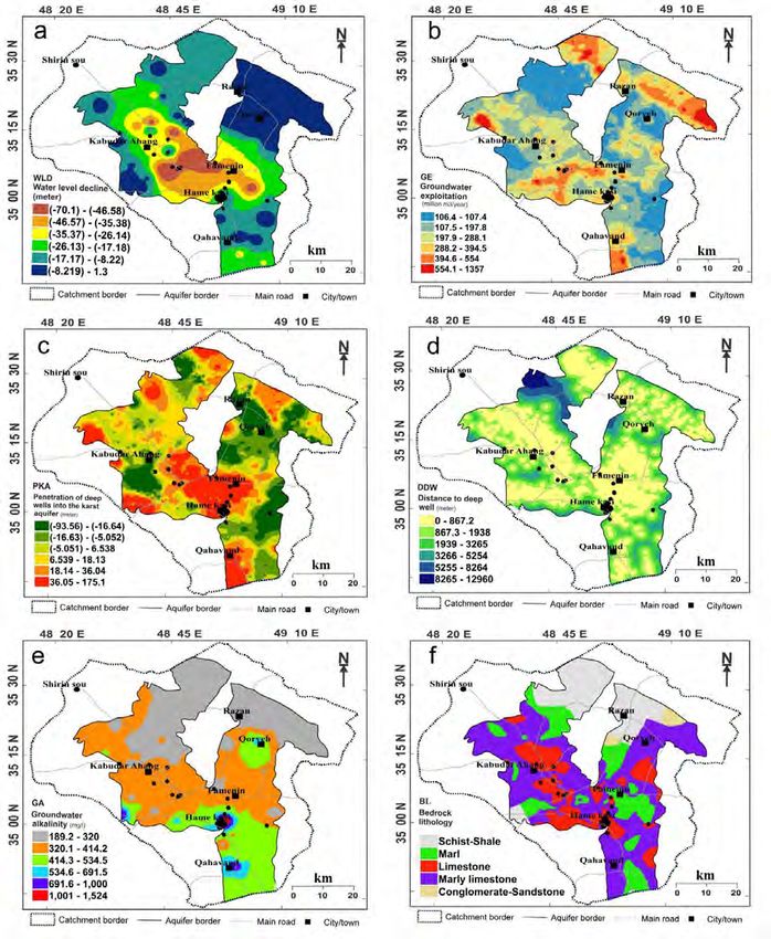
ABSTRACT
Land degradation has been recognized as one of the most adverse environmental impacts
during the last century. The occurrence of sinkholes is increasing dramatically in many
regions worldwide contributing to land degradation. The rise in the sinkhole frequency is
largely due to human-induced hydrological alterations that favour dissolution and subsidence
processes. Mitigating detrimental impacts associated with sinkholes requires understanding
different aspects of this phenomenon such as the controlling factors and the spatial
distribution patterns. This research illustrates the development and validation of sinkhole
susceptibility models in Hamadan Province, Iran, where a large number of sinkholes are
occurring under poorly understood circumstances. Several susceptibility models were
developed with a training sample of sinkholes, a number of conditioning factors and four
different statistical approaches: Naïve Bayes (NB), Bayes Net (BN), Logistic Regression
(LR), and Bayesian Logistic Regression (BLR). Ten conditioning factors were initially
considered. Factors with negligible contribution to the quality of predictions, according to the
information gain ratio (IGR) technique, were discarded for the development of the final
models. The validation of susceptibility models, performed using different statistical indices
and ROC-curves, revealed that the BN model has the highest prediction capability in the
study area. This model provides reliable predictions on the future distribution of sinkholes,
which can be used by watershed and land-use managers for designing hazard and land-
degradation mitigation plans.

Keywords: Sinkhole, Naïve Bayes, Bayes Net, Logistic Regression, Iran

                                     This article is protected by copyright. All rights reserved.
INTRODUCTION
Land degradation is a major problem worldwide, especially in developing countries, due
mainly to the improper use of land, soil and water resources (Jafari & Bakhshandehmehr,
2016; Symeonakis et al., 2016). Land degradation is generally attributed to human activities
that cause detrimental effects upon the land, typically involving reduction in its productive
capacity (Minaei et al., 2018). Sinkholes are considered as the most characteristic landform in
karst terrains, which represent around 20% of the continental surface (Ford & Williams,
2013). Sinkholes, like other geohazards, are generally viewed as natural phenomena rather
than as a land-degradation agent. However, extensive literature on the subject reveals that a
large proportion of the new sinkholes are human-induced (e.g., Parise, 2013; Bui et al.,
2018b). Anthropogenic activities such as groundwater withdrawal, irrigation, dewatering for
mining or diversion of river flow, are increasing the frequency of sinkholes in many regions
worldwide (Filippi & Bosák, 2013; Parise, 2013; Vattano et al., 2013; Gutiérrez et al., 2014;
Chen et al., 2017; Tien Bui et al., 2018). The formation of sinkholes involves the reduction of
agricultural land, may significantly compromise safety, cause severe damage to
infrastructure, and in extreme cases may result in the abandonment of agricultural areas and
irrigation plans (Gunn, 2004; Hyland, 2005). Overall, the impacts associated with sinkholes
are particularly severe in arid areas, where the exploitation of water resources for irrigation
leads to rapid hydrological changes (e.g., water-table decline, sharp increase in water
infiltration) that contribute to trigger sinkholes. In many of these areas, groundwater over-
exploitation and the consequent decline in the water table, together with the onset of
irrigation plans, are triggering subsidence processes over pre-existing cavities (Youssef et al.,
2016). During the last two decades, groundwater over-exploitation in some regions of Iran,
especially in plains with semi-arid climate, has resulted in the development of a large number
of hazardous sinkholes (Heidari et al., 2011; Taheri et al., 2015). For instance, in the
Hamadan central plain, which is the focus of this study, groundwater pumping has triggered
the development of over 47 sinkholes between 1988 and 2006, creating a high risk scenario
for some sensitive areas and infrastructure (Heidari et al., 2011).
In order to mitigate the detrimental consequences of sinkholes, it is of great importance to
develop approaches aimed at quantitatively assessing the factors that control the subsidence
phenomena and predicting their spatial distribution. Sinkhole susceptibility maps (SSMs)
developed and validated through statistical approaches provides a spatially continuous and
easily accessible tool for managing sinkhole hazards (Galve et al., 2009). Recently, several
statistical approaches have been applied to the development of SSMs in a GIS environment,

                                      This article is protected by copyright. All rights reserved.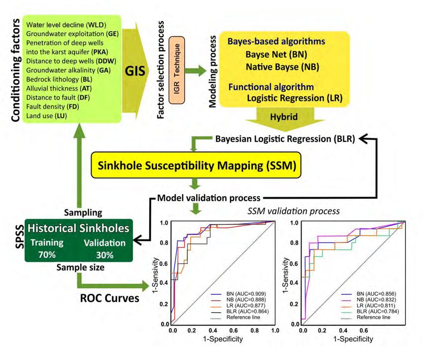
including analytic hierarchy processes (Taheri et al., 2015), frequency ratio (Yilmaz, 2007),
logistic regression (Papadopoulou-Vrynioti et al., 2013; Ciotoli et al., 2016), artificial neural
networks (Yilmaz et al., 2013), and conditional probability (Yilmaz et al., 2013). These
methods provide susceptibility assessments that are objective, reproducible and may reach a
high spatial resolution (Chen et al., 2014). Moreover, high prediction rates have been
demonstrated in some regions (Shirzadi et al., 2017b). However, it is highly necessary to
explore new approaches for sinkhole susceptibility mapping and assess comparatively the
performance of different methods, since any increment in the reliability of the predictions
would have a positive impact on the effectiveness of mitigation plans.
Various machine learning algorithms (MLAs) have been recently developed for analyzing
complex environmental problems that entail land degradation such as sinkholes. The main
advantage of the MLAs is their ability to analyze complex relationships among large datasets.
Additionally, the MLAs can deal with spatial patterns of data at various scales (Kanevski et
al., 2004). The application of these new machine learning predictive models has been
explored in different geoscience fields including landsides (Chen et al., 2015; Chen et al.,
2016; Chen et al., 2017a; Hong et al., 2017), groundwater qanat potential (Naghibi et al.,
2017), or land subsidence (Pradhan et al., 2014). However, their application to sinkhole
susceptibility modelling is still very limited. MLAs have a high computational efficiency,
despite the fact that the models produced with these statistical approaches may have limited
prediction capability and utility related to multiple factors such as the quantity and quality of
the data (epistemic uncertainty) and the inherent spatial-temporal patterns of the phenomenon
and controlling factors (aleatory uncertainty) (Bui et al., 2018a; Bui et al., 2018b;
Shafizadeh-Moghadam et al., 2018). Therefore, identifying the algorithm that allows
developing the best-quality susceptibility models is a critical issue to effectively manage risk
and land-degradation problems associated with sinkhole activity. Hence, the main target of
this study is to evaluate and compare the performance of Naïve Bayes (NB), Bayes Net (BN),
Logistic Regression (LR), and Bayesian Logistic Regression (BLR) classifier models for
sinkhole susceptibility mapping in the northern plains of Hamadan province, Iran. To our best
knowledge, these algorithms have not been applied to sinkhole susceptibility mapping before.

                                        STUDY AREA
The study area includes the Kabudar Ahang and the Razan-Qahavand subcatchments (KRQ)
of the Hoz-e-soltan of Qom watershed, in the northern Hamadan Province, western Iran
(Figure 1). It covers an area of 6,532 km2, of which 3,402 km2 (52%) correspond to alluvial

                                      This article is protected by copyright. All rights reserved.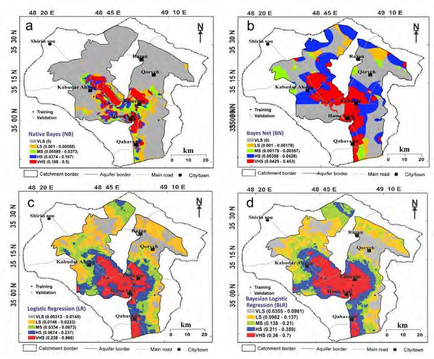
plains and piedmonts. Mean elevation is 1715 m and climate is semi-arid, with 300 mm
average annual precipitation and a mean temperature of 10.5°C (Sabziparvar, 2003).

                                          (Figure 1)

From the geological perspective, the Zagros orogenic belt consists of four main NW-SE
trending structural zones, from NE to SW: Urumieh-Dokhtar Magmatic Assemblage,
Sanandaj-Sirjan, High Zagros Belt, and Zagros Simply Folded Belt (Ghasemi & Talbot,
2006). The study area is situated within the Sanandaj-Sirjan structural zone, in which the
rocks show the highest degree of deformation of this active orogene (Figure 2). The exposed
bedrock consists of a thick Jurassic to Miocene succession including sedimentary and
volcanic rocks affected by folds and thrusts with a dominant NW-SE trend. The Jurassic
succession is made up of recrystallized limestone, shales, sandstones, marls with limestone
intercalations and conglomerates. The Cretaceous units also include limestones, dolostones
and detrital formations. The Eocene Karaj Formation mainly consists of volcanic rocks
(andesite, dacite, green tuff). The so-called “lower red formation” of Oligocene age is made
up of marls and some sandstones and limestones. The main aquifer is the Oligo-Miocene-age
Qom Formation, which is dominated by limestone as well as volcanic rocks (andesite, tuff,
basalt). This karstified limestone is best exposed around Hamakasi village and the Mount
Qoli Abad. The Miocene “upper red formation” is dominantly a detrital unit. The area also
includes sparse outcrops of late Pliocene and probably Pleistocene lava flows that record
recent volcanic activity in the area. Sinkholes in Hamedan area mainly occur in Quaternary
alluvial deposits underlain by the karstified Qom limestone (Heidari et al., 2011; Taheri et
al., 2015). Interestingly, according to borehole and geophysical data, the Quaternary alluvium
in areas affected by recent sinkhole development reaches as much as 150 m in thickness. The
alluvium shows an overall thickness increase towards the central parts of the synclinal basins,
indicative of syntectonic deposition. Borehole data show that the alluvial cover is dominated
by cohesive fine-grained facies, although they grade into coarser deposits (proximal facies)
towards the mountain ranges.
Previous investigations demonstrate that the recent occurrence of numerous sinkholes in the
area is related to groundwater over-exploitation and the associated water table decline (e.g.,
Khanlari et al., 2012). This anthropogenic change in the local hydrological conditions has
favored the internal erosion of cover deposits into significant pre-existing cavities. This
process results in the progressive upward stopping of voids through the thick and cohesive

                                     This article is protected by copyright. All rights reserved.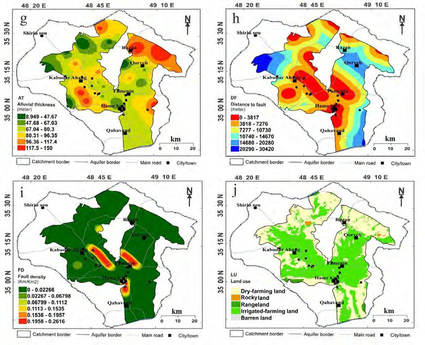
overburden and the development of sudden cover-collapse sinkholes, which is the main
sinkhole type in the area. Some authors also propose that limestone karstification in the
groundwater discharge areas is fostered by renewed aggressiveness due to the incorporation
of deep magmatic fluids along fractures into the flow system. This is supported by the
presence of CO2-rich springs that emerge from the Qom Formation in the vicinity of
Hamakasi village. About 80% of the public-production wells in the area are located in
alluvial deposits, and only 20% penetrate into the karst aquifer. The water balance for the
KRQ alluvial aquifer indicates that around 95% of the recharge is related to irrigation. These
are critical factors that govern groundwater level fluctuations over seasonal and long-term
scales.

                                         (Figure 2)

                                  DATA AND METHODS
Data acquisition
Sinkhole inventory map (SIM)
The SIM was constructed following two steps: (1) field-based sinkhole identification and
recording of their locations, typology, chronology and morphometric parameters, such as
major axial length (D) and depth, and (2) production of a georeferenced sinkhole map. The
inventory includes 47 sinkholes occurred over a period of 22 years (1988-2010) reported by
Taheri et al. (2015). Sinkholes were categorized as cover-collapse sinkholes (86%) and
solution sinkholes (14%) (Karimi & Taheri, 2010).
The major axial length ranges from 1.5 m to 100 m, with an average value of 14.4 m and a
standard deviation of 16.7 m. Average depth is 6.2 m and sinkholes tend to be subcircular,
although reach a maximum elongation ratio (major axial length/minor axial length) of 6.
Maximum estimated volume is greater than 20,000 m3 and around 40% of the sinkholes
exceed 1000 m3 in volume (Taheri et al., 2015). Size and frequency relationships of the
sinkholes using the available chronological data indicate maximum recurrence intervals of
1.2, 2.1 and 4.2 years for sinkholes with lengths of 10, 20 and 30 m, respectively (Taheri et
al., 2015). For the development of susceptibility models, the 47 sinkholes were randomly
divided into training (32 sinkholes) and validation (15 sinkholes) datasets. Furthermore, the
same number of grid cells without sinkholes were randomly selected and partitioned into
training and validation datasets. Table 1 shows the relevant information on the sinkholes
inventoried in the study area.

                                     This article is protected by copyright. All rights reserved.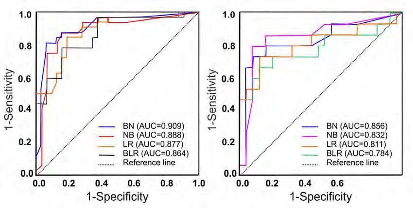
(Table 1)

Field investigation
In this study, initially we gathered information on the location of sinkholes from the
Hamadan Regional Water Authority (HRWA) and each of these sites were checked in the
field. The field surveys in the current study included (i) recording of sinkhole location and
characteristics, (ii) sampling of deposits and bedrock units, and (iii) identification of features
related to some conditioning factors (e.g., rock units, faults) (Taheri et al., 2015).

Sinkhole conditioning factors
The production of sinkhole susceptibility maps was based on the spatial relationships
between the sinkholes of the training dataset and a number of potential conditioning factors.
Thematic maps of ten conditioning factors were produced, which can be divided into three
categories (Figure 3): (1) hydrogeological factors; (2) geological factors; and (3)
anthropogenic factors. Hydrogeological factors include water level decline (WLD),
penetration of deep wells into the karst aquifer (PKA), distance to deep wells (DDW), and
groundwater alkalinity (GA). The geological factors refer to bedrock lithology (BL), alluvial
thickness (AT), distance to faults (DF), and fault density (FD). Groundwater exploitation
(GE) and land use (LU) are the anthropogenic factors considered in this study. Table 2 shows
the factors used for sinkhole susceptibility assessment and data sources. We selected these
factors based on data availability, literature reviews (mainly Taheri et al., 2015), and expert
knowledge.

Water level decline (WLD)
WLD plays an important role in the formation of human-induced sinkholes (Newton, 1984;
Gutiérrez et al., 2016). Data from 65 piezometers covering a 22-year record period (1988-
2010) were used to construct the WLD map by the inverse distance weighted (IDW) method
and differentiating six categories of WLD in meters (Figure 3a).

Groundwater exploitation (GE)
GE accounts for the rate of groundwater pumping from wells in Mm3 per year. It provides
information on the distribution of groundwater withdrawal points and their relative
importance. The data base of the HRWA, including records from 3,850 wells, was utilized for

                                       This article is protected by copyright. All rights reserved.
the preparation of the GE map using the IDW method and discretizing the variable into six
categories (Figure 3b).
Penetration of deep wells into karst aquifer (PKA)
PKA indicates the vertical distance between the top of the bedrock and the bottom of deep
wells. It seems to play a major role in the formation of sinkholes in the study area, especially
in the vicinity of Hamadan Power Plant. The PKA map was produced by the IDW method
and differentiated six categories (Figure 3c).
Distance to deep wells (DDW)
A significant proportion of the reported sinkholes are situated in the proximity of deep wells
mainly drilled by local residents. The incorporation of this factor in the analysis relies on the
hypothesis that the probability of sinkhole occurrence is inversely proportional to the distance
of each point to the nearest deep well. The DDW map was constructed by a buffering method
and discretizing the variable into six classes (Figure 3d).
Groundwater alkalinity (GA)
GA is defined as the total concentration of bicarbonate (HCO3−) and carbonate (CO32−) ions
(Bowman, 1997), reflecting the capability of the water to corrode limestone bedrocks and the
carbonate components of overburden deposits. In general, the higher the alkalinity is, the
lower the aggressiveness of the water will be. The concentration of bicarbonate in the typical
karstic groundwater is around 200 mg/l (Salvati & Sasowsky, 2002), whereas in some parts
of the KRQ it exceeds 1500 mg/l. The GA map was produced by discretizing this continuous
variable into six intervals using the natural break method (Figure 3e).
Bedrock lithology (BL)
BL is a critical factor for the distribution of sinkholes, since a prerequisite for their formation
is the presence of soluble bedrock. Nonetheless, most of the sinkholes occur in areas
extensively covered by Quaternary alluvium, where there is significant uncertainty about the
distribution of the different lithologies that form the rockhead (Heidari et al., 2011). Five
lithotypes have been differentiated in the BL map: schist-shale, marl, limestone, marly
limestone and conglomerate-sandstone (Figure 3f).
This article is protected by copyright. All rights reserved.Alluvial thickness (AT)
A striking characteristic of this area is that sinkholes occur in zones where the limestone
bedrock is covered by a very thick alluvial cover, locally more than 100 m thick (Taheri et
al., 2015). This indicates that deep cavities developed in the bedrock can propagate upwards
by progressive collapse through thick alluvium. The AT map has been generated with the
available borehole data and dividing the variable into six classes by the natural break method
(Figure 3g).
Distance to faults (DF)
The relative spatial distribution of sinkholes and major faults, as well as some patterns like
the elongation and alignment of some sinkholes suggest that the cavities and the associated
subsidence processes may be controlled by tectonic structures (Taheri et al., 2016). The DF
map was produced with the faults depicted in the available 1:100,000 scale geological maps
and categorizing the resulting values into six classes (Figure 3h). The faults used in the
analysis, mostly with reverse displacement, where checked during the field surveys.
Fault density (FD)
Fault density refers to the cumulative length of faults per unit area (Shirzadi et al., 2017a). A
high density of faults in carbonate bedrock may create favorable permeability conditions for
groundwater circulation, the creation of structurally-controlled cavities and the occurrence of
sinkholes. The fault density was calculated using data from the 1:100,000 scale geological
map and was grouped into six classes (Figure 3i).
Land use (LU)
The type of land use may significantly influence some processes involved in sinkhole
development by modifying the natural hydrology and vegetation, notably internal erosion and
cover collapse. The LU map was produced using Operational Land Imager (OLI)-sensor
images captured by Landsat 8 satellite on 10 August 2013 and provided by the National
Geographical Service of Iran. The land-use map differentiates five classes including dry
farming, rocky land, rangeland, irrigated farming and barren land. The land-use classes were
mapped by means of supervised Maximum Likelihood Classification (MLC) using the
ENVI5.1 software (Figure 3j). The resulting normalized difference vegetation index (NDVI)
This article is protected by copyright. All rights reserved.map shows the distribution of different vegetation coverages. This index is between -1 to +1
and was calculated by the following equation (Pradhan et al., 2010):
NDVI=(NIR - VIS)/(NIR + VIS)
(1)
where VIS and NIR are the spectral reflectance acquired in the red band and near-infrared
band, respectively.
(Figure 3)
(Table 2)
Factor selection based on the information gain ratio
Sinkhole occurrence depends on favorable conditions determined by a number of local
factors. Consequently, selecting the factors with higher predictive ability is a critical step in
susceptibility modeling (Pradhan, 2013). In order to increase the prediction capability of the
models and the benefit/effort ratio of the data-gathering and modeling process, the factors
with low or null predictive capability should be removed (Doshi, 2014). These factors can be
identified through the information gain ratio method (IGR) (Quinlan, 1996).
Consider S as a training dataset consisting of n input samples, where n Yi , S is the number
of samples in the training dataset S, belonging to the Yi class (sinkhole, no-sinkhole). The
IGR for a sinkhole conditioning factor such as alluvial thickness (AT) and the training data
(S) is given by:
Entropy (S)-Entropy (S, AT)
IGR S, AT =
SplitEntropy (S, AT)
(2)
2
n(Yi , AT) n(Yi , AT)
Entropy (S) = - log 2
i=1 S S
(3)
m Sj
Entropy (S, AT)= Entropy (S)
j=1 S
(4)
This article is protected by copyright. All rights reserved.m Sj Sj
SplitEntropy ( S , AT ) = - log 2
j=1 S S
(5)
Background on the machine learning algorithms
Naïve Bayes (NB) classifier
NB is a Bayes-based classifier based on conditional independence (CI) (Pham et al., 2017).
In CI, it is assumed that all attributes of examples are independent for maximizing the
posterior probability with given output class for classification issue (Soni et al., 2011). The
main aim of the NB classifier is to compute the prior probabilities of each class using a
discriminant function (Hong et al., 2017). NB has been applied in many scientific fields
because it is very robust to noise and irrelevant attributes and also does not need a big
training dataset for modeling (Tien Bui et al., 2012). For mapping sinkhole susceptibility
using the NB classifier, it was considered x x1 , x2 ,..., x10 as the vector of the ten
conditioning factors and y y1 , y2 as the vector of the dependent variables (sinkhole, no-
sinkhole). The prior probability of NB is obtained using a discriminant function as follows:
10
y NB =argmaxP(yi ) P(x i yi )
i=1
yi =sinkhole,no-sinkhole
(6)
where P(yi ) is prior probability of yi , and P(x i y i ) is the conditional probability obtained
using the following equation:
xi
1
P(x i yi ) e 2 2
2
(7)
where and are the mean and standard deviation of x i , respectively.
Bayes Net (BN) classifier
BN is a Bayes-based graphical classifier with a strong independence assumption. It was
introduced by Friedman et al (1997) to represent the relationships among variables (Song et
al., 2012; Pham et al., 2016b). BN has a power classifier for assessing hazardous events
This article is protected by copyright. All rights reserved.(Liang et al., 2012). BN comprises two components: (1) directed acyclic graph (DAG) of the
nodes in the BN classifiers that are corresponded to conditioning factors, and (2) a
conditional distribution for each node determined by a conditional probability table (CPT).
The CPT for each node can be calculated by Domain Knowledge (DK) using expert and
Parameters Learned (PL) from sample datasets through machine learning or Bayesian
estimation (Liang et al., 2012). The latter was used in this study. If X r represents a node in
the BN classifier, then the joint probability distribution of a sinkhole in relation with a
conditioning factor X can be computed as:
n n
PBN X 1 , X 2 ,..., X n PB ( X 1 ) X
i 1
Xi
i 1
i Xi
(8)
where X = X1 , X 2 ,..., X10 denotes the sinkhole conditioning factors, and
10
PB (X1 Xi ) θX
i=1
i Xi
is a sinkhole joint probability distribution in relation with a
conditioning factor X i , and n is the number of sinkhole conditioning factors.
Logistic Regression (LR)
LR is a multivariate statistical technique, in which the dependent variable should be binary or
dichotomous, such as 0 and 1, or presence and absence of an event, while independent
variables (conditioning factors) can be continuous and categorical (Shirzadi et al., 2012;
Shahabi et al., 2014; Chapi et al., 2017). It is a generalization of a linear model whereby
relationships between the probability of sinkhole occurrence and the ten independent
variables can be quantitatively computed as follows:
ez
PLR
1 ez
(9)
P
Z log it ( P ) Ln ( ) c0 a1 x1 , a2 x2 ,..., an xn
1 P
(10)
where PLR is the probability of sinkhole occurrence, Z is the weighted linear combination of
the independent variables, c0 is the constant or intercept of model, ai (i=0, 1, 2, ..., n) are the
coefficients, and xi i=0, 1, 2 ,..., n are the independent variables (Chen et al., 2017b).
This article is protected by copyright. All rights reserved.Bayesian Logistic Regression (BLR) classifier
The BLR classifier is a combination of the NB classifier and the LR function. This classifier
constructs the relationships between dependent (sinkhole and no-sinkhole) and independent
(ten conditioning factors) variables (Chapi et al., 2017). The Bayesian framework is
constructed in three steps; firstly, the prior probability (PP) is specified for each parameter;
then the likelihood function (LF) is obtained for the dataset, and finally the posterior
probability distribution (PPD) for the parameters is calculated (Avali et al., 2014). Let
x = (x1, x 2 ,..., x n ) be the vector of the sinkhole conditioning factors of the training dataset X,
and y = (y1 , y 2 ) the vector of the classifier dependent variables (sinkhole, no-sinkhole). PPD
for a sample belonging to a specific class can be computed by the logistic function:
1
P(class x1 ,x 2 ,...,x n )= n
(b+w 0 *c+ w i *f(x i ))
(1+exp i=1
(11)
where x i denotes the sinkhole conditioning factors, c is the prior log odds ratio, which is
P (class 0)
obtained using c log ,‘ b ’ is bias, weights w 0 and w i are learned from the
P (class 1)
P (x i class 0)
training dataset, and the i th attribute x i is utilized to obtain f(xi ) using log
P (x i class 1)
(for binary class outcome variables) (Figure 4).
(Figure 4)
Accuracy assessment and comparison
The receiver operating characteristics curve
The receiver operating characteristics curve (ROC) was used for the first time by the United
States army to analyze the detection of radar signals related to Japanese aircrafts during Word
War II (Ingleby, 1967). The aim of the receiver operating characteristic (ROC) method was to
increasing the success rate in the detection of Japanese aircraft from radar signals.
Subsequently, it has been used in psychophysics (Ingleby, 1967), medicine (Zweig &
Campbell, 1993; Pepe, 2003), and meteorology (Kharin & Zwiers, 2003). However, the first
application of the ROC curves in machine learning was carried out by Spackman (1989) for
comparing and evaluating different classification algorithms (Spackman, 1989). The ROC
curve is plotted in a two-dimensional graph with the sensitivity (true positives) in the Y-axis
This article is protected by copyright. All rights reserved.and the specificity (false positives) in the X-axis, respectively. If it is based on the training
dataset, the graph is named success rate curve (SRC) and if it is based on the validation
dataset, it is designated as prediction rate curve (PRC) (Bradley, 1997).
The area under the ROC curve (AUROC) is a measure of the capability of the model to
predict the spatial distribution of events (sinkhole) (Hong et al., 2017). It ranges between 0.5
(null prediction capability) and 1 (perfect model) (Shirzadi et al., 2017a). The AUROC can
be classified into different predictive capability ranks as excellent (0.9-1), very good (0.8-
0.9), good (0.7-0.8), average (0.6-0.7) and poor (0.5-0.6) (Bui et al., 2017). The AUROC can
be expressed as:
AUROC=
TP+ TN
P+N
(12)
where TP is the number of sinkholes that are correctly classified, TN is the number of
incorrectly classified sinkholes, P is the total number of sinkholes, and N is the total number
of no-sinkhole pixels.
Statistical index-based measures
To further validate the performance of the models, some statistical indices including
sensitivity, specificity, accuracy, Kappa index, root mean square error (RMSE), and mean
absolute error (MAE) were used. These measures are obtained using the four possible
consequences: true positive (TP), true negative (TN), false positive (FP), and false negative
(FN). TP and FP are defined as the proportion of sinkhole pixels correctly and incorrectly
classified as sinkhole in the model, respectively. TN and FN are the proportion of the number
of no-sinkhole pixels correctly and incorrectly classified as no-sinkhole, respectively (Pham
et al., 2016a; Shirzadi et al., 2017a). These indices can be formulated as:
TP
Precision =
TP+ FP
(13)
TP
Sensitivity =
TP+ FN
(14)
TN
Specificity =
TN+ FP
(15)
This article is protected by copyright. All rights reserved.TP+ TN
Accuracy =
TP+ TN+ FP+ FN
(16)
PC - Pexp
Kappa index (K) =
1- Pexp
(17)
PC = (TP+ TN) (TP+ TN+ FN+ FP)
(18)
Pexp = TP+ FN TP+ FP + FP+ TN FN+ TN (TP+ TN+ FN+ FP)
(19)
1 n
RMSE =
n
i=1
(X est . - Xobs. ) 2
(20)
1 N
MAE
N
X
i 1
est X obs
(21)
where n is the total number of samples in the training or validation dataset; X est . is the
predicted values in the training or validation datasets; and X obs . is the actual (output) values
from the sinkhole susceptibility models.
Non-parametric statistical assessment
To evaluate significant differences among statistical treatments of two or more machine
learning classifiers without recording their variances, parametric and non-parametric analyses
can be applied. Although parametric statistical tests are utilized when data are normally
distributed with equal variances, the non-parametric Freidman (Friedman, 1937) and
Wilcoxon (Wilcoxon, 1945) tests are free from any statistical assumption. The null
hypothesis is: there is no difference among the performances of sinkhole classifiers at a
significant level of α=0.05 (or 5%). Consequently, based on the probability of a hypothesis
(p-value), the null hypothesis is rejected or accepted if the p-value is true or false,
respectively (Bui et al., 2016). If the p-value in the Freidman test is true in the models, the
results of comparison among two or more models are not reliable. Hence, the Wilcoxon test
is conducted to assess systematic pairwise differences among the sinkhole models using p-
value and z-value. Accordingly, the performance of the sinkhole susceptibility classifiers is
This article is protected by copyright. All rights reserved.significantly different (rejecting the null hypothesis) when the p-value is less than 0.05 and
the z-value exceeds the critical values of z (−1.96 and +1.96) (Bui et al., 2016).
RESULTS AND DISCUSSION
Sinkhole conditioning factor analysis
The prediction capability of the 10 sinkhole conditioning factors was evaluated using the IGR
method in a 10-fold cross-validation on the training dataset (Table 3). The higher the IGR is,
the higher the capability of the factor to predict the spatial distribution of new sinkholes will
be. Results showed that bedrock lithology has the highest impact on sinkhole occurrence
(IGR=0.626), followed by groundwater alkalinity (IGR=0.37), fault density (IGR=0.3),
distance to faults (IGR=0.28), penetration of deep wells into the karst aquifer (IGR=0.205),
water level decline (IGR=0.203), groundwater exploitation (IGR=0.119), and distance to
deep wells (IGR=0.101). IGR revealed that alluvial thickness and land-use, with IGR=0, have
negligible predictive utility. Consequently, these conditioning factors were disregarded for
the susceptibility modeling process. The obtained results are in agreement with Taheri et al.
(2015), who reported that bedrock lithology reached the highest weight in comparison to
other independent variables, using the analytical hierarchy process (AHP) method. Taheri et
al. (2015) also indicated that the distance to deep wells (DDW) has the lowest AHP weight
and has a limited utility for sinkhole modeling.
A critical and particularly challenging task of this work was the production of the data layer
corresponding the bedrock lithology, since sinkholes mainly occur in areas where the bedrock
is concealed by thick alluvium. The boundaries between the different lithological units in the
areas covered by Quaternary deposits were delineated by interpolation, considering the
contacts of the geological maps and the tectonic structures. Moreover, the distribution of
sinkholes in the study area showed that they tend to form clusters and alignments, suggesting
that faults may play a significant spatial control, as previously suggested by Taheri et al.
(2015).
Initially, alluvial thickness and land-use were intuitively considered to be important factors
for the development of the models. However, the computed IGR values revealed that these
factors are not useful for modeling sinkhole susceptibility. It should be noted that these
results are site-specific and may not be applicable in other regions.
(Table 3)
This article is protected by copyright. All rights reserved.Sinkhole susceptibility mapping
After applying the BN, NB, LR and BLR statistical approaches, sinkhole susceptibility
indices (SSIs) were estimated for each pixel in the different models. The SSIs are computed
according to the probability distribution function (PDF) of each approach. For example, in
the BN and NB methods, the PDFs are probability functions, whereas logistic functions are
applied to calculate the SSIs indices in the LR and BLR approaches.
In order to facilitate the visualization of the susceptibility models, the indices were classified
into five susceptibility classes by the natural break method: very low (VLS), low (LS),
moderate (MS), high (HS), very high (VHS). Finally, four susceptibility maps were
developed by the different statistical approaches (Figure 5). These maps consistently indicate
that the central and southwestern parts of the study area, associated with major cartographic
faults, significant water level decline and penetration of deep wells into the karst aquifer have
the highest susceptibility to sinkhole occurrence.
(Figure 5)
Model results and analysis
Once the best conditioning factors and the parameters of the four different models were
determined, their performances were evaluated using both the training (Table 4) and
validation datasets (Table 3).
(Table 4)
According to the training dataset, the BN model has the best performance (goodness of fit)
measured by RMSE, MAE and AUROC, and the NB model shows the best results in terms of
sensitivity, specificity, accuracy, and Kappa indexes. According to the sensitivity criterion,
the NB model (0.938) shows the best quality, with 93.8% of the sinkhole pixels correctly
classified in the sinkhole classes, followed by BN (0.935), BLR (0.903) and LR (0.844). The
NB model also has the highest specificity (0.938), with 93.8% of the no-sinkhole pixels
correctly classified in the no-sinkhole class. The highest accuracy was achieved by the NB
model (0.938), indicating that the probability of correctly classified pixels is 93.8%, followed
by the BN (0.922), BLR (0.891) and LR models (0.844).
The RMSE and MAE computed with the training dataset shows that the BN model has the
highest fit (0.097 and 0.234), followed by the NB (0.107 and 0.271), BLR (0.109 and 0.3)
and LR models (0.226 and 0.336). The NB model has the highest Kappa index (0.875)
This article is protected by copyright. All rights reserved.calculated with the training dataset, indicating an almost perfect agreement between
estimation and observation, followed by the BN (0.843), BLR (0.781), and LR models
(0.681).
The ROC curves produced with the training dataset showed that the BN model has the
highest AUROC (0.977), followed by the NB (0.954), LR (0.914) and BLR models (0.891).
The prediction capability of the four models was evaluated using the validation dataset (Table
5). The four models showed excellent or very good prediction ability with the highest
AUROC for the BN model (0.976), followed by the NB (0.899), BLR (0.867) and LR models
(0.809). The Kappa index varies from 0.6 to 0.733 proving that all the models had almost
perfect agreement with the validation dataset. The highest sensitivity corresponds to the NB
(0.789), BN (0.789), and BLR models (0.789), indicating that 78.9% of the sinkhole pixels
were correctly classified. The BN, NB and BLR models has the highest specificity index
(1.0), with 100% of the no-sinkhole pixels correctly classified, followed by the LR model
(0.909). The BN, NB and BLR models yield the highest accuracy (0.867), followed by the
LR model (0.8). The BN model has the lowest RMSE and MAE (0.148 and 0.339), followed
by the NB (0.151 and 0.362), BLR (0.153 and 0.365) and LR models (0.264 and 0.384).
Overall, the results indicate that the Bayes Net classifier (BN) approach allows generating a
higher quality susceptibility model than the other statistical methods (NB, BLR and LR). The
BN considers the uncertainty interdependence among conditioning factors and provides a
semantic mode to check the missing data, decreasing noise and preventing over-fitting
problems (Liang et al., 2012; Song et al., 2012). The obtained results are in agreement with
Pham et al. (2016b), who compared five machine learning methods, namely Support Vector
Machines (SVM), Logistic Regression (LR), Fisher's Linear Discriminant Analysis (FLDA),
Bayesian Network (BN), and Naïve Bayes (NB) for the spatial prediction of landslides,
concluding that the BN model outperformed the NB model.
(Table 5)
Model validation and comparison
The validity of the four susceptibility maps was quantitatively evaluated by the AUROC
(Figure 6). The area under the success rate curve reaches the highest value for the BN model
(0.909), followed by NB (0.888), LR (0.877) and BLR models (0.864) (Figure 6a). The
highest area under the prediction rate curve was also achieved by BN (0.856), closely
This article is protected by copyright. All rights reserved.followed by NB (0.832), LR (0.811) and BLR (0.784). These values suggest that the BN
model has the highest prediction capability.
(Figure 6)
Results indicated that all the models yield reliable predictions (Tables 5 and 6, and Figure 6).
However, in order to determine whether they show statistically significant differences, the
Freidman and Wilcoxon tests were applied at the 5% significant level (Table 6). Results
indicate that since P-value is 0.000 (lithology; and (2) the factors with negligible statistical significance for sinkhole prediction
(i.e., alluvial thickness and land use). The latter were disregarded in the susceptibility
modeling process since they do not contribute to increase the prediction capability of the
models. This step, which is rarely performed in susceptibility modeling, has several
advantages, including: (1) the identification of the main factors that control the development
of sinkholes, providing useful clues for hazard and risk mitigation, (2) contributes to reduce
the effort/benefit ratio by disregarding particular factors in the data-collection and modeling
process, and (3) may allow producing susceptibility models with higher prediction capability
using a more limited amount of data.
The quantitative and independent evaluation of the susceptibility models developed with the
different machine learning algorithms reveals that Bayes-based models (BN, NB, and BLR)
provide more reliable predictions than statistical model (LR) measured by the AUROC. This
is probably related to the fact that Bayes-based models are more adequate for analyzing
complex phenomena governed by largely hidden factors such as sinkholes. The BN model
produced the most reliable sinkhole susceptibility map.
The results obtained in the Hamadan region offer promising prospects in the field of sinkhole
modeling and risk mitigation. Our findings can be applied by watershed managers,
stakeholders, and land policy makers for managing and mitigating land degradation caused
by sinkholes. However, additional work should be performed in order to assess wether these
findings can be generalized and to improve the quality and usefulness of the predictions. It
would be desirable to apply this methodology in other regions with different geological
conditions and where sinkholes are controlled by other factors. It would be also advisable to
assess the potential impact of improving the accuracy of the factors (e.g. spatial resolution)
on the quality of the models. Moreover, transforming susceptibility models into hazard
models that quantitatively estimate the probability of occurrence of new sinkholes in each
portion of the territory would significantly increase the applicability of the models.
Acknowledgment:
We express our thanks to the Editor-in-Chief of the Land Degradation & Development
journal and four anonymous reviewers for their insightful comments and corrections. The
work carried out by Francisco Gutiérrez is supported by project CGL2017-85045-P (Spanish
Government).
This article is protected by copyright. All rights reserved.References
Avali VR, Cooper GF, Gopalakrishnan V. (2014). Application of Bayesian Logistic Regression to
Mining Biomedical Data. Journal of the American Medical Informatics Association 21, 952-
968. DOI: 10.1136/amiajnl-2014-003170
Bowman RS. (1997). Aqueous environmental geochemistry. Eos, Transactions American
Geophysical Union, 78, 586-586. DOI: 10.1029/97eo00355
Bradley AP. (1997). The use of the area under the ROC curve in the evaluation of machine learning
algorithms. Pattern recognition, 30, 1145-1159. DOI: 10.1016/s0031-3203(96)00142-2
Bui DT, Khosravi K, Li S, Shahabi H, Panahi M, Singh V, Chapi K, Shirzadi A, Panahi S, Chen W.
(2018a). New hybrids of Anfis with several optimization algorithms for flood susceptibility
modeling. Water, 10, 1210-1231. DOI: 10.3390/w10091210
Bui DT, Nguyen QP, Hoang N-D, Klempe H. (2017). A novel fuzzy K-nearest neighbor inference
model with differential evolution for spatial prediction of rainfall-induced shallow landslides in
a tropical hilly area using GIS. Landslides, 14, 1-17. DOI: 10.1007/s10346-016-0708-4
Bui DT, Panahi M, Shahabi H, Singh VP, Shirzadi A, Chapi K, Khosravi K, Chen W, Panahi S, Li S.
(2018b). Novel hybrid evolutionary algorithms for spatial prediction of floods. Scientific
Reports, 8, 15364-1546. DOI: 10.1038/s41598-018-33755-7
Bui DT, Tuan TA, Klempe H, Pradhan B, Revhaug I. (2016). Spatial prediction models for shallow
landslide hazards: a comparative assessment of the efficacy of support vector machines,
artificial neural networks, kernel logistic regression, and logistic model tree. Landslides, 13,
361-378. DOI: 10.1007/s10346-015-0557-6
Chapi K, Singh VP, Shirzadi A, Shahabi H, Bui DT, Pham BT, Khosravi K. (2017). A novel hybrid
artificial intelligence approach for flood susceptibility assessment. Environmental Modelling &
Software, 95, 229-245. DOI: 10.1016/j.envsoft.2017.06.012
Chen T, Niu R, Du B, Wang Y. (2015). Landslide spatial susceptibility mapping by using GIS and
remote sensing techniques: a case study in Zigui County, the Three Georges reservoir, China.
Environmental Earth Sciences, 73, 5571-5583. DOI: 10.1007/s12665-014-3811-7
Chen T, Niu R, Jia X. (2016). A comparison of information value and logistic regression models in
landslide susceptibility mapping by using GIS. Environmental Earth Sciences, 75, 867-876.
DOI: 10.1007/s12665-016-5317-y
Chen T, Trinder JC, Niu R. (2017a). Object-oriented landslide mapping using ZY-3 satellite imagery,
random forest and mathematical morphology, for the Three-Gorges Reservoir, China. Remote
Sensing, 9, 333-349. DOI: 10.3390/rs9040333
Chen W, Li X, He H, Wang L. (2017). A review of fine-scale land use and land cover classification in
open-pit mining areas by remote sensing techniques. Remote Sensing, 10, 1-19. DOI:
10.3390/rs10010015
Chen W, Li X, Wang Y, Chen G, Liu S. (2014). Forested landslide detection using LiDAR data and
the random forest algorithm: A case study of the Three Gorges, China. Remote Sensing of
Environment, 152, 291-301. DOI: 10.1016/j.rse.2014.07.004
Chen W, Pourghasemi HR, Zhao Z. (2017b). A GIS-based comparative study of Dempster-Shafer,
logistic regression and artificial neural network models for landslide susceptibility mapping.
Geocarto International, 32, 367-385. DOI: 10.1080/10106049.2016.1140824
Ciotoli G, Di Loreto E, Finoia M, Liperi L, Meloni F, Nisio S, Sericola A. (2016). Sinkhole
susceptibility, Lazio Region, central Italy. Journal of Maps, 12, 287-294. DOI:
10.1080/17445647.2015.1014939
Doshi M. (2014). Correlation Based Feature Selection (Cfs) Technique To Predict Student
Perfromance. International Journal of Computer Networks & Communications, 6, 197-206.
DOI: 10.5121/ijcnc.2014.6315
Filippi M, Bosák P. (2013). Proceedings of the16th International congress of speleology, Czech
Speleological Society. Brno, 21-28 July 2013. 2, 453.
Ford D, Williams PD. (2013). Karst hydrogeology and geomorphology. New York: John Wiley &
Sons Ltd.
Friedman M. (1937). The use of ranks to avoid the assumption of normality implicit in the analysis of
variance. Journal of the American Statistical Association, 32, 675-701. DOI: 10.2307/2279169
This article is protected by copyright. All rights reserved.Friedman N, Geiger D, Goldszmidt M. (1997). Bayesian network classifiers. Machine Learning, 29,
131-163. DOI: 10.7/1-412-43-7
Galve J, Gutiérrez F, Lucha P, Bonachea J, Remondo J, Cendrero A, Gutiérrez M, Gimeno M, Pardo
G, Sánchez J. (2009). Sinkholes in the salt-bearing evaporite karst of the Ebro River valley
upstream of Zaragoza City (NE Spain): Geomorphological mapping and analysis as a basis for
risk management. Geomorphology, 108, 145-158. DOI: 10.1016/j.geomorph.2008.12.018
Ghasemi A, Talbot CJ. (2006). A new tectonic scenario for the Sanandaj–Sirjan Zone (Iran). Journal
of Asian Earth Sciences, 26, 683-693. DOI: 10.1016/j.jseaes.2005.01.003
Gunn J. (2004). Encyclopedia of caves and karst science. New York: Taylor & Francis.
Gutiérrez F, Fabregat I, Roqué C, Carbonel D, Guerrero J, García-Hermoso F, Zarroca M, Linares R.
(2016). Sinkholes and caves related to evaporite dissolution in a stratigraphically and
structurally complex setting, Fluvia Valley, eastern Spanish Pyrenees. Geological,
geomorphological and environmental implications. Geomorphology, 267, 76-97. DOI:
10.1016/j.geomorph.2016.05.018
Gutiérrez F, Parise M, De Waele J, Jourde H. (2014). A review on natural and human-induced
geohazards and impacts in karst. Earth-Science Reviews, 138, 61-88. DOI:
10.1016/j.earscirev.2014.08.002
Heidari M, Khanlari G, Beydokhti AT, Momeni A. (2011). The formation of cover collapse sinkholes
in North of Hamedan, Iran. Geomorphology, 132, 76-86. DOI:
10.1016/j.geomorph.2011.04.025
Hong H, Liu J, Zhu A-X, Shahabi H, Pham BT, Chen W, Pradhan B, Bui DT. (2017). A novel hybrid
integration model using support vector machines and random subspace for weather-triggered
landslide susceptibility assessment in the Wuning area (China). Environmental Earth Sciences,
76, 652-663. DOI: 10.1007/s12665-017-6981-2
Hyland SE. (2005). Analysis of sinkhole susceptibility and karst distribution in the northern
Shenandoah Valley, Virginia: implications for low impact development (LID) site suitability
models. Virginia Polytechnic Institute and State University.
Ingleby J. (1967). Book Review: Signal detection theory and psychophysics. by DM Green and JA
Swets. New York: John Wiley & Sons Ltd, 1966. Cloth. 104s. Journal of Sound Vibration, 5,
519-521. DOI: 10.1016/0022-460X(67)90197-6
Jafari R, Bakhshandehmehr L. (2016). Quantitative mapping and assessment of environmentally
sensitive areas to desertification in central Iran. Land Degradation & Development, 27, 108-
119. DOI: 10.1002/ldr.2227
Kanevski M, Parkin R, Pozdnukhov A, Timonin V, Maignan M, Demyanov V, Canu S. (2004).
Environmental data mining and modeling based on machine learning algorithms and
geostatistics. Environmental Modelling & Software, 19, 845-855. DOI:
10.1016/j.envsoft.2003.03.004
Karimi H, Taheri K. (2010). Hazards and mechanism of sinkholes on Kabudar Ahang and Famenin
plains of Hamadan, Iran. Natural Hazards, 55, 481-499. DOI: 10.1007/s11069-010-9541-6
Khanlari G, Heidari M, Momeni AA, Ahmadi M, Beydokhti AT. (2012). The effect of groundwater
overexploitation on land subsidence and sinkhole occurrences, western Iran. Quarterly Journal
of Engineering Geology and Hydrogeology, 45, 447-456. DOI: 10.1144/qjegh2010-069
Kharin VV, Zwiers FW. (2003). On the ROC score of probability forecasts. Journal of Climate, 16,
4145-4150. DOI: 10.1175/1520-0442(2003)012.0.co;2
Liang W-j, Zhuang D-f, Jiang D, Pan J-j, Ren H-y. (2012). Assessment of debris flow hazards using a
Bayesian Network. Geomorphology, 171, 94-100. DOI: 10.1016/j.geomorph.2012.05.008
Minaei M, Shafizadeh‐Moghadam H, Tayyebi A. (2018). Spatiotemporal nexus between the pattern
of land degradation and land cover dynamics in Iran. Land Degradation & Development, 29,
2854-2863. DOI: 10.1002/ldr.3007
Naghibi SA, Pourghasemi HR, Abbaspour K. (2017). A comparison between ten advanced and soft
computing models for groundwater qanat potential assessment in Iran using R and GIS.
Theoretical and Applied Climatology, 131, 967 to 984. DOI: 10.1007/s00704-016-2022-4
Newton J. (1984). Natural and induced sinkhole development in the eastern United States. In
Proceedings of the Third International Symposium on Land Subsidence, International
Association of Hydrological Sciences, Wallingford, UK; 549-564.
This article is protected by copyright. All rights reserved.Papadopoulou-Vrynioti K, Bathrellos GD, Skilodimou HD, Kaviris G, Makropoulos K. (2013). Karst
collapse susceptibility mapping considering peak ground acceleration in a rapidly growing
urban area. Engineering Geology, 158. DOI: 10.1016/j.enggeo.2013.02.009 77-88
Parise M. (2013). Recognition of instability features in artificial cavities. In: Filippi M, Bosak P (eds)
Proceedings of the 16th International Congress of Speleology; Brno, 21–28 July 2013, 2, 224–
229.
Pepe MS. (2003). The statistical evaluation of medical tests for classification and prediction. Oxford
Statistical Science Series, UK
Pham BT, Bui D, Prakash I, Dholakia M. (2016a). Evaluation of predictive ability of support vector
machines and naive Bayes trees methods for spatial prediction of landslides in Uttarakhand
state (India) using GIS. Journal of Geomatics, 10, 71-79. DOI: oi.org/10.18165/ig/v6i1.08
Pham BT, Bui DT, Pourghasemi HR, Indra P, Dholakia M. (2017). Landslide susceptibility
assesssment in the Uttarakhand area (India) using GIS: a comparison study of prediction
capability of naïve bayes, multilayer perceptron neural networks, and functional trees methods.
Theoretical and Applied Climatology, 128, 255-273. DOI: 10.1007/s00704-015-1702-9
Pham BT, Pradhan B, Bui DT, Prakash I, Dholakia M. (2016b). A comparative study of different
machine learning methods for landslide susceptibility assessment: a case study of Uttarakhand
area (India). Environmental Modelling & Software, 84, 240-250. DOI:
10.1016/j.envsoft.2016.07.005
Pradhan B. (2013). A comparative study on the predictive ability of the decision tree, support vector
machine and neuro-fuzzy models in landslide susceptibility mapping using GIS. Computers &
Geosciences, 51, 350-365. DOI: 10.1016/j.cageo.2012.08.023
Pradhan B, Abokharima MH, Jebur MN, Tehrany MS. (2014). Land subsidence susceptibility
mapping at Kinta Valley (Malaysia) using the evidential belief function model in GIS. Natural
Hazards, 73, 1019-1042. DOI: 10.1007/s11069-014-1128-1
Pradhan B, Oh H-J, Buchroithner M. (2010). Weights-of-evidence model applied to landslide
susceptibility mapping in a tropical hilly area. Geomatics, Natural Hazards and Risk, 1, 199-
223. DOI.org/10.1080/19475705.2010.498151
Quinlan JR. (1996). Bagging, boosting, and C4. 5. In AAAI/IAAI, 1; 725-730.
Sabziparvar A. (2003). The analysis of aridity and meteorological drought indices in west of Iran. Bu-
Ali Sina University, Iran.
Salvati R, Sasowsky ID. (2002). Development of collapse sinkholes in areas of groundwater
discharge. Journal of Hydrology, 264, 1-11. DOI: 10.1016/s0022-1694(02)00062-8
Shafizadeh-Moghadam H, Valavi R, Shahabi H, Chapi K, Shirzadi A. (2018). Novel forecasting
approaches using combination of machine learning and statistical models for flood
susceptibility mapping. Journal of Environmental Management, 217, 1-11. DOI:
10.1016/j.jenvman.2018.03.089
Shahabi H, Khezri S, Ahmad BB, Hashim M. (2014). Landslide susceptibility mapping at central Zab
basin, Iran: a comparison between analytical hierarchy process, frequency ratio and logistic
regression models. Catena, 115, 55-70. DOI: 10.1016/j.catena.2013.11.014
Shirzadi A, Bui DT, Pham BT, Solaimani K, Chapi K, Kavian A, Shahabi H, Revhaug I. (2017a).
Shallow landslide susceptibility assessment using a novel hybrid intelligence approach.
Environmental Earth Sciences, 76, 60-79. DOI: 10.1007/s12665-016-6374-y
Shirzadi A, Saro L, Joo OH, Chapi K. (2012). A GIS-based logistic regression model in rock-fall
susceptibility mapping along a mountainous road: Salavat Abad case study, Kurdistan, Iran.
Natural Hazards, 64, 1639-1656. DOI: 10.1007/s11069-012-0321-3
Shirzadi A, Shahabi H, Chapi K, Bui DT, Pham BT, Shahedi K, Ahmad BB. (2017b). A comparative
study between popular statistical and machine learning methods for simulating volume of
landslides. Catena, 157, 213-226. DOI: 10.1016/j.catena.2017.05.016
Song Y, Gong J, Gao S, Wang D, Cui T, Li Y, Wei B. (2012). Susceptibility assessment of
earthquake-induced landslides using Bayesian network: a case study in Beichuan, China.
Computers & Geosciences, 42, 189-199. DOI: 10.1016/j.cageo.2011.09.011
Soni J, Ansari U, Sharma D, Soni S. (2011). Predictive data mining for medical diagnosis: An
overview of heart disease prediction. International Journal of Computer Applications, 17, 43-
48. DOI: 10.5120/2237-2860
This article is protected by copyright. All rights reserved.Spackman KA. (1989). Signal detection theory: Valuable tools for evaluating inductive learning. In
Proceedings of the sixth international workshop on Machine learning. Cornell University,
Ithaca, New York (USA); 160-163. DOI: 10.1016/b978-1-55860-036-2.50047-3
Symeonakis E, Karathanasis N, Koukoulas S, Panagopoulos G. (2016). Monitoring sensitivity to land
degradation and desertification with the environmentally sensitive area index: The case of
Lesvos Island. Land Degradation & Development, 27, 1562-1573. DOI: 10.1002/ldr.2285
Taheri K, Gutiérrez F, Mohseni H, Raeisi E, Taheri M. (2015). Sinkhole susceptibility mapping using
the analytical hierarchy process (AHP) and magnitude–frequency relationships: a case study in
Hamadan Province, Iran. Geomorphology, 234, 64-79. DOI: 10.1016/j.geomorph.2015.01.005
Taheri K, Taheri M, Parise M. (2016). Impact of intensive groundwater exploitation on an
unprotected covered karst aquifer: a case study in Kermanshah Province, western Iran.
Environmental Earth Sciences, 75, 1221. DOI: 10.1007/s12665-016-5995-5
Tien Bui D, Pradhan B, Lofman O, Revhaug I. (2012). Landslide susceptibility assessment in vietnam
using support vector machines, decision tree, and naive bayes models. Mathematical Problems
in Engineering, 2012, 1-26. DOI: 10.1155/2012/974638
Tien Bui D, Shahabi H, Shirzadi A, Chapi K, Pradhan B, Chen W, Khosravi K, Panahi M, Bin Ahmad
B, Saro L. (2018). Land subsidence susceptibility mapping in South Korea using machine
learning algorithms. Sensors, 18, 2464. DOI: 10.3390/s18082464
Vattano M, Parise M, Lollino P, Bonamini M, Maggio D, Madonia G. (2013). Examples of
anthropogenic sinkholes in Sicily and comparison with similar phenomena in southern Italy. In
Proceedings of the 13th Multidisciplinary Conference on Sinkholes and the Engineering and
Environmental Impacts of Karst. National Cave and Karst Research Institute: Carlsbad (New
Mexico, USA): NCKRI Symposium 2; 263-271.
Wilcoxon F. (1945). Individual comparisons by ranking methods. Biometrics Bulletin, 1, 80-83. DOI:
10.2307/3001968
Yilmaz I. (2007). GIS based susceptibility mapping of karst depression in gypsum: a case study from
Sivas Basin (Turkey). Engineering Geology, 90, 89-103. DOI: 10.1016/j.enggeo.2006.12.004
Yilmaz I, Marschalko M, Bednarik M. (2013). An assessment on the use of bivariate, multivariate and
soft computing techniques for collapse susceptibility in GIS environ. Journal of Earth System
Science, 122, 371-388. DOI: 10.1007/s12040-013-0281-3
Youssef AM, Al-Harbi HM, Gutiérrez F, Zabramwi YA, Bulkhi AB, Zahrani SA, Bahamil AM,
Zahrani AJ, Otaibi ZA, El-Haddad BA. (2016). Natural and human-induced sinkhole hazards in
Saudi Arabia: distribution, investigation, causes and impacts. Hydrogeology Journal, 24, 625-
644. DOI: 10.1007/s10040-015-1336-0
Zweig MH, Campbell G. (1993). Receiver-operating characteristic (ROC) plots: a fundamental
evaluation tool in clinical medicine. Clinical Chemistry, 39, 561-577. DOI: 10.2172/1093414
This article is protected by copyright. All rights reserved.You can also read