Smith-Purcell radiation of a vortex electron
←
→
Page content transcription
If your browser does not render page correctly, please read the page content below
Smith-Purcell radiation of a vortex electron
                                                         A. Pupasov-Maksimov and D. Karlovets
arXiv:2102.00278v1 [quant-ph] 30 Jan 2021

                                                         Universidade Federal de Juiz de Fora, Brasil
                                                         Tomsk State University, Russia
                                                         E-mail: tretiykon@yandex.ru,d.karlovets@gmail.com

                                                         Janyary 2021

                                            Keywords: Vortex electron, orbital angular momentum, Smith-Purcell radiation, non-paraxial effects,
                                            grating, quadrupole moment

                                                         Abstract. A wide variety of emission processes by electron wave packets with an orbital angular
                                                         momentum `~, called the vortex electrons, can be influenced by a nonparaxial contribution due to
                                                         their intrinsic electric quadrupole moment. We study Smith-Purcell radiation from a conducting
                                                         grating generated by a vortex electron, described as a generalized Laguerre-Gaussian packet, which
                                                         has an intrinsic magnetic dipole moment and an electric quadrupole moment. By using a multipole
                                                         expansion of the electromagnetic field of such an electron, we employ a generalized surface-current
                                                         method, applicable for a wide range of parameters. The radiated energy contains contributions from
                                                         the charge, from the magnetic moment, and from the electric quadrupole moment, as well as from
                                                         their interference. The quadrupole contribution grows as the packet spreads while propagating, and
                                                         it is enhanced for large `. In contrast to the linear growth of the radiation intensity from the charge
                                                         with a number of strips N , the quadrupole contribution reveals an N 3 dependence, which puts a limit
                                                         on the maximal grating length for which the radiation losses stay small. We study spectral-angular
                                                         distributions of the Smith-Purcell radiation both analytically and numerically and demonstrate that
                                                         the electron’s vorticity can give rise to detectable effects for non-relativistic and moderately relativistic
                                                         electrons. On a practical side, preparing the incoming electron’s state in a form of a non-Gaussian
                                                         packet with a quadrupole moment – such as the vortex electron, an Airy beam, a Schrödinger cat
                                                         state, and so on – one can achieve quantum enhancement of the radiation power compared to the
                                                         classical linear regime. Such an enhancement would be a hallmark of a previously unexplored quantum
                                                         regime of radiation, in which non-Gaussianity of the packet influences the radiation properties much
                                                         stronger than the quantum recoil.
Smith-Purcell radiation of a vortex electron 2
1. Introduction
It was argued that different radiation processes with the vortex electrons carrying orbital angular
momentum `~ with respect to a propagation axis can be investigated using beams of the electron
microscopes [1, 2]. For instance, Vavilov-Cherenkov radiation and transition radiation are affected
by vortex structure of the electron wave packet [2, 3] and an azimuthal asymmetry of the transition
radiation, if detected, would manifest the magnetic moment contribution to the radiation. Another
radiation process, which we study in the present paper, is the Smith-Purcell (S-P) radiation [4] of the
vortex electrons. Specifically, we investigate how the OAM and the spatial structure of the vortex
wave packet influence the radiation characteristics, such as the spectral-angular distributions of the
radiated energy.
The Smith-Purcell radiation mechanism represents a relatively simple way to generate quasi-
monochromatic radiation from charged (electron) bunches passing near a conducting diffraction
grating and it has been proved to be useful in developing compact free electron lasers [5–8] and
high-resolution sensors for the particle beam diagnostics [9–11]. Besides the fundamental interest to
the properties of radiation generated by non-Gaussian packets (in particular, by the vortex electrons),
there are possible applications in electron microscopy [12] and in acceleration of the vortex electrons
via inverse S-P effect [13]. We consider the simplest possible geometry in which the electron wave
packet moves above an ideally conducting diffraction grating (see Fig. 1), which is made of N
rectangular strips of a width a and with a period d. The radiation spectrum consists of diffraction
lines according to the following dispersion relation:
d 1
λg = − cos Θ , g = 1, 2, 3, . . . , (1)
g β
whose width is Γ ≈ 1/N .
As we demonstrate hereafter, such a radiation mechanism is more sensitive to the shape of the
electron packet than Vavilov-Cherenkov radiation or transition radiation, studied in [2, 3]. A quantum
packet always spreads while propagating; however, this does not affect the radiation properties if the
radiation formation length is shorter than the packet’s Rayleigh length, i.e. the distance where
the packet doubles its size. A non-relativistic or moderately relativistic electron packet can become
significantly wider while moving above a grating with a micrometer or millimeter period, so the Smith-
Purcell radiation represents a good tool for studying these effects as the grating can be longer than
the Rayleigh length. As we have recently argued, the spreading influences the radiation properties
only for wave packets with intrinsic multipole moments [14]‡.
First, in section 2, recalling basic properties of Laguerre-Gaussian wave packets we perform a
qualitative analysis to emphasize physics of possible differences from the standard S-P radiation of
‡ Which is the case for vortex electrons, while spherically symmetric Gaussian packet do not possess intrinsic multipole
momentsSmith-Purcell radiation of a vortex electron 3
Figure (1) Generation of Smith-Purcell radiation by a Laguerre-Gaussian (LG) packet characterized
with a charge e, the magnetic moment µ, and with the electric quadrupole moment Qα,β . Two latter
quantities are non-vanishing due to intrinsic angular momentum of the vortex electron. The number
of the grating strips N cannot be larger than Nmax due to the spreading.
an ordinary electron. We also establish values of the parameters – a size of the wave-packet, the
orbital angular momentum, velocity, etc. – that are compatible with our calculation scheme based
on a multipole expansion.
In section 3 we calculate the spectral-angular distribution of the radiation applying a method
of the generalized surface currents [15], which represents a generalization of the known models put
forward by Brownell, et al. [16] and by Potylitsyn, et al. [17]. Explicit relativistic expressions for the
electromagnetic fields produced by a Laguerre-Gaussian wave packet [18] are presented in section 3.2.
Calculations of the radiation fields in the wave zone in section 3.3 involve standard planar Fourier
integrals with respect to x − z coordinates and time. Integration along z direction is tricky because
of the wave packet spreading and of the increasing quadrupole moment. To guarantee validity of the
multipole expansion when calculating the fields, it is necessary to limit the maximal grating length.
With analytical expressions at hand, we analyze in section 4 corrections to the Smith-Purcell
radiation of the point charge. In section 4.1 we analyze the shape and the position of the spectral
line. Our analytical results suggest, that the spreading of the quantum wave packet does not lead to
a broadening of the spectral line (in a contrast to the case of a classical spreading beam). NumericalSmith-Purcell radiation of a vortex electron 4
studies of the spectral lines reveal not only an absence of the broadening, but even a slight narrowing
of the lines due to the charge-quadrupole interference.
The angular distribution is considered in section 4.2. The contribution from the magnetic
moment results in the azimuthal asymmetry similar to diffraction radiation [2]. In section 4.3 we
demonstrate that the quadrupole contribution is dynamically enchanced along the grating. Such a
coherent effect can be seen in the nonlinear growth of the radiation intensity with the grating length.
At the same time, the maximum of the radiation intensity with respect to the polar angle is shifted
towards smaller angles.
For the currently achieved OAM values of ` ∼ 1000 [19] (see also [20–22]), contributions from
both the magnetic moment and the electric quadrupole moment can be, in principle, detected as
discussed in the Conclusion.
Throughout the paper we use the units with ~ = c = |e| = 1.
2. Vortex electrons and multipole moments
2.1. Laguerre-Gaussian packets and non-paraxial regime
Analogously to optics, there are two main models of the vortex particles – the Bessel beams and
the paraxial Laguerre-Gaussian (LG) packets [1]. There is also a non-paraxial generalization of the
latter, called the generalized LG packet [18],
s 2|`|+3
i2n+` ρ|`| ` 4 `ρ2 hpi2
n! |`|
n
ψ`,n (r, t) = L exp − it + ihpiz + i`φr −
(n + |`|)! π 3/4 (ρ̄(t))|`|+3/2 n (ρ̄(t))2 2m
3 t `((td − it)) 2 2
o
− i 2n + |`| + arctan( ) − ρ + (z − huit) ,
Z 2 td 2td (ρ̄(t))2
p
d3 r |ψ`,n (r, t)|2 = 1, ρ = x2 + y 2 , (2)
which represents an exact non-stationary solution to the Schrödinger equation and whose centroid
propagates along the z axis. The paraxial LG packets and the Bessel beams represent two limiting
cases of this model [23]. Below we consider this packet with n = 0 only. Note that the factor 3/2
in the Gouy phase in (2) comes about because the packet is localized in a 3-dimensional space (cf.
Eq.(61) in [23]).
In what follows, we employ the mean radius of the wave packet ρ̄0 instead of the beam waist σ⊥ ,
p q
σ⊥ = ρ̄0 / |`|, ρ̄(t) = ρ̄0 1 + t2 /t2d .
As explained in [24], depending on the
p experimental conditions one could either fix the beam waist,
and so the mean radius ρ̄0 scales as |`|, or fix the radius itself. In this paper, we follow the latter
approach and treat ρ̄0 as an OAM-independent value. p An approach with the fixed beam waist σ⊥
can easily be recovered when substituting ρ̄0 → σ⊥ |`|.Smith-Purcell radiation of a vortex electron 5
Although non-paraxial effects are nearly always too weak to play any noticeable role, the
difference between this non-paraxial LG packet and the paraxial one becomes crucial for a moderately
relativistic particle with β . 0.9. In this regime, which is the most important one for the current
study, it is only Eq.(2) that yields correct predictions for observables and is compatible with the
general CPT-symmetry [18]. As we argue below, the non-paraxial effects are additionally enhanced
when the packet’s spreading becomes noticeable and the OAM is large.
The packet spreads and its transverse area is doubled during a diffraction time td ,
2
mρ̄20 tc ρ̄0
td = =
tc , (3)
|`| |`| λc
which is large compared to the Compton time scale tc = λc /c ≈ 1.3 × 10⁻²¹ sec., λc ≈ 3.9 × 10⁻¹¹ cm.
When the LG packet moves nearby the grating, the finite spreading time (3) puts an upper limit on
the possible impact parameter h, on the initial mean radius of the packet and on the grating length.
Indeed, both the corresponding solution of the Schrödinger equation and the multipole expansion
have a sense only for as long as ρ̄(t) < h or, alternatively,
s
t h2
< − 1. (4)
td ρ̄20
q 2
Let tmax = td hρ̄2 − 1 be the time during which the packet spreads to the extent that it touches the
0
grating§; then the corresponding number of strips Nmax is
r
β ρ̄0 h ρ̄2
Nmax = βtmax /d = 1 − 02 . (5)
|`| λc d h
The geometry implies that ρ̄0 < h = ρ̄(tmax ) or ρ̄0
h for the long grating. In practice, only small
diffraction orders of the radiation can be considered, so that d ∼ βλ for the emission angles Θ ∼ 90◦ .
So an upper limit for the number of strips in this case is
1 ρ̄0 h
Nmax . . (6)
|`| λc λ
If this condition is violated, the multipole expansion is no longer applicable. A rough estimate of the
maximal number of strips for h ≈ hef f ∼ 0.1λ, β ≈ 0.5, ρ̄0 ∼ 1 nm yields
103
Nmax . . (7)
|`|
So if Nmax
1, then |`| < 103 .
The Laguerre-Gaussian electron packet carries, in addition to the charge, higher multipole
moments [25, 26]. In particular, at the distances larger than the mean radius of the vortex packet,
r & ρ̄(t), (8)
§ This results in the so-called grating transition radiation, which we do not study in this paper, although the problem
in which a part of the electron packet touches the grating and another part does not is definitely interesting to explore.Smith-Purcell radiation of a vortex electron 6
it is sufficient to keep a magnetic dipole moment and an electric quadrupole moment [18, 23],
1 2 λ2c
`
µ = ẑ 1− ` 2 , Qαβ (t) = (ρ̄(t))2 diag{1/2, 1/2, −1}. (9)
2m 2 ρ̄0
The magnetic moment includes a non-paraxial correction according to Eq.(45) in [23], which is written
for the case |`|
1. The field of the electron’s quadrupole moment originates from a non-point source
as the quadrupole has a finite width, which is just equal to an rms-radius of the packet.
Note that although an LG packet with ` = 0 has a vanishing quadrupole moment, an OAM-
less packet with a non-vanishing quadrupole momentum can be easily constructed by making this
packet highly asymmetric in shape. Thus our conclusions below can also be applied to an arbitrary
non-symmetric wave packet with a non-vanishing quadrupole moment.
When the spreading is essential – at t & td – the inequality (8) can be violated and the multipole
expansion cannot be used at all. Thus, the conventional (paraxial) regime of emission takes place
only when the spreading is moderate, t . td . Remarkably, the non-paraxial regime of emission
favors moderately large values of the OAM, in contrast to the enhancement of the magnetic moment
contribution for which the OAM should be as large as possible. This is because the quadrupole
moment has a finite radius and so the radiation is generated as if the charge were continuously
distributed along all the coherence length and not confined to a point within this length [14].
2.2. Qualitative analysis and multipole expansion
Single-electron regime with a freely propagating packet is realized for low electron currents – below
the so-called start current, which is typically about 1 mA [27]. The charge, the magnetic dipole
and the electric quadrupole moments (9) induce surface currents on the grating. These currents, in
their turn, generate electric and magnetic fields Ee , Eµ , EQ , etc. The total radiation intensity dW
includes the multipole radiation intensities as well their mutual interference, which serve as small
corrections to the classical radiation from the point charge dWee :
dW
≡ dW = dWee +dWeµ +(dWeQ +dWµµ )+(dWµQ +dWeO )+(dWQQ +dWe16p +dWµO )+. . . (10)
dωdΩ
In this paper, we adhere to such a perturbative regime and formally order perturbative corrections
following the order of the multipole expansion. The leading order (LO) correction dWeµ is given
by the charge-magnetic-moment radiation. The next-to-leading (NLO) order corrections include
the charge-electric-quadrupole radiation dWeQ and the radiation of the magnetic moment dWµµ .
Moreover, in the overwhelming majority of practical cases it is sufficient to calculate the charge
contribution and the interference terms
dW = dWee + dWeµ + dWeQ (11)
only, while dWµµ , dWµQ , and the higher-order corrections can be safely neglected. We emphasize
that it does not mean that there are simple inequalities like dWee
dWeµ
dWeQ
dWµQ ... forSmith-Purcell radiation of a vortex electron 7
all the angles and frequencies. For instance, in the plane perpendicular to the grating, Φ = π/2,
the term dWeµ vanishes while dWeQ does not (see below). This makes the region of angles Φ ≈ π/2
preferable for detection of the non-paraxial quadrupole effects.
An approach in which the particle trajectory is given holds valid when the quantum recoil ηq is
small compared to the interference corrections dWeµ and dWeQ ,
ω dWeµ ω dWeQ
ηq :=
,
, (12)
ε dWee ε dWee
and the energy losses stay small compared to the electron’s energy. We emphasize that the multipole
contributions in Eq.(10) also have a quantum origin as they are due to non-Gaussianity of the wave
packet or, in other words, due to its non-constant phase. So the series (10) is not quasi-classical. On
a more fundamental level, there are two types of quantum corrections to the classical radiation of
charge [28–32]:
• Those due to recoil,
• Those due to finite coherence length of the emitting particle.
While the quasi-classical methods like an operator method [32] and the eikonal method [31] neglect
the latter effects from the very beginning and take into account the recoil only, here we demonstrate
that there is an opposite non-paraxial regime of emission.
Let us study dimensionless parameters that define multipole corrections to the classical emission
of a charge. The magnetic moment contribution (see Eqs. (68),(69)) is proportional to the following
ratio:
dWeµ λc
∼ ηµ := ` , (13)
dWee λ
which is of the order of ` · 10−7 for λ ∼ 1 µm, and ` · 10−10 for λ ∼ 1 mm. It is well known that a
spin-induced magnetic moment contribution – the so-called "spin light" [33] – and the recoil effects
are of the same order of magnitude; thus we neglect both of them in our approach. However, for the
vortex electron the magnetic moment contribution (13) is ` times enhanced, which legitimates the
calculations of dWeµ via the multipole expansion [2]. Indeed, for the electrons with β ≈ 0.4 − 0.8
and the kinetic energy of εc ∼ 50 − 300 keV, the small parameter governing the quantum recoil is
ω 1 λc
ηq = ∼ ≡ , (14)
ε mλ λ
and ηq
ηµ yields
|`|
1,
while the condition ηµ2
ηq puts an upper limit on the OAM value,
r
λ
|`| . `max := ∼ ηq−1/2 ∼ 103 − 105 , λ ∼ 1 µm − 1 mm, (15)
λc
and so the contribution dWµµ stays small.Smith-Purcell radiation of a vortex electron 8
As shown in section 3.1, one can distinguish three different corrections from the charge-
quadrupole interference: dWeQ0 , dWeQ1 , and dWeQ2 . Their relative contributions are:
dWeQ0 ρ̄2
∼ ηQ0 := 20 − quasi-classical quadrupole contribution, (16)
dWee heff
2
dWeQ1 2 λc
∼ ηQ1 := ` 2 − ordinary non-paraxial contribution [23], (17)
dWee ρ̄0
dWeQ2 λ2
∼ ηQ2 := N 2 `2 2c − dynamically enhanced non-paraxial contribution [18], (18)
dWee ρ̄0
where an effective impact parameter of Smith-Purcell radiation naturally appears
βγλ βγ
heff = = ∼ 0.1 λ for β ≈ 0.4 − 0.8. (19)
2π ω
The non-paraxial correction to the magnetic moment in (9) yields a correction to ηµ of the order of
ηµ ηQ1 , which can be safely neglected for our purposes.
As seen from (17), the non-paraxial regime does not necessarily imply a tight focusing, ρ̄0 & λc ,
but it can also be realized when the OAM is large, `
1, whereas the focusing stays moderate,
ρ̄0
λc . As we fix ρ̄0 and not the beam waist, the parameter (17) scales as `2 , which for the
electrons with ρ̄0 ∼ 10 nm and ` ∼ 103 yields
2
λc
`2
∼ 10−3 ,
ρ̄0
while it is 10−5 for ρ̄0 ∼ 100 nm.
Importantly, these non-paraxial (quadrupole) effects are dynamically enhanced when the packet
spreading is essential on the radiation formation length, which for Smith-Purcell radiation is defined
by the whole length of the grating. Spreading of the packet with the time and distance hzi = tβ
leads to growth of the quadrupole moment and a corresponding small dimensionless parameter ηQ2
is
t2 /t2d → N 2
times larger than (17):
2
2 2 2 λc
ηQ2 := N ηQ1 = N ` . (20)
ρ̄0
Thus the large number of strips N
1 can lead to the non-paraxial regime of emission with
ηQ1
1, ηQ2 . 1, (21)
when the quadrupole contribution becomes noticeable. Somewhat contrary to intuition, these non-
paraxial effects get stronger when the packet itself gets wider, see (78).Smith-Purcell radiation of a vortex electron 9
In the OAM-less case, n = 0, ` = 0, the packet (2) turns into the ordinary, spherically symmetric
Gaussian packet, which has a vanishing quadrupole and higher moments. Therefore, its spreading
does not lead to such a non-linear enhancement and the Smith-Purcell radiation from this packet in
the wave zone coincides with that pfrom a point charge (see also [14]). Note that if we fix the beam
waist instead and, therefore, ρ̄0 ∝ |`|, then
ηQ0 = O(`), ηQ1 = O(`), ηQ2 = O(`N 2 ). (22)
The dimensionless parameters from the NNL-order corrections dWµµ , dWµQj , dWQj Qj , dWeO are
just products of the leading and NL-order parameters,
ηµµ = ηµ2 , ηµQj = ηµ ηQj , ηQi Qj = ηQi ηQj , i = 0, 1, 2, j = 0, 1, 2. (23)
The following inequalities are in order
ηq
ηµ , ηq
ηQj , ηµµ . ηq , ηµQj . ηq , ηQi Qj . ηq ,
i = 0, 1, 2, j = 0, 1, 2, (24)
For the same beam energies, we have the following estimate for the first quadrupole parameter:
ρ̄20
heff ∼ 0.1 λ, ηQ0 ∼ 102 . (25)
λ2
2
According to (24) the inequalities ηQ 0
. ηq
ηQ0 restrict the initial rms-radius of the packet as
follows:
ρ̄0
`−1
max
. `−1/2
max , (26)
hef f
which yields
λ ∼ 1 µm : 0.1 nm
ρ̄0 . 3 nm,
λ ∼ 1 mm : 1 nm
ρ̄0 . 300 nm. (27)
The packet radius should be smaller than the wavelength of the emitted radiation, which is just a
condition of the multipole expansion in the wave zone.
2
The inequality ηQ 1
. ηq
ηQ1 defines either a lower bound on ` or an upper bound for the
rms-radius:
|`| λc `1/2
max . ρ̄0
|`| λc `max , (28)
which yields
0.1 − 1 nm . ρ̄0
3 nm − 30 nm, ` ∼ 10 − 100 < `max ∼ 103 , λ ∼ 1 µm,
1 − 100 nm . ρ̄0
0.3 − 300 µm, ` ∼ 10 − 104 < `max ∼ 105 , λ ∼ 1 mm. (29)
This is compatible with (27) provided that the OAM is at least ` ∼ 100.Smith-Purcell radiation of a vortex electron 10
2
Finally, the restrictions for the number of strips N can be derived from the inequality ηQ 2
.
ηq
ηQ2 :
ρ̄0 ρ̄0
N . Nmax := 1/2
, (30)
|`|`max λc |`|`max λc
where the ratio ρ̄0 /(|`|`max λc ) itself must be less than unity according to (28). So, the smallest value
of N can well be 1.
Let us estimate the largest possible number of strips for which our conditions hold. For an
optical or infrared photon, λ ∼ 1 µm, ` ∼ 102 , and ρ̄0 ∼ 1 nm − 3 nm (according to above findings),
we get
Nmax ∼ 3.
So the grating must be really short. For a THz photon with λ ∼ 1 mm, ` ∼ 102 , and
ρ̄0 ∼ 100 nm − 300 nm we have
Nmax ∼ 30,
or the same number of Nmax ∼ 3 for ` ∼ 103 . These inequalities specify the rough estimate (7). For
Smith-Purcell radiation, the large number of strips provides a narrow emission line, so the optimal
OAM value is therefore
` ∼ 102 − 103 , (31)
and the optimal grating period, which defines the radiation wavelength as d ∼ λ, is
d ∼ 10 − 1000 µm. (32)
For the largest wavelength, the maximal grating length for which the higher-multipole corrections
can be neglected and the radiation losses stay small is of the order of 3 cm.
Importantly, the maximal grating length Nmax d is much larger than the Rayleigh length zR of
the packet,
2
λc ρ̄0
zR = βtd = β , (33)
|`| λc
which is of the order of 0.1 µm for λ ∼ 1 µm and the same parameters as above, or zR ∼ 1 mm for
λ ∼ 1 mm and ` ∼ 102 .
Summarizing, one can choose two baseline parameter sets:
• (IR): λ ∼ 1 µm, ρ̄0 = 0.5 − 3 nm, ` ∼ 100, N . 10,
• (THz): λ ∼ 1 mm, ρ̄0 = 10 − 300 nm, ` ∼ 102 − 103 , N . 100.
As has been already noted, in practice the corresponding inequalities and the subsequent requirements
can often be relaxed, as the ratios like dWeµ /dWee are generally functions of angles and frequency.
For instance, the requirement ηq
ηµ does not have a sense in a vicinity of Φ = π/2 as dWeµ
vanishes at this angle. Finally, note that typical widths of the electron packets after the emission atSmith-Purcell radiation of a vortex electron 11
a cathode vary from several Angstrom to a few nm, depending on the cathode [34, 35], which meets
our requirements.
3. Smith-Purcell radiation via generalized surface currents
3.1. Surface currents and radiation field
Following the generalized surface current model developed in Ref.[15] we express the current density
induced by the incident electromagnetic field of the electron on the surface of an ideally conducting
grating as a vector product of E, the normal to the surface n and the unit vector to a distant point
r0
e0 = = (sin Θ cos Φ, sin Θ sin Φ, cos Θ) ,
|r0 |
1
j(w) = e0 × [ n × E(w)] . (34)
2π
This expression is suitable for calculating the radiated energy in the far-field only, as one should
generally have a curl instead of e0 and the induced current should not depend on the observer’s
disposition.
Unlike the surface current density used in the theory of diffraction of plane waves, this one has
all three components, including the component perpendicular to the grating surface. This normal
component comes about ultimately because the incident electric field has also all three components,
unlike the plane wave. For the ultrarelativistic energies, the normal component of the surface current
can be safely neglected and in this case the generalize surface current model completely coincides
[36] with the well-known approach by Brownell, et al. [16]. The latter model was successfully
tested, for instance, in experiment [37] conducted with a 28.5 GeV electron beam. However for the
moderate electron energies, needed for observation of the effects we discuss in this work, the normal
component of the surface current is crucially important, which is why we employ the more general
model of Ref.[15].
To calculate the radiation fields at large distances we use Eq.(28) from [15]
iωeikr0
Z
R
E ≈ e0 × [ n × E(kx , y, z, ω)] e−ikz z dz , (35)
2πr0
where the integration is performed along the periodic grating.
3.2. Electromagnetic field of a vortex electron
In Appendix we calculate explicit expressions for the electromagnetic fields produced by a vortex
electron [18] in the cartesian coordinates. One can separate the field into the contributions of theSmith-Purcell radiation of a vortex electron 12
charge, of the magnetic moment, and of the quadrupole moment as follows:
E(r, t) = Ee (r, t) + Eµ (r, t) + EQ (r, t),
1
Ee (r, t) = 3 {γρ, Rz }, (36)
R
` 3βγ
Eµ (r, t) = Rz {y, −x, 0}, (37)
2m R5 !
2 h 2
ρ̄20 Rz2 2 2
γ λ c Tz Rz Rz Rz Tz
i
EQ (r, t) = ρ 3 2 1 − 5 2 + `2 3 2 1 − 5 2 + 3 2 − 6β 2 − 1 +
4R3 R R ρ̄0 R R R R
!
2
ρ̄20 Rz2 λc h Tz2 Rz2 Rz2
γ 2
i
(z − βt) 3 2 3 − 5 2 + ` 3−5 2 +3 2 −1 . (38)
4R3 R R ρ̄0 R2 R R
where following notations are used: β = (0, 0, β) , z = (0, 0, z),
ρ = {x, y}, Rz := γ(z − βt), Tz := γ(t − βz),
R = {ρ, γ(z − βt)} , γ = (1 − β 2 )−1/2 (39)
We omit the magnetic fields, as to calculate the surface current below we need the electric field only.
In the problem of Smith-Purcell radiation, the grating is supposed to be very long in the transverse
direction, so we need the Fourier transform of these fields.
3.3. Fourier transform of the fields
When calculating the Fourier transform of the electric fields produced by the wave-packet
Z
E(qx , y, z, ω) = dxdt E(r, t)eiωt−iqx x
the following integral and its derivatives appear
Z∞ Z∞
ei(ωt−qx x)
Iν (qx , y, z, ω) = dt dx , ν = 3, 5, 7 . (40)
(x2 + y 2 + γ 2 (z − βt)2 )(ν/2)
−∞ −∞
We consider 3 master-integrals to reduce a number of derivatives with respect to parameters, although
I3 alone would be enough to calculate the Fourier transform of all the terms. The master integrals
read
2π iωz 1
I3 (qx , y, z, ω) = exp − µ|y| , (41)
γβ β |y|
2π iωz (1 + µ|y|)
I5 (qx , y, z, ω) = exp − µ|y| , (42)
γβ β 3|y|3
(3 + 3µ|y| + µ2 |y|2 )
2π iωz
I7 (qx , y, z, ω) = exp − µ|y| , (43)
γβ β 15|y|5Smith-Purcell radiation of a vortex electron 13
q
2
where µ = γω2 β 2 + qx2 , ν = 3, 5, 7.
All the rest can be obtained by taking derivatives of the corresponding master integral either
over t or x
Z∞ Z∞
ts xp ei(ωt−qx x)
Iν,ts ,xp = dt dx (ν/2)
= ip−s ∂ωs ∂qpx Iν (qx , y, z, ω) . (44)
2 2 2
(x + y + γ (z − βt) ) 2
−∞ −∞
Note that only p = 0 (y and z components of electric field) and p = 1 (x component) cases are
required. In particular, electric fields from the charge and the magnetic momentum read
Ee (qx , y, z, ω) = γ (i∂qx , y, (z + iβ∂ω )) I3 (qx , y, z, ω) , (45)
2
3`βγ
Eµ (qx , y, z, ω) = (z + iβ∂ω ) (y, −i∂qx , 0) I5 (qx , y, z, ω) , (46)
2m
which after the differentiation reads
( r )
2
s exp iz ω − |y| ω
+ qx2
2 β βγ
2π ω ω
Ee (qx , y, z, ω) = −iqx , sgn(y) + qx2 , −i 2 r ,
β βγ βγ ω
2
βγ
+ qx2
( r )
2
s exp iz ω − |y| ω
+ qx2
2 β βγ
` i2πω ω
Eµ (qx , y, z, ω) = − sgn(y) + qx2 , iqx , 0 r , (47)
2m βγ βγ ω
2
βγ
+ qx2
where q 2 = q02 − q 2 6= 0 and for the electron packet whose center is at the distance h from the grating
one needs to substitute |y| → |y − h|.
Technically, the Fourier transform of the quadrupole fields follows the same line. Starting from
the formula (38), one should substitute x and t variables in the numerator by the differential operators
x → i∂qx , t → −i∂ω , acting on the master integrals defined by the denominators, R−ν/2 → Iν .
Resulting expressions are calculated with the aid of computer algebra and can be found in the public
repository [38]. Here we only discuss the general structure of the corresponding expressions. Consider
the Fourier transform of a term where Rz = γ(z − βt) enters the numerator
Rn
Z
dxdt f (x, y) zν eiωt−iqx x = γ n f (i∂qx , y)(z + iβ∂ω )n−1 (z + iβ∂ω )eiωz/β If (qx , y, ω) .
R2
The commutator [iβ∂ω , eiωz/β ] = −zeiωz/β implies that (z + iβ∂ω )eiωz/β If (qx , y, ω) =
eiωz/β (iβ∂ω )If (qx , y, ω) and we get the integral where z-variable enters only the exponential factor
Rn
Z
dxdt f (x, y) zν eiωt−iqx x = γ n eiωz/β f (i∂qx , y)(iβ∂ω )n If (qx , y, ω) . (48)
R2Smith-Purcell radiation of a vortex electron 14
Therefore we express t using z and Rz ,
1 z Rz z
t − βz = − (z − βt) + 2 = − + 2
β βγ βγ βγ
and rewrite (38) as a sum of (48)-like terms. As a result, the Fourier transform of the quadrupole
fields has the following factorized structure:
ω
EQ0 (qx , y, ω) + EQ1 (qx , y, ω)z + EQ2 (qx , y, ω)z 2 , (49)
EQ (qx , y, z, ω) = exp iz
β
where a z-dependent plane-wave is multiplied by a second order polynomial in z-variable with
coefficients being some functions. Note that the constant term of the polynomial has the leading
term proportional to the charge contribution
`2 λ2
ω
exp iz EQ0 (qx , y, ω) = 2 c Ee (qx , y, z, ω) + . . .
β ρ̄0
The charge and the magnetic dipole contributions depend on z due to the z-dependent plane-wave
factor only. That is the Fourier transform of the total electric field has the same structure as in (49),
ω
E0 (qx , y, ω) + EQ1 (qx , y, ω)z + EQ2 (qx , y, ω)z 2 ,
E(qx , y, z, ω) = exp iz (50)
β
where E0 (qx , y, ω) = Ee (qx , y, ω) + Eµ (qx , y, ω) + EQ0 (qx , y, ω). The terms linear and quadratic in
z contain the quadrupole contribution only and represent the non-paraxial contributions mentioned
earlier. We will use this structure in the next section to perform integration along the grating.
The surface current
1
j= (−Ex e0y , Ex e0x + Ez e0z , −Ez e0y ) ,
2π
inherits the structure of Eq.(50)
ω
j0 (kx , y, ω) + jQ1 (kx , y, ω) z + jQ2 (kx , y, ω) z 2 ,
j(kx , y, z, ω) = exp iz (51)
β
where the first term contains all types of the contributions, j0 (kx , y, ω) = je (kx , y, ω) + jµ (kx , y, ω) +
jQ0 (kx , y, ω), while the next terms are related to the quadrupole contribution only. Note that here
k = ω r0 /r0 is an on-mass-shell wave vector, k 2 = ω 2 − k2 = 0.
Integrating with respect to z-coordinate along the periodic grating we get
ZN d
2
w
dz j0 + jQ1 z + jQ2 z exp iz − kz = (52)
β
0
= j0 + jQ1 (i∂kz ) + jQ2 (i∂kz )2 F (Θ1 ) ,
Smith-Purcell radiation of a vortex electron                                                                 15

where
                jd+a
             N Z                                                   N dΘ1
                                          2 sin( aΘ2 1 ) sin

            X                 ω                                      2                 iΘ1
  F (Θ1 ) =         dz exp iz   − kz    =                           dΘ1
                                                                            exp           (a + (N − 1)d) , (53)
            j=0
                              β               Θ1          sin        2
                                                                                        2
                jd

and we denote
                                                      ω
                                               Θ1 =     − kz .
                                                      β
Here a is a strip width (see Fig.1). Note that ∂kz = −∂Θ1 , and to write the resulting formulas in a
compact form we will use the following notations:

                             ∂Θ1 F (Θ1 ) = F 0 (Θ1 ), ∂Θj 1 F (Θ1 ) = F (j) (Θ1 ).

     A standard interference factor due to diffraction on a grating is |F |2 . As can be seen, the
radiation from the charge and the magnetic moment is modulated by the standard interference
factor |F |2 , while the interference of the charge with the quadrupole involves F and its derivatives.
As a result, the non-symmetric shape of the electron packet results in a small modification of the
Smith-Purcell dispersion relation, Eq.(1).

4. Multipole corrections to the spectral-angular distribution of the Smith-Purcell
radiation from the LG-wave packet

4.1. Spectral distribution of the Smith-Purcell radiation from the LG-wave packet
The distribution of the radiated energy over the frequencies and angles,

                                             d2 W
                                                  = r02 |E R | ,                                            (54)
                                             dωdΩ
Smith-Purcell radiation of a vortex electron 16
represents a sum of the following terms (cf. Eq.(11)):
ω2
dWee = 2
|je |2 |F (Θ1 )|2 , (55)
4π
ω2
dWeµ = 2 je jµ∗ + je∗ jµ |F (Θ1 )|2 ,
(56)
4π
ω2
dWeQ0 = 2 je jQ∗ 0 + je∗ jQ0 |F (Θ1 )|2 ,
(57)
4π
iω 2
dWeQ1 = 2 ije jQ∗ 1 F (Θ1 )F 0 (Θ1 )∗ − je∗ jQ1 F (Θ1 )∗ F 0 (Θ1 ) ,
(58)
4π
ω2
dWeQ2 = − 2 je jQ∗ 2 F (Θ1 )F 00 (Θ1 )∗ + je∗ jQ2 F (Θ1 )∗ F 00 (Θ1 ) ,
(59)
4π
(−i)j ω 2 h ∗ (j) ∗ ∗ ∗ (j)
i
dWµQj = − jµ jQj F (Θ1 )F (Θ1 ) − jµ jQj F (Θ1 ) F (Θ1 ) , (60)
4π 2
ω2
dWµµ = 2 |jµ |2 |F (Θ1 )|2 , (61)
4π
(−i)j+k ω 2 h k ∗ (j) (k) ∗ j ∗ (j) ∗ (k)
i
dWQj Qk = (−1) jQj jQk F (Θ1 )F (Θ1 ) + (−1) jQj jQk F (Θ1 ) F (Θ1 ) . (62)
4π 2
From here, the charge radiation and the charge-dipole interference can be explicitly calculated
d2 Wee
2y
q
2
= exp − 1 + β 2 γ 2 cos2 Φ sin Θ
dωdΩ heff
cos2 Θ + 2βγ 2 cos2 Φ cos Θ sin2 Θ + sin2 Φ sin2 Θ + β 2 γ 4 cos2 Φ sin4 Θ
× |F |2 , (63)
γ 2 (1 − β cos Θ)2 (1 + β 2 γ 2 cos2 Φ sin2 Θ)
d2 Weµ
` 2y
q
2
= exp − 1 + β 2 γ 2 cos2 Φ sin Θ
dωdΩ m heff
ω cos Φ sin Θ βγ 2 sin2 Θ + cos Θ
× p
2
|F |2 . (64)
2 2 2 2
γ (1 − β cos Θ) 1 + β γ cos Φ sin Θ 2
The charge contribution reproducesk Eq.(56) of [36]. The charge-dipole interference results in an
azimuthal asymmetry arising from cos Φ, analogously to other types of polarization radiation [39].
As noted earlier, the eµ contribution vanishes at Φ = π/2.
The quadrupole contributions from jQ1 and jQ2 are defined by real parts of the product of
currents, by the form factor F and its derivatives. Nevertheless, explicit calculations show ¶ that
these terms have also a factorized structure
2y
q
2 2 2 2
dWeQj = exp − 1 + β γ cos Φ sin Θ PeQj (kx , y, ω)FeQj (ω, kz ). (65)
heff
k In our coordinate system Φ = 0 corresponds to the x axis on the grating plane (see Fig.1), thus our Eq.(63) turns
into Eq. (56) of [36] after a substitution Φ → φ + π/2.
¶ See the code in the public repository [38]Smith-Purcell radiation of a vortex electron 17
Here, the functions PeQj (kx , y, ω) define the angular distributions and FeQj (ω, kz ) determine positions
of the spectral lines and their width (therefore we will call FeQj (ω, kz ) a spectral factor) . In figure 2
we compare the radiation intensities normalized per 1 strip from gratings with N = 25 and N = 50
strips. The spectral curves of dWee , dWeQ0 and dWeQ2 have a similar shape and position; up to
the sign this is also the case for dWeµ , which is zero at Φ = π/2 by the symmetry considerations.
The contribution dWeQ1 leads to a shift of the spectral line, but its amplitude is rather small (a
factor of 102 is used in Fig.2) and this shift is almost unobservable. A nonlinear amplification of the
quadrupole contribution to the radiation intensity is clearly seen in figure 2. This effect becomes
stronger for the radiation in the forward direction (see figure 3).
0.04
e
(arb. units)
dW
10 4 dW eQ0 N 50
0.03 10 2 dW eQ1
dW eQ2
dW e
0.02 dW
N 25
N dωdΩ
1 d 2W
0.01
0.00
0.92 0.93 0.94 0.95 0.96 0.97
ω (THz)
Figure (2) Comparison of the radiation spectrum of an ordinary electron and of a vortex electron
packet (ρ̄0 = 300nm, ` = 1000) for two gratings with N = 25 and N = 50. Quadrupole corrections
dWeQj are shown for N = 50 only. Radiation intensities are normalized per 1 strip, the zenith
direction perpendicular to the grating plane Θ = Φ = π2 is considered. Difference of the full radiation
intensity and the charge one is shown by filling between the corresponding curves. The grating period
d = 1 mm, β = 0.5, a = d/2.
Figures 2 and 3 correspond to the case when both number of strips N = 50 and OAM, ` = 1000
are close to maximal values estimated in section 2.2. Table 1 gives the corresponding dimensionless
parameters. Note that two higher order terms ηQ12 and ηQ22 also surpass quantum recoil in this case.
Moreover, ηQ22 , being two orders of magnitude smaller than the leading correction ηQ2 , becomes
more important than ηQ0 and ηQ1 corrections. This means that within our perturbative method, only
charge and charge-quadrupole ηQ2 contributions should be computed, while all the rest correctionsSmith-Purcell radiation of a vortex electron 18
e
π π π
Θ Θ Θ
(arb. units)
2.0 dW 2 2.0 3 2.0 6
10 4 dW eQ0
1.5 1.5 1.5
10 2 dW eQ1
1.0 dW eQ2 1.0 1.0
dωdΩ
d 2W
0.5 0.5 0.5
0.0 0.0 0.0
0.92 0.94 0.96 1.22 1.24 1.26 1.28 1.62 1.64 1.66 1.68 1.7
ω (THz) ω (THz) ω (THz)
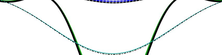
Figure (3) Radiation intensity at different polar angles (black solid line) and contributions from
the charge (green solid line), and the electric quadrupole moment (black, red and blue dashed lines)
with the following parameters: β = 0.5, d = 1mm, a = d/2, ρ̄0 = 300nm, ` = 1000, N = 50, Φ = π2 .
ηq = ω/ε ηµ = `λc /λ ηQ0 = ρ̄20 /h2eff ηQ1 = `2 λ2c /ρ̄20 ηQ2 = N 2 `2 λ2c /ρ̄20 N
1.95 × 10⁻¹⁰ 1.95 × 10⁻⁷ 2.67 × 10⁻⁶ 1.69 × 10⁻⁶ 4.22 × 10⁻³ 50
ηµµ = ηµ2 ηµQ0 = ηµ ηQ0 ηµQ1 = ηµ ηQ1 ηµQ2 = ηµ ηQ2 ` ρ̄0 , µm
3.8 × 10⁻¹⁴ 5.2 × 10⁻¹³ 3.29 × 10⁻¹³ 8.23 × 10⁻¹⁰ 1000 0.3
ηQ00 = ηQ0 ηQ0 ηQ01 = ηQ0 ηQ1 ηQ02 = ηQ0 ηQ2 ηQ11 = ηQ1 ηQ1 ηQ12 = ηQ1 ηQ2 ηQ22 = ηQ2 ηQ2
7.11 × 10⁻¹² 4.5 × 10⁻¹² 1.13 × 10⁻⁸ 2.85 × 10⁻¹² 7.13 × 10⁻⁹ 1.78 × 10⁻⁵
Table (1) Dimensionless parameters of the model which correspond to the Figure 2. The dynamical
non-paraxial contribution ηQ2 is the biggest one.
can be considered as next-to-leading order corrections which are at least two orders of magnitude
smaller (we plot the corresponding curves in figures 2 and 3 just to demonstrate their shapes).
Studies of the radiation from classical beams show that horizontal and vertical beam spreading
lead to some modifications of the spectral line [40]. The horizontal spreading of the beam shifts
the spectral line towards lower frequencies while the vertical spreading results in the opposite shift.
A combination of both spreading types results in a broadening of the spectral line. Here we show
that quantum coherence of the wave packet may lead to a different behavior. Namely, despite the
vertical-horizontal spreading of the wave-packet, the resulting spectral line does not demonstrate a
broadening until the quadrupole-quadrupole corrections come into play, which is the case for long
gratings with N
Nmax only.
Such a stabilization of the line width can be explained using (58), (59) and properties of the
function F (ω). First of all, instead of a full width at half maximum (FWHM) one can consider a
full width between zeros of the spectral curves. Zeros of the interference contributions are defined
by zeros of the kernel F itself+ . Therefore, all contributions (55)-(61) have the same full width
+
In a vicinity of a zero ω0 , F (ω0 ) = 0, the kernel F can be factorized as F (ω) = (ω − ω0 )Fres (ω). (ω − ω0 ) is a real
function therefore in (58), (59) the same factorization can be applied to the radiation intensitiesSmith-Purcell radiation of a vortex electron 19
between zeros of the spectral curves (in Fig. 2 an example of these coinciding zeros near the spectral
maximum is presented). This strongly restricts the possible broadening of the spectral line and at
large N all contributions (55)-(61) tend to have the same width.
The quadrupole-quadrupole corrections dWQ1 Q2 and dWQ2 Q2 contain only derivatives of the
kernel F . As a result, zeros of their spectral curves (in a vicinity of the maximum) disappear and
the corresponding lines demonstrate a broadening (see figure 4). Importantly, if one takes into
account these contributions then the next corrections of the same order should also be taken into
account, such as interference of the charge with the octupole magnetic moment, with 16pole electric
moment and so forth (see (10)). However, the octupole magnetic moment contribution has the same
symmetry as the magnetic momentum contribution, thus vanishing in the zenith direction. Regarding
dWe16p contribution, because it is the interference term the zeros of the kernel F will also prevent
a broadening of the corresponding spectral line. As a result, the next corrections that may lead to
a broadening are only the quadrupole-quadrupole ones. Therefore figure 4 and table 2 contain all
necessary terms.
1.5
(arb. units)
1.0 dWe
dW
dW+dW QQ
dωdΩ
d 2W
0.5
0.0
0.925 0.930 0.935 0.940 0.945 0.950 0.955 0.960
ω (THz)
Figure (4) Broadening of the spectral line due to the quadrupole-quadrupole corrections to the S-P
radiation. The grating period d = 1 mm, β = 0.5, a = d/2, ρ̄0 = 300nm, ` = 1000, Φ = Θ = π2 .
Number of strips N = 150.
Numerical studies of the spectral lines reveal not only an absence of the broadening, but even
a slight narrowing of the lines due to the charge-quadrupole interference. The FWHM for various
grating lengths are presented in Table 2 where a narrowing of the line (Charge+LO corrections
column) can be seen. When N > 100 the quadrupole-quadrupole contributions become importantSmith-Purcell radiation of a vortex electron 20
Charge Charge+LO corrections Charge+LO+NLO corrections
∆ω, THz, N=25 0.033408 0.033381 0.033383
narrowing, %, N=25 −0.081 −0.077
∆ω, THz, N=50 0.016710 0.016658 0.016668
narrowing, %, N=50 -0.31 -0.25
∆ω, THz, N=100 0.0083557 0.0082679 0.0083364
narrowing, %, N=100 -1.05 -0.23
∆ω, THz, N=150 0.0055705 0.0054660 0.0056454
narrowing, %, N=150 -1.8 +1.3 (broadening)
Table (2) Comparison of the FWHM for the charge radiation, with the interference terms included
(line narrowing) and with the quadratic terms included (line broadening). The grating period d = 1
mm, β = 0.5, ρ̄0 = 0.3µm, ` = 1000, h = 0.39 mm, Φ = π2 , Θ = π2
(Charge+LO+NLO corrections column of Table 2) and when N > 150 broadening due to the
horizontal-vertical spreading surpasses the narrowing. Thus, for N < 100 we can safely compute
dW = dWe + dWeQ2 for parameters from Table 1.
A physical reason for the line narrowing is also spreading of the wave packet. Indeed, the natural
width of the spectral line ∆ω is related to the time scale of the radiation process ∆t by a following
uncertainty relation:
1
∆ω ∼ . (66)
∆t
Due to the packet spreading, its interaction with the strips lasts longer, especially at the end of the
long grating with dNmax
zR , and so ∆t(z) grows. In other words, the spreading slightly increases
the radiation formation length.
4.2. Angular distributions at the Smith-Purcell wavelength
Let us denote
2π 2π g
ωg = = −1
, g = 1, 2, 3, ...
λg d (β − cos Θ)
then |F |2 contains a Fejér kernel
sin2 N dΘ 1
X
2
FN (ω) = − −− → 2π δ (dω(1/β − cos Θ) − dωg (1/β − cos Θ)) =
N sin2 dΘ2 1 N →∞
g
X 2πg X ωg
= δ (ω − ωg ) = δ (ω − ωg ) (67)
g
gd(β −1 − cos Θ) g
g
which can be used to integrate over frequencies in a vicinity of the resonant one. For the charge,
the charge-dipole and the charge-Q0 contributions, the Fejér kernel can be substituted by a deltaSmith-Purcell radiation of a vortex electron 21
function when N is large. For a grating of finite length with N strips the spectral line has a width
proportional to 1/N . The angular distributions of the charge radiation and of the charge-dipole
radiation for the main diffraction order g = 1 read
d2 ω13
dWee 2 aπ 2ω1 y
q
2 2 2 2
= N 2 sin exp − 1 + β γ cos Φ sin Θ
dΩ π d βγ
cos2 Θ + 2βγ 2 cos2 Φ cos Θ sin2 Θ + sin2 Φ sin2 Θ + β 2 γ 4 cos2 Φ sin4 Θ
× , (68)
β 2 γ 2 (1 + β 2 γ 2 cos2 Φ sin2 Θ)
`d2 ω14 1
dWeµ 2 πa 2ω1 y
q
2 2 2 2
=N sin exp − 1 + β γ cos Φ sin Θ
dΩ mπ 2 β 2 γ 2 d βγ
cos Φ sin Θ βγ 2 sin2 Θ + cos Θ
× p . (69)
1 + β 2 γ 2 cos2 Φ sin2 Θ
Both the intensities linearly increase with N .
Integration of the non-paraxial terms, dWeQ1 and dWeQ2 , is more tricky. First we note that
at large N the spectral factors FeQj are concentrated near the Smith-Purcell frequency and have a
width ∼ 1/N . FeQ1 is approximately an odd function and FeQ2 is an even function of ω − ω1 (see Fig.
2). Therefore FeQ1 produces a shift of the spectral maximum, whereas FeQ2 amplifies the intensity.
At large N these spectral factors are related with the Fejér kernel and its derivatives.
For instance, the charge-Q2 intensity has the following factor at large N :
2 3 2 2 aΘ1
FeQ2 = 2d N Θ1 sin FN (ω) + O(N ) (70)
2
which is just proportional to the Fejér kernel and can be substituted by a delta-function. As a result,
the dynamically enhanced charge-quadrupole interference term dWeQ2 /dΩ reads
2
dWeQ2 2 λc 1 f2 (N ) dWee
=` . (71)
dΩ ρ̄0 3β 4 γ 4 λ21 dΩ
Expectedly, this dynamical contribution is suppressed in the relativistic case, γ
1, when the
spreading is marginal. Here
aπ
f2 (N ) = 3πad cot + 3π 2 a2 + 3π ad(N − 1) + d2 (π 2 (2N 2 − 3N + 1) − 3) ≈
d
≈ 2π 2 d2 N 2 when N
1. (72)
Note that
f2 (N ) 2π 2 d2 N 2
≈ ∼ 2π 2 N 2 at N
1,
λ21 λ21
as λ1 ∼ d everywhere except Θ → 0. (73)
As a result, 2
dWeQ2 dWee λc
/ ∼ `2 N 2 , N
1.
dΩ dΩ ρ̄0Smith-Purcell radiation of a vortex electron 22
Importantly, 1/λ21 (Θ) is the only additional angle-dependent factor in dWeQ2 compared to dWee , so
the dynamical contribution is increased for smaller wavelengths – that is, for smaller emission angles,
Θ → 0. Namely, at β ≈ 0.5 we have
dWeQ2 (Θ = 0)
≈ 4. (74)
dWeQ2 (Θ = π/2)
A large N asymptotic of the charge-Q1 spectral factor reads
2 aΘ1
FeQ1 = −N ω sin FN0 (ω) + O(1) , (75)
2
where a derivative of the Fejér kernel appears
dΘ1 sin dN2Θ1 cot dΘ2 1 sin dN2Θ1 − N cos dN Θ1
X ωg
0
FN (ω) = 2
−−−→ δ 0 (ω − ωg ) .
N ω sin2 dΘ2 1
N →∞ g
Integration of (65) when g = 1 can be done using a substitution of FN0 (ω) by a derivative of a
delta-function
−2yω
Z
dWeQ1 2 aΘ1
q
= −N ω1 exp 2 2 2 2
1 + β γ cos Φ sin Θ PeQj (kx , y, ω)ω sin δ 0 (ω − ωg ) dω =
dΩ βγ 2
−2yω aΘ1
q
2 2 2 2 2
N ω1 ∂ω exp 1 + β γ cos Φ sin Θ PeQj (kx , y, ω)ω sin .
βγ 2 ω→ω1
Using explicit expressions of the radiation intensities one can isolate the dimensionless
parameters related with the quadrupole contribution. From Eq.(71), one can find ηQ2 , while ηQ1
and ηQ2 can be extracted from the ratios dWeQj /dWee :
ρ̄20 2
dWeQ0 2 λc h
= 2 P1 (β, Θ, Φ) + ` 2 P2 β, , Θ, Φ , (76)
dWee heff ρ̄0 d
2
dWeQ1 2 λc h
= ` 2 P3 β, , Θ, Φ , (77)
dWee ρ̄0 d
where P1,2,3 are some smooth functions. One can identify three parameters (16), (17). Note that
dWeQ0
dWee
contains a linear combination of independent parameters ηQ0 and ηQ1 , which we split for
a convenience. For ultra-relativistic energies, all corrections from the quadrupole radiation are
suppressed.
In Figure 5 we plot an azimuthal distribution of the radiation intensity at λ = 2 mm and compare
different contributions to the total radiation intensity. We fix the impact parameter and initial radius
of the wave packet and consider two cases: ` = 1000, N = 50 and ` = 100, N = 500. In both cases
the maximal number of strips for a given impact parameter, OAM and the initial radius ρ̄0 is used.
A larger grating length corresponds to the smaller angular momentum ` = 100. A scaling invarianceSmith-Purcell radiation of a vortex electron 23
` → `, N → −1 N of the quadrupole correction dWeQ2 /dWee ∼ ηQ2 can be observed in Figure 5.
In other words, large OAM lead to a quick spreading and require short gratings, while small OAM
result in a relatively slow spreading and allow one to use longer gratings. At the same time, other
corrections – in particular from the magnetic moment – depend on ` only. Their observation requires
the largest possible OAM (` ∼ 103 and higher) and Φ 6= π/2.
Note that for β = 0.5, the charge and the charge-quadrupole contributions have almost the
same azimuthal dependence (which is defined mostly by the exponential factor). The charge-magnetic
moment contribution yields the small azimuthal asymmetry. The analysis of Ref.[2] seems reasonable
for the case of the Smith-Purcell radiation too. In the case of THz radiation (λ ∼ 1mm) this effect
is almost unobservable (see figure 5 and Table 1). An asymmetry of the order of 0.1 % can be seen
for infrared S-P radiation, λ ∼ 1 µm, which could in principle be measured.
4.3. Dynamical enhancement of the quadrupole contribution
Equations (71), (72) show that dWeQ2 contribution has a qubic growth with the number of strips
compared to the linear growth of dWee . This is due to constructive interference of the quadrupole
radiation from each strip, taken into account that the quadrupole moment is increased (quadratically)
because of the spreading. Recall that the maximal grating length (interaction length) and the number
of strips are limited by (5) to guarantee that the mean wave packet radius ρ̄(t) stays smaller than
the impact parameter h.
A large impact parameter h should be chosen to obtain a large Nmax , therefore we consider
3
ρ̄0 /h
1 and thus approximately Nmax ∝ h3 . At the same time, the radiation intensity
decreases exponentially with the large impact parameters. Taking the maximal number of strips, the
dependence of the charge-quadrupole interference term dWeQ2 on the impact parameter reads
ρ̄0 d 2h
3 − heff
dWeQ2 [ρ, `, h, Nmax (ρ, `, h)] ∝ h e . (78)
` λc h5eff
The maximum of this contribution defines the optimal impact parameter
3
hopt ≈ heff ∼ heff .
2
Note that dWeQ2 is proportional to ρ̄0 /` when N takes its maximal value (5). That is, a wide packet
with a small OAM (recall the corresponding lower bound (28)) can be chosen to simplify experimental
studies of the S-P radiation from the vortex electrons.
In figure 6 the behavior of the radiation intensity is shown for the optimal value of h and
Nmax (h) = 700. Two cases of OAM, ` = 150 and ` = 100, were considered. The maximal number of
strips was calculated for the larger OAM. The diffraction time is inversely proportional to `, therefore
a grating optimal for a wave packet with ` = 150 can be used also in the case of ` < 150. In this
case a factor `2 /1502 reduces the charge-quadrupole radiation intensity dWeQ2 .Smith-Purcell radiation of a vortex electron 24
0.25
0.20
(arb. units)
0.15
dWe 104 dWeQ1
0.10 dW dWeQ2
105 dWeμ
dW
dΩ
0.05 104dWeQ0
0.00
0 π π
2
Φ
(a) ` = 1000, N = 50
2.5
2.0
(arb. units)
1.5
1.0
dWe 106 dWeQ1
dW dWeQ2
106 dWeμ
dW
dΩ
0.5
104dWeQ0
0.0
0 π π
2
Φ
(b) ` = 100, N = 500
Figure (5) Azimuthal distribution of the radiation intensity (black solid line) and contributions from
the charge (green solid line), the magnetic moment (cyan dashed line), and the electric quadrupole
moment (black, red and blue dashed lines) with the following parameters: β = 0.5, λ = 2mm,
d = 1mm, a = d/2. The number of strips N is maximal in each subfigure for the given OAM, the
impact parameter h = 0.13mm and ρ̄0 = 0.3 µm.
The non-linear dependence of the S-P radiation on the number of strips or on the length
of the grating due to the increasing quadrupole moment is clearly seen in figure 6. If observed
experimentally, such a non-linear dependence would serve as a hallmark for a non-paraxial regime of
electromagnetic radiation, in which an electron packet emits photons as if its charge were smeared
over all the coherence length, somewhat similar to a multi-particle beam but with a total charge e.
Another possibility to detect this effect is to change OAM for the same diffraction grating and the
same scattering geometry and to study corresponding modifications of the radiation intensity.Smith-Purcell radiation of a vortex electron 25
π
Φ =Θ =
2
1.4
dW, l=150
1.2
dW, l=100
(arb. units)
1.0
dWe
0.8 dWeQ2 , l=150
0.6 dWeQ2 , l=100
dW
dΩ
0.4
0.2
0.0
0 100 200 300 400 500 600 700
N
Figure (6) Radiation intensity at vertical plane for various number of strips N < 700. The number
of strips N = 700 is maximal given that the impact parameter h = 3heff /2 = 27 µm, velocity β = 0.5,
period d = 0.1 mm and the initial mean radius ρ̄0 = 300 nm.
An additional possibility to detect the charge-quadrupole contribution follows from a polar
dependence in (71). In most cases, the total radiation intensity is approximately dW = dWe + dWeQ2
because other corrections are at least 2 orders of magnitude smaller than dWeQ2 . In the case of large
N and Φ = π2 , the maximum of the radiation intensity with respect to the polar angle Θ can be
found by maximization of the following expression:
−2h ηQ2 d2
dW ∝ e heff h−3 −5
eff + δheff , δ= . (79)
6 γ 2β 2
To begin with the polar angle of maximal intensity for the charge radiation Θe we just put δ = 0
which gives heff (Θe ) = 2h/3 from a linear equation. A non-zero δ leads to the cubic equation. We
use Cardano’s formula and assume δ small to calculate the first order correction
δ
heff (Θ) = heff (Θe ) − . (80)
h
Next, we write effective impact parameters explicitly in terms of the polar angle
βγd δ
(cos(Θe ) − cos(Θe + δΘ)) = −
2π hYou can also read