Geometric secret sharing in a model of Hawking radiation
←
→
Page content transcription
If your browser does not render page correctly, please read the page content below
Published for SISSA by          Springer
                                                                      Received: October 23, 2020
                                                                    Accepted: December 14, 2020
                                                                     Published: January 27, 2021

Geometric secret sharing in a model of Hawking
radiation

                                                                                                     JHEP01(2021)177
Vijay Balasubramanian,a,b Arjun Kar,a Onkar Parrikar,c Gábor Sárosid and
Tomonori Ugajina
a
  David Rittenhouse Laboratory, University of Pennsylvania,
  209 S.33rd Street, Philadelphia, PA 19104, U.S.A.
b
  Theoretische Natuurkunde, Vrije Universiteit Brussel (VUB), and International Solvay Institutes,
  Pleinlaan 2, B-1050 Brussels, Belgium
c
  Stanford Institute for Theoretical Physics, Stanford University,
  Stanford, CA 94305, U.S.A.
d
  Theoretical Physics Department, CERN,
  1211 Geneva 23, Switzerland
    E-mail: vijay@physics.upenn.edu, arjunkar@sas.upenn.edu,
    parrikar@stanford.edu, gabor.sarosi@cern.ch, loop.diagram@gmail.com

Abstract: We consider a black hole in three dimensional AdS space entangled with an
auxiliary radiation system. We model the microstates of the black hole in terms of a
field theory living on an end of the world brane behind the horizon, and allow this field
theory to itself have a holographic dual geometry. This geometry is also a black hole
since entanglement of the microstates with the radiation leaves them in a mixed state.
This “inception black hole” can be purified by entanglement through a wormhole with
an auxiliary system which is naturally identified with the external radiation, giving a
realization of the ER=EPR scenario. In this context, we propose an extension of the Ryu-
Takayanagi (RT) formula, in which extremal surfaces computing entanglement entropy are
allowed to pass through the brane into its dual geometry. This new rule reproduces the
Page curve for evaporating black holes, consistently with the recently proposed “island
formula”. We then separate the radiation system into pieces. Our extended RT rule shows
that the entanglement wedge of the union of radiation subsystems covers the black hole
interior at late times, but the union of entanglement wedges of the subsystems may not.
This result points to a secret sharing scheme in Hawking radiation wherein reconstruction
of certain regions in the interior is impossible with any subsystem of the radiation, but
possible with all of it.

Keywords: AdS-CFT Correspondence, Black Holes

ArXiv ePrint: 2003.05448

Open Access, c The Authors.
                                                       https://doi.org/10.1007/JHEP01(2021)177
Article funded by SCOAP3 .
Contents
1 Introduction 1
2 Holographic inception for black hole microstates 4
2.1 Inception for microstates 5
2.2 Quantifying the inception theory 6
2.3 Reproducing the Page curve: microstates, islands, and inception 11
JHEP01(2021)177
2.4 Details of the evaporation protocol 14
2.5 Proof by replica trick 15
3 Secret sharing in Hawking radiation 16
3.1 Covering space construction of multiboundary wormholes: review 17
3.2 Secret sharing between two radiation subsystems 19
3.3 Other eyelands 27
4 Discussion 29
A Useful formulas for identifications on the upper half plane 32
B Partial islands for the three-boundary inception geometry 33
B.1 BTZ subregion entropy at finite cutoff 33
B.2 Moduli and geodesics in covering space 35
B.3 An eyeland from inception 38
C Long wormholes from multiboundary black holes with EOW branes 38
C.1 Euclidean geometry 39
C.2 Lorentzian geometry 40
1 Introduction
The semiclassical calculation of Hawking [1] predicts that pure states of quantum theories
can collapse to make black holes and then evaporate into mixed states, thus destroying in-
formation, a scenario which is forbidden if quantum mechanics is correct. By contrast, the
AdS/CFT correspondence suggests that information can be recovered from black holes be-
cause the whole spacetime is dual to a unitary CFT. Many authors have suggested that the
mechanism for information recovery from black holes is entanglement of Hawking quanta
with the interior microstate. Naively quantifying this entanglement as the von Neumann
entropy of effective field theory on the black hole background leads to a contradiction —
the entanglement seems to grow continuously with time, which is impossible if there are
a finite number of black hole microstates in the first place with which the radiation may
–1–be entangled. In flat space, where black holes evaporate completely, the entropy of the
radiation must decline back to zero eventually, while in AdS space, where large black holes
come into equilibrium with the radiation, the entanglement entropy should level off at a
plateau. The time at which the entropy growth stops is called the Page time [2].
Recent work [3] has clarified the problem in the simplified setting of two-dimensional
Jackiw-Teitelboim gravity coupled to a non-gravitating 2d CFT representing radiation
degrees of freedom distant from the black hole. This work suggests that the rectification
of the Page curve is already visible in the semiclassical theory if the entanglement entropy
SA of Hawking radiation collected in a weakly- or non- gravitating region A is actually
computed by a new “island formula”:
JHEP01(2021)177
Area(∂B) eff
SA = min ext + SAB (1.1)
B 4GN
where B is an “island” in the gravitating region, Area(∂B) is the area of the boundary
of the island, and SAB eff is the effective field theory entanglement entropy of quanta in
the union of the regions A and B. This formula was inspired by the quantum extremal
surface formula for holographic entanglement entropy [4], and the papers [5, 6] showing
new quantum extremal surfaces inside evaporating black holes. Technically, the authors
of [3] demonstrated their ideas by taking the radiation CFT to be holographically dual to a
three dimensional classical gravity in which entropies of subregions could be computed by
the Ryu-Takayanagi (RT) formula [7] in one higher dimension. In this context, the island
formula ensures that entropy growth in Hawking radiation terminates at the Page time.
Further work has demonstrated that the island formula follows when the radiation entropy
is computed via the replica trick, provided certain novel Euclidean wormholes between
replicas are included [8, 9].1
In this paper, we examine these ideas in three dimensions with a negative cosmological
constant, while following [9, 17–19] to model black hole microstates as excitations of an
End-of-the-World (EOW) brane that truncates the geometry behind the horizon of an
eternal black hole (figures 1a,b). Because we are working with 3d gravity, the EOW
brane is 2-dimensional. The EOW brane has a Hilbert space containing the black hole
microstates, and we imagine this Hilbert space comes from a quantum theory living on the
brane. We take this brane theory to itself be a (deformation of a) 2d conformal field theory
(the Brane CFT, which is distinct from the CFT living on the asymptotic boundary of the
spacetime). We then consider the holographic dual to the Brane CFT, “filling in” the EOW
brane to give a complete 3d geometry. In the region behind the brane there is a different
cosmological constant related to the central charge of the Brane CFT, which is in turn
associated to the number of black hole microstates. We call the 3d geometry behind the
brane the Inception Geometry.2 As an example, consider a situation where k microstates
(in some basis) are maximally entangled with external radiation quanta. In this case, the
1
See [10–16] for further work on quantum extremal islands in evaporating black holes.
2
This terminology is inspired by the 2010 film Inception (spoilers ahead). In the context of the film,
“inception” refers to planting an idea in someone’s mind. Here we use it instead to refer to the dream
within a dream, as we have constructed a geometry within a geometry.
–2–B A EOW A
(a) (b)
ID A
JHEP01(2021)177
(c)
Figure 1. (a) The time-reflection-symmetric slice of the eternal BTZ black hole is a wormhole
between two asymptotic regions, A and B. The dashed circle is the bifurcate horizon. This geometry
is dual to the thermofield double state. (b) The two-sided wormhole with one side truncated and
replaced with an EOW brane (red circle) at a finite distance from the bifurcate horizon. In our model
the EOW brane has an internal state structure which matches that of a 2d CFT. (c) The EOW
brane can be replaced with its holographic dual geometry. When the brane CFT is in a thermal
state above the Hawking-Page transition, this geometry is a black hole within the inception disk
(ID, gray) which is glued to the original geometry at the location of the brane (dashed red circle).
The entropy associated with the brane is proportional to the area of the black hole horizon in the
inception disk. This “inception horizon”(dashed blue circle) is an extremal surface homologous
to the asymptotic region A. As such, it competes with the usual bifurcate horizon (dashed black
circle) when we use the RT formula to search for the minimal surface which computes the entropy
of A. In other words, the homology constraint in the RT formula can be satisfied by pulling curves
through the circle where the inception disk meets the real geometry.
state of the Brane CFT will be thermal; thus the Inception Geometry will itself contain a
black hole. Then the total geometry has two horizons, one in the real space and one in the
inception space (figure 1c). We will realize this scenario by imposing a modified version
of the Israel junction conditions [20] to glue the inception geometry to the real one. This
procedure will lead us to the most general way to glue two BTZ black holes with different
temperatures, curvature radii, and Newton’s constant, and no additional non-holographic
stress energy on the gluing surface.
In this context, we propose a new form of the Ryu-Takayanagi (RT) formula, whereby
entanglement entropy in the CFT dual to AdS space is computed by the area of extremal
surfaces that are allowed to pass through the EOW brane into the Inception Geometry,
and motivate the new rule by setting up a replica derivation. The surfaces computed with
this form of the RT formula are models of Quantum Extremal Surfaces [4–6], where the
bulk effective field theory contribution to the quantum gravity entropy is modeled by a
contribution from the inception geometry. We apply our prescription to a setting where
EOW brane microstates are maximally entangled with radiation that has escaped through
–3–a transparent AdS3 boundary (marked A in figure 1c) into an external reservoir. The CFT
dual to the AdS geometry captures the physics of the black hole microstates but not the
emitted radiation, and so it must display an entanglement entropy computed by the area
of extremal surfaces homologous to the AdS boundary. In our extended RT prescription
there are two competing extremal surfaces satisfying this homology condition: the horizon
of the real black hole, and the horizon of the inception black hole, shown in figure 1c. The
smaller area gives the entanglement entropy. We will see that this prescription recovers
the predicted Page behavior of Hawking radiation.
Our proposal helps to uncover new aspects of information recovery from Hawking ra-
diation. First, we can purify the inception black hole by entanglement of the microstates
JHEP01(2021)177
through a wormhole with an auxiliary system, which is naturally identified with the external
radiation. This construction gives a realization of the ER=EPR idea [21]. Furthermore,
we can split the auxiliary system (or, equivalently, the radiation) into multiple distinct
parts. Such a split can be modeled by purifying the inception black hole with a multi-
boundary wormhole [22–24]. Each leg of the wormhole corresponds to a different part of
the Hawking radiation. We focus in particular on a case where the radiation is split into
two parts corresponding to early and late time Hawking radiation which will be naturally
separated by great distances on any equal time slice, and thus will not directly interact.
By studying our extended RT prescription in the total geometry (real + inception) we find
a new class of extremal surfaces homologous to the spacetime boundaries (the “infalling
geodesics”) that do not coincide with horizons (see figure 9). The existence of these new
extremal surfaces has an interesting consequence: the entanglement wedge of any part of
the radiation contains a part of the interior of real black hole. However, there can be a
region inside the black hole which is not in the union of the entanglement wedges of any set
of subsystems of the radiation, even though it is in the entanglement wedge of the union
of subsystems.3 This missing region corresponds to a shared secret that is embedded in
the entanglement between radiation subsystems, and is only recoverable if we have access
to all of them at the same time. In this sense, Hawking radiation implements a quantum
secret sharing scheme.
2 Holographic inception for black hole microstates
Consider the eternal BTZ black hole. On the time-reflection-symmetric slice this geometry
has a spatial section with two asymptotic AdS3 regions separated by a horizon (figure 1a)
— i.e., it is a two-boundary wormhole which acts like a black hole when observed from
outside the horizon. To set up the Hawking paradox we need two ingredients: (a) a model
of the microstates, and (b) a model of the radiation system. We follow the trick of [9, 17, 19]
to model the microstates by an End-of-the-World (EOW) brane placed behind the horizon.
Schematically, the EOW brane cuts off the eternal black hole geometry, removing the second
asymptotic region (figure 1b). Modeling the radiation is tricky because the AdS geometry
acts as a box confining finite energy particles, so that the Hawking quanta will not escape,
and rather come to equilibrium with the black hole. This is awkward because if they remain
3
A similar observation was made in [14] in the context of the doubly holographic model of [3].
–4–in the gravitating geometry, their entanglement entropy should include a quantum gravity
component that is difficult to compute. We will follow [5, 6, 25] to avoid this difficulty by
imagining transparent boundary conditions at the AdS boundary that allow radiation to
be collected in a non-gravitating reservoir just outside the AdS boundary.
Suppose that the black hole has formed from collapse of a shell of matter dropped in
from the AdS boundary. Then, at early times no Hawking quanta have been collected in
the reservoir. After the black hole forms, it radiates and the number of quanta collected in
the reservoir increases. Eventually we have a black hole of a certain horizon area entangled
with radiation. We will model the Hawking quanta at a given time as occupying a k-
dimensional subspace of the reservoir Hilbert space (HR ) which is maximally entangled
JHEP01(2021)177
with a k-dimensional subspace of the black hole microstates. A unitary transformation can
distill the entangled part of the microstate Hilbert space into a separate factor HB . We
can then write the total state in terms of |iiR ∈ HR entangled with |ψi iB ∈ HB as4
k
X
|ψi = |iiR ⊗ |ψi iB . (2.1)
i=1
When k > eSBH the states |ψi iB cannot be orthogonal because the microstate Hilbert
space has dimension eSBH , where SBH is the coarse-grained black hole entropy. But when
k < eSBH , we can take the |ψi iB to be approximately orthogonal. We can understand this
orthogonality conceptually as follows. Imagine a black hole in a particular microstate, and
let it radiate some quanta. Each possible radiated configuration |ii should be in a product
with a different underlying microstate |ψi i. Since the final state will be a superposition of
such tensor products, it has the general form (2.1). Given the chaotic dynamics expected
for black holes, it is reasonable to assume that the |ψi i will be random vectors in HB . When
k is small, the required number of such random |ψi i is much smaller than the dimension
of the microstate Hilbert space, and so they should be orthogonal with high probability.
2.1 Inception for microstates
To gain further insight, the authors of [3] used a trick: they imagined that the matter
fields traveling through the black hole background and in the radiation reservoir formed
a conformal field theory with a holographic dual. We will instead take the theory on the
EOW brane to be (a deformation of) a conformal field theory, the brane CFT. This brane
CFT is different from the CFT living on the asymptotic boundary of AdS, and in particular
has a different central charge (see details in section 2.2). In fact, there is reason to expect
in string theory that the microscopic description of black hole microstates may generally
occur through such CFTs associated to D-brane sources (e.g., besides [28] and [29] see [30]
for examples involving charged black holes in AdS5 ). We will then assume that this brane
CFT admits its own holographic dual. The equal time slice of this dual theory will be
a two-dimensional disk “filling in” the EOW brane which lives on its boundary. We will
call this the “Inception Disk”. Since the states of the EOW brane are entangled with
the radiation, tracing out the radiation will leave the brane CFT in an approximately
4
Such states were previously considered in the context of black hole evaporation in [26, 27].
–5–thermal state, which is dual to a black hole in the Inception Disk (figure 1c). If the EOW
microstates are maximally entangled with k radiation quanta, the entropy of the inception
black hole will be log k.
Thus, the total system is now described by a single three-dimensional geometry in
which the cosmological constant changes across the EOW surface, since the central charge of
the EOW brane CFT is different from the central charge of the CFT on the AdS boundary.
In addition, there are two horizons. The first, associated to the asymptotic observers, is the
original one of the black hole. The second, associated to the microstates and any observer
who directly interacts with them in the black hole interior, is the inception horizon. We
JHEP01(2021)177
propose that the standard Ryu-Takayanagi prescription for entanglement entropies can be
applied in the total geometry with extremal surfaces traveling into the inception region as
necessary, subject to a refraction condition because of the changing cosmological constant,
and to a condition that they are homologous in the complete geometry to the region whose
entanglement entropy we are trying to compute. Such surfaces can be thought of as models
of Quantum Extremal Surfaces if we think about the bulk effective field theory contribution
to the generalized entropy as the entropy of the brane segment that is captured by the part
of the RT surface in the real side of the geometry. This entropy of the brane segment is
geometrized by holographic inception and captured by the piece of the RT surface living
in the inception side of the geometry. We will argue for this rule in such glued geometries
using the replica trick in section 2.5.
2.2 Quantifying the inception theory
Strictly speaking, the EOW brane theory does not have to be a CFT all the way into the
ultraviolet, and can be an irrelevant deformation of a CFT that introduces a cutoff on the
spectrum, provided that the complete brane Hilbert space has at least eSBH dimensions. In
practical terms, this means that the holographic dual of the EOW brane in the inception
disk can have a finite cutoff near its boundary, and can perhaps be understood as a T T̄
deformation of a CFT [31]. This freedom will be important for physically gluing the original
black hole to the inception geometry.
In a top-down approach we would derive the theory of the microstates and its holo-
graphic dual from the underlying quantum gravity. For example, if the black hole were
created by a collection of intersecting D-branes, we would have to work out their effective
theory. We will instead consider consistency conditions that the inception geometry must
satisfy: (1) it must produce a “long wormhole”5 region in the black hole interior leading
to a second horizon, (2) it must have two adjustable parameters for the masses of the real
and inception black holes in order to allow a tunable amount of entanglement with the
radiation reservoir, and (3) the total geometry must solve the equations of motion so that
we can define a generalization of the Ryu-Takayanagi formula.
We could follow several strategies to achieve these consistency conditions while gluing
together black hole geometries with different temperatures. We will take an approach in
5
By long wormhole we mean a wormhole which is lengthier than a standard wormhole and can have two
interior horizons; in our context, such wormholes appear when we perform inception on an EOW brane.
–6–which the Newton constant in the real and inception geometries are different. This is
natural because the theory dual to the EOW brane can certainly have parameters that are
different from those of the real spacetime. With this approach we will find that the entire
stress energy on the EOW brane can be taken to be the holographic stress tensor coming
from the inception disc. Then an “evaporation protocol” that changes the horizon area of
the inception black hole to reflect varying entanglement of the EOW brane with radiation
will also have to vary the inception curvature scale and Newton constant. An alternative
approach is to allow the EOW brane to contain a non-holographic component in its stress-
energy, or non-trivial topology behind the horizon. In these settings, which have more
parameters, it is possible to define an evaporation protocol in which the curvature scale and
JHEP01(2021)177
Newton constant in the inception geometry remain fixed as we increase the entanglement
with radiation. We will analyze the simplest scenario without such additional parameters,
and will argue that all these models give similar physical results for the Page transition
and secret sharing in Hawking radiation, essentially because the inception geometry is a
robust representation of the overall entanglement structure of the states, and does not seek
to capture the detailed properties.
Details of the inception geometry. The physical and EOW brane CFTs are allowed to
have different parameters, such as their central charges. Thus their holographic duals will
have different curvature radii and Newton constants. We will denote quantities associated
to the inception geometry with a prime: e.g., the original AdS radius will be ` and the
inception AdS radius will be `0 .
The original (Euclidean) black hole geometry is just described by the BTZ metric,
dr2
ds2 = f (r)dτ 2 + + r2 dϕ2 , (2.2)
f (r)
r2 − rh2 2π`2
f (r) = , β= , (2.3)
`2 rh
where rh is the horizon radius and β is the inverse temperature. We model microstates
following [17, 19, 32], by putting an end-of-the-world (EOW) brane behind the horizon,
and we associate a state of the inception theory with the brane. In addition to just being a
label on the brane, the choice of inception state will affect the brane trajectory. We require
the Brown-York stress tensor on the brane induced from the real side to be equal to the
stress tensor of the state we pick in the inception theory. Since we work with Neumann
boundary conditions, this condition will give an equation of motion for the brane trajectory.
When the inception theory is holographic, it is natural to impose the condition that this
stress tensor agree with the Brown-York stress tensor induced from the inception side. 6
This motivates us to glue the real and inception geometries using the following junction
6
We can choose to include holographic counterterms [33], but then we need to include them on both
sides so that we do not compare a renormalized stress tensor with a bare one. In this case they will not
change the discussion below.
–7–JHEP01(2021)177
Figure 2. Visualization of the glued Euclidean geometry. The ϕ direction is suppressed and the
partial circles are the Euclidean time circles τ and τ 0 .
conditions
hab = h0ab , (2.4)
1 1 0
Kab = 0 Kab . (2.5)
GN GN
Here hab is the induced metric and Kab is the extrinsic curvature on the gluing surface.
These conditions differ from the usual Israel junction conditions [20] in two important
way. First, we can have GN 6= G0N in which case the extrinsic curvatures must differ
across the surface. Second, we will glue the geometries so that the orientations of normal
vectors in (2.5) is the same, that is, we glue convex surfaces to convex surfaces, while
the Israel conditions glue convex surfaces to concave surfaces. In Euclidean signature,
this leads to two cigar geometries that are glued in the way depicted on figure 2.7 In
Lorentzian signature, we need to imagine the glued geometry as a folded piece of paper
when embedded in higher dimensional space (see left of figure 4), so that the real and
inception bulks are living “on top of each other”. While this choice of orientation is
required to find interesting solutions for our purposes, it is also appealing as a model of
both black hole complementarity and ER=EPR. Indeed, we can imagine that the radiation
degrees of freedom in the real CFT A are connected via ER=EPR bridges to the EOW
brane behind the horizon. When we remove radiation from A into the reservoir R, we also
“split” the bulk dual into two, and the removed ER=EPR bridges make up the inception
part of the geometry, that lives on top of the real geometry, but after the splitting, only
connects to it at the EOW brane (figure 5).
We will be interested in the situation when the microstates are entangled with the
radiation, and so the inception geometry is itself a black hole. The inception geometry is
then also given by the BTZ metric (2.2), with parameters rh0 and `0 . We will now find the
most general rotationally invariant surfaces that solve the junction conditions (2.4), (2.5)
in this case.
7
A similar Euclidean geometry was considered in [34] (see also [35] for a JT gravity version leading to
long wormholes), with a conventional convex to concave gluing. The main difference is that in our case
there is no stress tensor localized on the shell, which is possible only because the two sides of the gluing
have different parameters in their actions.
–8–We will work in Euclidean signature. The most general such surface is given by some
trajectory r(τ ). Pulling back the metric (2.2) we find that hϕϕ = r2 (τ ). Then the equation
hϕϕ = h0ϕϕ fixes the change of coordinate between the two sides to be r(τ ) = r(τ 0 ). It
is therefore useful to change the coordinate τ to r on the surface, which is a common
coordinate. After the change of coordinates we have
dτ 2 2
`4 + (r − rh2 )2
dr r(r2 − rh2 )3/2
hrr = , Kϕϕ = − r . (2.6)
`2 (r2 − rh2 ) ` `4
+ (r2 − rh2 )2
2
( dτ
dr )
JHEP01(2021)177
We can now solve the equations hrr = h0rr and Kϕϕ /GN = Kϕϕ 0 /G0 for the derivatives of
N
the real and inception gluing surfaces. After integrating, the solution is
q
r̃2 − rb2
s
rt2 − rh2
Z r
2
τ (r) = ` dr̃ (2.7)
rh2 − rb2
p
rt (r̃2 − rh2 ) r̃2 − rt2
q
r̃2 − rb2
s
2
rt − rh 02 Z r
τ 0 (r) = `02 dr̃ , (2.8)
rh02 − rb2 rt
p
(r̃2 − rh02 ) r̃2 − rt2
(the prime on τ 0 denotes inception quantity and not derivative). We have defined in the
above expressions
s s
`2 G2N rh02 − `02 G02 2
N rh `2 rh02 − `02 rh2
rt = 02 , rb = , (2.9)
2
`2 GN − `02 GN `2 − `02
dr dr
where rt corresponds to the turning point where dτ = 0, while at rb , dτ = ∞. To get a
real solution for the brane trajectory we need rb < rh , rh0 and rh , rh0 < rt . The integrals can
be given in terms of elliptic functions, but we will not need their explicit forms. To write
the EOW brane trajectory we will need the turning point rt , which is the location of the
brane on the τ = 0 slice where we continue to Lorentzian signature.
The rr component of the extrinsic curvature reads as
d2 τ
dτ 2 3`4 r `4
(r2 rh2 ) r3 rrh2
dr 2
dr 2 + − + − dτ 3
( dτ
dr ) ( ) dr
Krr = − q r , (2.10)
`4
`3 r2 − rh2 2 2 2
2 + (r − rh )
( dτ
dr )
and one can check that the solution (2.7)–(2.9) automatically satisfies the last junction
condition Krr /GN = Krr 0 /G0 .
N
It is important that a non-singular (without cusps or self-intersections) Euclidean brane
trajectory should start from the boundary and return to the boundary after reaching the
turning point rt (figure 3). For this to happen, we need that rt > rh , rh0 , which are the
origins of the Euclidean real/inception geometries, and that rt > rb (to avoid singularities).
A real trajectory in (2.7) then requires rb < rh , rh0 < rt (or just rh , rh0 < rt when rb is purely
–9–JHEP01(2021)177
Figure 3. Illustration of a healthy brane trajectory in Euclidean (left) and Lorentzian (right).
The two figures share the time reflection symmetric slice (green dotted).
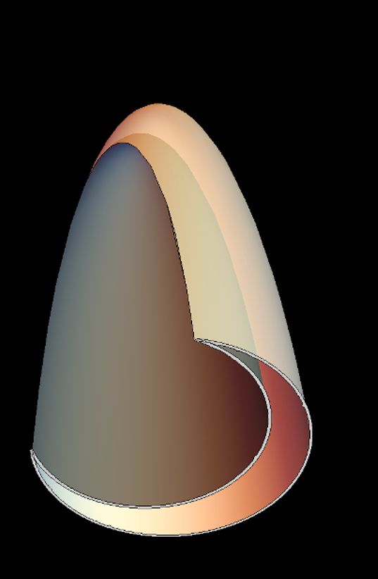
Figure 4. The maximally extended Penrose diagram of the spacetime after inception. The real
black hole spacetime (white) terminates at the EOW brane (red dashed line), then holographic
inception creates the region behind (gray). The inception region also contains a black hole, due
to the entanglement in the state (2.1). Left: since we glue convex-to-convex, we need to imagine
the diagram as a folded piece of paper. Right: the causal structure is better visualized when we
unfold the diagram. Note that a conventional convex-to-concave gluing would not lead to a long
wormhole: it would require us to delete the other side of the brane in the inception geometry.
imaginary). These inequalities give constraints on the possible choice of parameters. 8 The
spatial slice of the glued geometry is given in figure 1c, and the Penrose diagram after
continuation to Lorentzian looks like figure 4. Note that later on, we will only use the time
reflection symmetric slice of this geometry.
The solutions (2.7) include the constant tension brane (Kab = T hab ) as a special case
0
when rb = 0 or rh0 = `` rh . In this case, the brane trajectory has an elementary form [19]
s
rh
1 + `2 T 2 tan2 `2
τ
r(τ ) = rh , (2.12)
1 − `2 T 2
8
For future reference we note that we can trade the parameters G0N , `0 of the inception theory for rt and
rb . They are re-expressed as
s s
0 rh02 − rb2 0 (rh2 − rb2 )(rt2 − rh02 )
` =` , G N = GN , (2.11)
rh2 − rb2 (rh02 − rb2 )(rt2 − rh2 )
and are real when rb < rh , rh0 < rt .
– 10 –where r
G `02 − `2
T = 0 , (2.13)
`` G2 − G02
and the trajectory on the inception side is obtained by swapping primed and unprimed
parameters. One can calculate the induced metric on the brane, and it describes a Big
Bang-Big Crunch cosmology. It has a simple form if we introduce the new time coordinate
τ̂ = r`h arctan `T tan r`h2τ , in which it reads as
rh2
ds2 = (dτ̂ 2 + dϕ2 ). (2.14)
rh τ̂
(1 − `2 T 2 ) cos2
JHEP01(2021)177
`
π` π`
This is Euclidean AdS2 in global coordinates, with τ̂ ∈ − 2r ,
h 2rh
playing the role of the
global spatial coordinate of AdS2 , and ϕ playing the role of the time of AdS2 .
In the above construction, we will allow the black hole in the inception geometry to
have an entropy bigger than that of the original black hole in the real geometry. From the
microscopic perspective the logic of this scenario may seen puzzling. How is it possible to
conceive of an inception black hole with entropy bigger than the coarse-grained entropy
of the original black hole if the EOW brane theory is supposed to be modeling the black
hole microstates? Indeed, from the microscopic point of view, the brane theory modeling
the black hole microstates must have a Hilbert space dimension set by the Bekenstein-
Hawking entropy, preventing any information paradoxes. However, here we are considering
an effective field theory situation in which the entropy of the Hawking quanta seems to
rise indefinitely because subtle correlations are not included in the low-energy calculation.
From the black hole interior point of view this means that we must correspondingly imagine
that a very large Hilbert space can hide behind the black hole horizon, and that these states
are entangled with the Hawking radiation giving rise to its thermal character. In effect, this
means that in (2.1) we continue to take the microstates |ψi i to be orthogonal in the effective
description even when their number exceeds eSBH . Below, we will show that if we use this
ruse to try to generate a paradox in the effective theory, the Ryu-Takayanagi formula
extended to include the presence of the EOW brane and its dual geometry will contrive
to rescue the consistency of the theory without the need for a microscopic description, an
effect which we may refer to as entropic censorship.
2.3 Reproducing the Page curve: microstates, islands, and inception
In our geometric description of the state (2.1) (figure 1c), we can simply compute the en-
tanglement entropy of the theory on the AdS boundary by computing the Ryu-Takayanagi
(RT) formula applied to extremal surfaces homologous to the entire AdS boundary. There
are two such extremal surfaces in figure 1c — the original horizon which gives entropy SBH ,
and the inception horizon which gives entropy log k. This is related to the horizon size of
the inception black hole rh0 and the Newton constant G0N in this region through
π rh0 2πc0
log k = 0 = , (2.15)
2 GN 3β 0
– 11 –R1
R1
A A
R2
R2
JHEP01(2021)177
Figure 5. The spatial slice of the glued geometry when we purify the inception black hole with
a two boundary wormhole. Left: since we glue convex surfaces to convex surfaces, the original
boundary and the purifying systems are naturally on the same side. Right: in order to increase
clarity, we “unfold” the diagram on the left when we depict its various features.
where c0 is the central charge of the brane CFT, and β 0 is the temperature of the inception
black hole.
Clearly when k < eSBH the RT prescription selects the inception horizon as a measure
of the entanglement entropy, but when k > eSBH the original horizon is selected, giving SBH
as the entanglement entropy. In the dynamical scenario discussed above, this implies that
the entanglement entropy of the radiation in this holographic computation will increase
until it equals SBH and will plateau there. Our prescription thus reproduces the result
of the island formula [3], in which the island would have been the region between the
original horizon and the EOW brane. However, in our setup there was no need to invoke
an island. The standard prescription for holographic entanglement entropy reproduces the
result, perhaps giving an alternative justification for it in our three-dimensional setting.
From a slightly different perspective, we can regard the “islands” of [3] as regions of space
disconnected from the AdS boundary that can be reconstructed due to their entanglement
with the radiation. We will see that when enough radiation has been collected, an “island”
in this sense appears because the entire region behind the black hole horizon becomes part
of the entanglement wedge of the radiation.
As discussed above, the inception geometry contains a black hole, and is dual to a
thermal state in the brane CFT. We can purify this state by introducing a thermofield
double auxiliary system. It is natural to identify this auxiliary system with the radiation
that purified the microstates in the first place in (2.1). Pictorially, this identifies the
new asymptotic boundary of the inception wormhole with the reservoir where the original
radiation was captured (top of figure 6) directly realizing the ER=EPR idea of [21] (see the
related discussion [36]). Geometrically, this procedure corresponds to maximally extending
the black hole in the inception disk beyond its horizon and through a wormhole to a second
boundary (figures 4, 6). This construction effectively produces a two boundary “long
wormhole” which, following section 2.2, glues together two regions with different curvature
scales and Newton constants. The long wormhole has two extremal cross-sections — one is
the horizon of the original black hole, and the other is the horizon in the inception geometry.
– 12 –R A
R A
JHEP01(2021)177
R A
Figure 6. Top: the purification of figure 1c. The auxiliary radiation system (the reservoir) is
identified with a new asymptotic boundary R in the inception geometry. Middle: the entanglement
wedge (green) of the radiation before the Page time when the entropy of the inception black hole
is smaller than the entropy of the real black hole. Bottom: the entanglement wedge (green) of
the radiation after the Page time when the entropy of the inception black hole is greater than the
entropy of the real black hole.
The causal horizon of the original black hole measures the coarse-grained entropy of the
microstate after tracing out the radiation, and the causal horizon of the inception geometry
measures the coarse-grained entropy of the radiation after tracing out the microstates. It is
the minimum of these two coarse-grained entropies which yields the entanglement entropy
of the overall pure state after tracing out either factor.
Note that the brane CFT is related to the black hole interior and the infalling observer,
while the radiation is measured by the asymptotic observer. The identification between the
inception wormhole and the reservoir implies that dynamics on a part of the Hilbert space of
the brane CFT is equivalent to the dynamics on a part of the Hilbert space of the radiation.
This could be regarded as a concrete manifestation of black hole complementarity [37]. In
particular, a measurement in the brane CFT would result in a projection in the radiation
also, and vice versa, because the systems are maximally entangled.
When k > eSBH , an island forms in the sense of [3, 8, 9]. In this regime, the region
between the real horizon and the inception horizon is no longer in the entanglement wedge
of the physical boundary (region A in figure 6), because the RT surface is at the real black
hole horizon. The purity of the full quantum state then implies that the interior region must
be reconstructible from the radiation. The part of space that can be reconstructed from
the radiation can be computed in our construction by looking at the entanglement wedge
of the boundary of the inception wormhole (region R in figure 6) after using our extended
– 13 –version of the RT formula. Below the Page transition (k < eSBH ) the entanglement wedge
of R stops at the inception horizon since this has smaller area than the real horizon. But,
as the Page transition occurs (i.e. as k begins to exceed eSBH ), the entanglement wedge of
R extends through to the real horizon which now has a smaller area. We can interpret this
as saying that a region in the real spacetime that is reconstructible from the radiation and
which is disconnected from the boundary of space, i.e., an “island” in the sense of [3, 8, 9],
forms between the real black hole horizon and the EOW brane.
This information recovery is sudden: when k is smaller than eSBH , none of the interior
can be reconstructed from the radiation, and when k becomes larger than eSBH all of the
interior can be reconstructed, where by “interior” we mean the region between the EOW
JHEP01(2021)177
brane and real black hole horizon (figure 6).
2.4 Details of the evaporation protocol
In order for the above-described picture of the Page transition to be compatible with the
gluing conditions that we described in section 2.2, we need to make sure that we can change
the entropy associated to the inception horizon in a way that the gluing surface remains
real and non-singular. In other words, we need to maintain rb < rh0 < rt during the process.
To mimic the evaporation process, we increase rh0 starting from some small value in order
to increase the entanglement of the brane microstates with the radiation reservoir. At
rh0 = rh , the gluing surface (2.7) becomes the horizon, which means that the EOW brane
does not “fit inside” the black hole anymore. Since the Page transition happens when
rh /GN = rh0 /G0N , we see that we need G0N < GN in order to see the transition before
rh0 = rh . While performing this protocol, we fix ` and GN on the real side, and hence the
central change c = 3`/2GN of the holographic dual, because the real space theory should
be fixed through the evaporation. In addition, we fix the ratio of central charges ĉ = c/c0 ,
because c0 becomes the central charge of the radiation CFT after inception through a
long wormhole, and we expect the radiation theory to also be fixed through the protocol.
However, we can let the inception parameters `0 and G0N vary during the process as long
as their ratio, which determines c0 , is fixed. Equivalently, we can vary the position of the
EOW brane rt , which is a function of `0 and G0N through (2.9).
We will fix this one-parameter ambiguity, to define an evaporation protocol with non-
singular brane trajectories, by requiring that brane position rt changes from some fixed
value to the horizon size rh as the inception horizon increases from rh0 to rh . In fact, the
equation of motion of the brane (2.9) enforces that rt = rh when rh0 = rh , so that the
choice here is the initial value of the brane location and the subsequent trajectory during
the protocol. As discussed above, the variation of rt is equivalent to a variation of `0 and
G0N with c0 fixed through (2.9). We use the choice of rt during the evaporation to enforce
rb < rh0 < rt as we change rh0 . A simple way to achieve this is the linear dependence
rt = rh + α(rh − rh0 ), (2.16)
with α > 0 (figure 7).9 Figure 7 shows the dependence of the real and inception horizon
9
Note that as long as rt (rh ) = rh and the derivative at this point is finite any form of the function rt (rh0 )
seems to give a non-singular evaporation protocol.
– 14 –4
8
3
6
2
4
1
2
0.5 1.0 1.5 2.0
0.5 1.0 1.5 2.0
Figure 7. Left: horizon radii, the brane location rt and the scale rb as a function of rh0 in the
protocol described in the main text. We have rb < rh0 < rh < rt , i.e. a healthy gluing surface in
JHEP01(2021)177
the neighborhood of the Page transition. Right: the Bekenstein-Hawking entropies associated to
the causal horizons during the same protocol. The orange curve is not a straight line because G0N
slightly changes during the protocol.
entropies Sreal = 2πrh /4GN and Sinception = 2πrh0 /4G0N as we change the protocol parame-
ter rh0 . Note that the inception entropy changes non-linearly with rh0 since G0N is changing
also. Figure 7 also shows the location of the Page transition where the inception and real
entropies exchange dominance. An appealing feature of this protocol is that it turns out rb
is imaginary below the Page transition so that brane trajectory (2.7) remains well-defined.
Intriguingly, rb is zero at the transition and then becomes real.
In order for our protocol to cover the Page transition, which occurs when the inception
and real black holes have equal entropy, the transition must happen before the horizons
have the same size (rh0 = rh ). This means that we need the condition G0N < GN . Plugging
in the linear dependenceqof rt (2.16) into the relationship (2.9) and enforcing G0N < GN
α
gives the constraint ĉ < 1+α . So, in our protocol, the inception CFT has a bigger central
charge than the real CFT c0 > c.
2.5 Proof by replica trick
We can give evidence for the extended RT formula that we proposed after inception by
using the replica trick, following the ideas explained in [8, 9]. In figure 8, we have displayed
two bulk geometries which contribute to the calculation of the third Rényi entropy Tr ρ3R
of the radiation in our setup; note that they both have the same asymptotic boundary
(corresponding to the original CFT and the radiation). Given the asymptotic boundary,
the gravity calculation involves finding the various geometries which fill in this asymptotic
boundary, with EOW branes appropriately separating the original black hole from the
radiation side of the geometry. The asymptotic boundary to fill in is obtained the following
way. We take the asymptotic boundary of the glued cigars of figure 2 and cut open the arc
corresponding to the radiation (inception) CFT along the time reflection symmetric slice,
in order to define the density matrix. For the third Rényi, we take three copies of this,
and cyclicly glue them together along the cut. There are two replica symmetric ways to fill
in the resulting boundary. In the left geometry in figure 8, the central gray disc denotes
the cigar geometry (i.e. the Euclidean black hole) on the radiation side with asymptotic
circle of length 3βR , with the three white regions denoting the individual cigar geometries
– 15 –X
X
X
X X
X
Figure 8. (Left and Middle) Two geometries which contribute to the calculation of the third
Rényi entropy Tr ρ3R of the radiation in our setup. The white regions are the original black hole side
JHEP01(2021)177
of the spacetime, while the shaded regions are the inception side. The EOW branes are marked
out by red dashed lines. Note that these are three-dimensional Euclidean spacetime geometries,
we have simply suppressed the spatial circle, and deformed them into a two dimensional plane.
The left geometry smoothly caps off at the RT surface (blue dot) in the inception black hole and
dominates in the Hawking phase, while the middle geometry caps off smoothly at the RT surface
(green dot) in the original black hole and dominates in the island phase. The crosses label points at
which two copies of the asymptotic boundary are glued together in the replicated manifold. (Right)
A visualization of the two-dimensional surface in the middle panel, embedded in three dimensions
instead of two, in the style of figure 2.
on the original black hole side cut off by EOW branes (in red). Note that this is a three-
dimensional Euclidean geometry (not a two-dimensional spatial slice). For this geometry,
the Zn symmetric point lies at the horizon of the radiation black hole, and thus from [38],
the leading contribution to the entanglement entropy from this saddle is given by AR /4G0N .
On the other hand, in the right geometry of figure 8, the central white disc denotes the
cigar geometry on the original black hole side with asymptotic circle of length 3βBH , with
the three shaded regions denoting the individual cigar geometries on the inception side. In
this case, the Zn symmetric point lies at the horizon of the original black hole, and the
corresponding contribution to the entanglement entropy is given by ABH /4GN . The true
entanglement entropy is the minimum of these two:
AR ABH
SRad. = min , . (2.17)
4G0N 4GN
AR ABH
Therefore, when 4G 0 > 4G N
, we have a phase transition and the true RT surface is the
N
horizon of the original black hole. This is precisely what we deduced previously from the
generalized homology rule. Thus, our generalized homology rule follows from the Euclidean
path integral for gravity, more or less the same way as shown in [8, 9] for the island formula.
3 Secret sharing in Hawking radiation
Hawking radiation could have an intricate entanglement structure with the black hole
microstates [39–42], and also between subsystems of the radiation, e.g. between early and
late time radiation that is spatially separated on a fixed late time surface. Indeed, such
correlations have long been suggested as a potential mechanism for information recovery
– 16 –from black holes (see [39, 40] and the review [43]). The correlations could also affect the
way in which information is recovered from Hawking radiation — for example, given a
subset of the radiation of a given size we might be able to reconstruct all, some, or none
of the observables in the black hole interior.
To this end, imagine collecting Hawking radiation in n different detectors at asymptotic
infinity. The radiation Hilbert space HR thus factorizes into n pieces: HR = HR1 ⊗· · · HRn .
The state of the combined black hole plus radiation can then be written as
X
|Ψi = ci1 ···in |i1 iR1 ⊗ · · · |in iRn ⊗ |ψi1 ···in iB (3.1)
i1 ···in
JHEP01(2021)177
where |ψi1 ···in iB is the state of the original black hole. We seek to study the entanglement
structure of (3.1) using the inception geometry technique that we introduced above. The
black hole microstate |ψi1 ···in iB can again be realized by insertion of an EOW brane carrying
a CFT behind the black hole horizon. As before, we consider the inception geometry —
the holographic dual of the EOW CFT state — which “fills in” space behind the brane.
Because of the entanglement of the brane microstates with the radiation, we expect the
inception geometry to contain a black hole, which we proceed to purify with an auxiliary
system that can be identified with the Hawking radiation. To model the partitioned state
in (3.1), we first prepare n CFT Hilbert spaces, and identify the ith radiation Hilbert space
HRi with the ith CFT Hilbert space. We then take the purifying inception geometry to
be a multiboundary wormhole connecting n asymptotic AdS boundaries with these CFTs
on them. The inception geometry is furthermore connected to the real black hole through
the EOW brane (see figure 9). Multiboundary wormholes have been extensively studied,
especially in AdS3 , for example in [23, 24, 44, 45], and provide an interesting class of
entanglement structures for the state (3.1) which we can study using AdS/CFT.
We will first briefly review the construction of multiboundary wormhole geometries
in AdS3 . For the most part, we will focus on the simplest case, i.e. wormholes with three
boundaries, and discuss the computation of entanglement entropy for one of the asymptotic
boundaries (i.e., one of the radiation subsystems). In this setting, we will demonstrate the
existence of a new class of extremal surfaces, the “infalling geodesics”, which start from the
inception side of the geometry, penetrate the EOW brane, and cross over to the interior
of the original black hole (figure 9). These new surfaces will lead to partial information
recovery from subsets of the radiation. This partial recovery will be possible from islands
of space that occupy part of the region between the EOW brane and the real black hole
horizon.
3.1 Covering space construction of multiboundary wormholes: review
Multiboundary wormhole geometries are vacuum solutions of Einstein’s equations in three
dimensions with a negative cosmological constant They are constructed by quotienting the
hyperbolic upper half plane H2 (which we will refer to as the covering space) by a discrete
diagonal isometry subgroup Γ ⊂ PSL(2, R) with hyperbolic generators. The action of Γ
identifies pairs of boundary-anchored geodesics on H2 , so H2 /Γ is a Riemann surface Σm
– 17 –R1
A
R2
JHEP01(2021)177
Figure 9. The purification of the inception disk by a three boundary wormhole with two radiation
legs R1 and R2 . The red dashed line is the EOW brane position, the rest of the dashed lines are
causal horizons. There is a new RT surface drawn in purple that is homologous to R1 and involves
part of the total island that is between the EOW position and the horizon of the real black hole A.
with some number of asymptotic boundaries m.10 For example, in the case m = 2, the
Riemann surface is a cylinder, and the resulting geometry Σ2 is the t = 0 slice of the two-
sided eternal AdS black hole which is dual to a thermofield double state in the boundary
CFT (figure 10). The discrete group in this case is generated by just a single element,
which acts on the upper half plane by a linear fractional transformation
γ1 (z) = µ2 z, (3.2)
where a larger µ ∈ R generates a larger cylinder. This transformation sends points on the
smaller orange semicircle in figure 10 to points on the larger orange semicircle. It can also
be written in SL(2, R) form as
!
µ 0
γ1 = . (3.3)
0 µ1
Notice that the black dashed segment in figure 10 is invariant under the action of γ1 . This
can be taken as the defining feature of the causal horizons in multiboundary wormhole
geometries; they are always invariant under a combination of the generators. This prin-
ciple can be used to extract both their location and length as we explain in appendix B.
Furthermore, this method of constructing wormholes extends to generate full Lorentzian
geometries, and the Riemann surface Σm can always be interpreted as the t = 0 time-
reflection-symmetric slice of a Lorentzian 2+1d geometry with metric11
t
ds2 = −dt2 + `2 cos2 dΣ2m , (3.4)
`
10
In principle, we can have a surface of arbitrary genus g formed by attaching asymptotic regions to a
closed surface, but we restrict to the case g = 0.
11
These coordinates cover only the Wheeler-De Witt patch of the t = 0 slice in Lorentzian, but they do
cover the entire spacetime in Euclidean.
– 18 –8
6
4
2
-6 -3 3 6
Figure 10. A covering space (upper half space H2 ) depiction of figure 1a, the time-reflection-
JHEP01(2021)177
symmetric slice of the eternal two-sided black hole. The orange geodesics are identified, and the
black segments are asymptotic boundaries A and B. The vertical dashed black line is the bifurcate
horizon, the modulus of the real geometry. The region between the orange and black arcs is a
fundamental region for Σ2 .
where dΣ2m is the constant negative curvature metric with unit curvature radius on Σ m
inherited from the covering space H2 . We will analyze the t = 0 slice. We consider an
identification that produces a t = 0 slice with m asymptotic regions, i.e., an m-boundary
wormhole. Since our geometries will always be time-reflection-symmetric, extremal surfaces
that start at t = 0 remain in this slice (see appendix A for details of the Σ3 case).
We can introduce an EOW brane in the geometry (3.4), located on a circle in the
t = 0 slice Σm (figure 11). This brane sits in front of one of the causal horizons of the
multiboundary wormhole, and effectively cuts off one of the asymptotic regions. We choose
this brane to intersect the t = 0 slice at constant Schwarzschild r coordinate, as in the brane
trajectory solutions from section 2.2. In the two-boundary covering space picture, constant
Schwarzschild r corresponds to a straight line from the origin that makes some angle with
the horizontal axis [23]. This is true for multiple boundary wormholes as well, provided
that the brane only cuts off a single asymptotic boundary. To compute the entanglement
entropy of asymptotic regions (or subregions of these), we will employ our extended Ryu-
Takayanagi prescription where extremal surfaces are geodesics homologous to the desired
(sub)region relative to the brane. Thus, the extremal surfaces are permitted to go through
the brane, subject to a refraction condition imposed by the cosmological constants on either
side. The parts of the geodesics on the wormhole geometries Σm can be easily understood
in covering space, where they take the form of either semicircles or vertical lines in the
upper half plane, both of which must end orthogonally on ∂H2 . Thus, the covering space
picture will be our main tool in computing extremal surfaces.
3.2 Secret sharing between two radiation subsystems
We start by considering a black hole in AdS with entropy SBH , and an EOW brane behind
the horizon. We want to consider splitting the radiation into two subsystems as in (3.1),
perhaps corresponding to early and late time radiation. To model this situation in the
inception geometry we need two asymptotic boundaries. Thus we can take the incep-
– 19 –8 8
6 6
4 4
2 2
-6 -3 3 6 -6 -3 3 6
JHEP01(2021)177
A R
Figure 11. Top left: a covering space depiction of the “real” region, figure 1b, the surface Σ2
after introducing an EOW brane. The dashed red segment is the EOW brane, which cuts off one
asymptotic region (region B from figure 10). The region bounded by the black line (asymptotic
boundary A), orange lines, and dashed red line forms a fundamental region for the geometry. Top
right: the geometrization of the brane CFT into the inception region (gray), another cut off copy
of Σ2 . The length of the brane in the inception region must match its length in the real region (top
left). The dashed red segments on the top left and top right are identified, causing the real region
to form a long wormhole into the inception region, stretching from the real asymptotic region A to
the radiation asymptotic region R. The dashed blue line is the horizon of the inception black hole.
Bottom: the glued geometry.
tion geometry to be a three boundary wormhole, with two boundaries identified with the
radiation system, and (figure 9).
The covering space depiction of this inception geometry is shown in figure 12. The
discrete group Γ which generates this three boundary wormhole (without the EOW brane)
makes identifcations between the geodesics
g1 (λ) = D1 eiλ , (3.5)
iλ
g2 (λ) = D2 e , (3.6)
ga (λ) = Xa + Da eiλ , (3.7)
−iλ
gb (λ) = Xb − Db e , (3.8)
where the curve parameter is λ ∈ [0, π], and we take D2 > D1 , D1 < Xb −Db , D2 > Xa +Da ,
and Xb + Db < Xa − Da as an ansatz. The particular identifications generated by Γ are
g1 (λ) ∼ g2 (λ), ga (λ) ∼ gb (λ), (3.9)
and the generators of Γ ⊂ SL(2, R) acting on the upper half space are (see appendix A)
q
D2
D1 q 0
γ1 = , (3.10)
D1
0 D2
– 20 –You can also read