Eye Blinks as an Indicator of Car Drivers' Visual Attention
←
→
Page content transcription
If your browser does not render page correctly, please read the page content below
Eye Blinks as an Indicator of Car
Drivers’ Visual Attention
A statistical analysis of differences in eye blinks
between roads of high and low complexity
Master’s thesis in Biomedical Engineering

PAULA EK
FELICIA ÖSTERBERG

DEPARTMENT OF MECHANICAL AND MARITIME SCIENCES
DIVISION OF VEHICLE SAFETY

CHALMERS UNIVERSITY OF TECHNOLOGY
Gothenburg, Sweden 2021
www.chalmers.se
Master’s thesis in biomedical engineering

             Eye Blinks as an Indicator
          of Car Drivers’ Visual Attention

A statistical analysis of differences in eye blinks between roads of
                      high and low complexity

                          PAULA EK
                     FELICIA ÖSTERBERG

                                       DF

            Department of Mechanics and Maritime Sciences
                     Division of Vehicle Safety
              Chalmers University of Technology
                     Gothenburg, Sweden 2021
Eye Blinks as an Indicator of Car Drivers’ Visual Attention A statistical analysis of differences in eye blinks between roads of high and low complexity PAULA EK FELICIA ÖSTERBERG © PAULA EK, 2021. © FELICIA ÖSTERBERG, 2021 Company Supervisor: Emma Nilsson, Volvo Cars - Safety Research Engineer Supervisor & Examiner: Emma Nilsson, Industrial doctoral student at Department of Mechanics and Mar- itime Sciences, Division of Vehicle Safety Jonas Bärgman, Researcher & associate professor at Department of Mechanics Me- chanics and Maritime Sciences, Division of Vehicle Safety Master’s Thesis 2021:57 Department of Mechanics and Maritime Sciences Division of Vehicle Safety Chalmers University of Technology SE-412 96 Gothenburg Telephone +46 (0)31 772 1000 Cover: by Felicia Österberg Gothenburg, Sweden 2021 iv
Eye Blinks as an Indicator of Car Drivers’ Visual Attention
A statistical analysis of differences in eye blinks between roads of high and low com-
plexity

PAULA EK
FELICIA ÖSTERBERG

Department of Mechanics and Maritime Sciences
Chalmers University of Technology

Abstract
The majority of all traffic crashes occur due to human error, according to National
Highway Traffic Safety Administration. As the development of self-driving vehi-
cles´ progress, the driver’s role changes to a more monitoring nature, successively
eliminating the effect of human error. However, until fully automated vehicles are
achieved, the driver needs to be ready to take control over the vehicle in critical
situations. Therefore, visual attention is an important attribute to be a reliable car
driver engaged in the traffic environment. The thesis sets out to investigate the
usability of human eye blinks as an indicator of car drivers´ visual attention. The
investigation is based on electrooculography (EOG) measurements obtained during
an on-road experiment performed by Volvo Cars and Research Institutes of Sweden
(RISE). The data is used to analyse differences in blink rate and half blink dura-
tion between interchange (high demand of attention) and motorway (low demand
of attention). Surprisingly, the results indicate that the blink rate increases during
interchanges, which contradicts findings from previous studies. The contradiction
derives from an increase in blink-saccadic pairs occurring due to the driving be-
haviour in interchanges.

Additionally, the result implies that half blink duration increases during motorways.
From the findings, it is concluded that blinks without large saccadic eye movements
are less affected by driving behaviour and could therefore be a potential robust
indicator of visual attention. Further, half blink duration is a possible indicator to
measure a drivers’ visual attention. Therefore, eye blink measurements have the
potential to alert vehicle safety systems about the driver´s level of engagement.

Keywords: Eye blinks, Visual attention, Blink rate, Half blink duration, Road com-
plexity

                                                                                    v
Acknowledgements
Writing the Master’s thesis has been a rewarding experience, and we are grateful
to have had the opportunity to work together with Volvo Cars, which is a leading
actor in vehicle safety. Thank you, Volvo Cars!
This thesis would not have been possible to complete without all the highly valued
feedback from our supervisor Emma Nilsson and examiner Jonas Bärgman. Thank
you for always responding quickly and sharing your excellent knowledge with us.
This thesis is the last project we will perform before graduating from Chalmers
University of Technology. Therefore, we would like to take the opportunity to thank
everyone at Chalmers that have been involved in our five-year journey.
Gothenburg, June 2021
Paula Ek Felicia Österberg
viiContents
1 Introduction 1
1.1 Background . . . . . . . . . . . . . . . . . . . . . . . . . . . . . . . . 1
1.2 Aim . . . . . . . . . . . . . . . . . . . . . . . . . . . . . . . . . . . . 2
1.3 Scope and research questions . . . . . . . . . . . . . . . . . . . . . . . 2
1.4 Demarcations . . . . . . . . . . . . . . . . . . . . . . . . . . . . . . . 3
2 Theory 5
2.1 The human eye . . . . . . . . . . . . . . . . . . . . . . . . . . . . . . 5
2.1.1 Eye movement . . . . . . . . . . . . . . . . . . . . . . . . . . . 5
2.1.2 Eye blink . . . . . . . . . . . . . . . . . . . . . . . . . . . . . 6
2.1.3 Eye potential . . . . . . . . . . . . . . . . . . . . . . . . . . . 6
2.1.4 Electrooculography (EOG) . . . . . . . . . . . . . . . . . . . . 7
2.1.5 Metrics in eye blink measurements . . . . . . . . . . . . . . . 8
2.2 Mental processes and eye blinks . . . . . . . . . . . . . . . . . . . . . 9
2.2.1 Visual attention . . . . . . . . . . . . . . . . . . . . . . . . . . 9
2.2.2 Visual workload . . . . . . . . . . . . . . . . . . . . . . . . . . 10
2.2.3 Cognitive workload . . . . . . . . . . . . . . . . . . . . . . . . 10
2.3 Driving complexity . . . . . . . . . . . . . . . . . . . . . . . . . . . . 10
2.3.1 Level of attention and road complexity . . . . . . . . . . . . . 10
2.3.2 Saccades and driving environment . . . . . . . . . . . . . . . . 11
3 Method 13
3.1 Literature review . . . . . . . . . . . . . . . . . . . . . . . . . . . . . 13
3.2 On-road experiment . . . . . . . . . . . . . . . . . . . . . . . . . . . . 14
3.3 Classification of segments using Dewesoft . . . . . . . . . . . . . . . . 14
3.4 Processing and analysis of EOG signal in MATLAB . . . . . . . . . . 16
3.4.1 Synchronisation of physical data and segments . . . . . . . . . 16
3.4.2 Blink detection algorithm and manual control of blinks . . . . 17
3.4.3 Categorising blinks into blinks with and without large saccadic
eye movement . . . . . . . . . . . . . . . . . . . . . . . . . . . 24
3.4.4 Categorising blinks into short, medium, and long duration . . 25
3.5 Calculation of eye blink parameters . . . . . . . . . . . . . . . . . . . 25
3.6 Statistical analysis of calculated eye blink parameters . . . . . . . . . 26
3.6.1 Statistical analysis of blink rate depending on road type . . . 27
3.6.2 Statistical analysis of half blink duration depending on road
type . . . . . . . . . . . . . . . . . . . . . . . . . . . . . . . . 29
ixContents
4 Result 33
4.1 Difference between blink rate and road type . . . . . . . . . . . . . . 33
4.1.1 Differences in blink rate between session 1 and 2 . . . . . . . . 33
4.1.2 Differences in blink rate between interchange and motorway . 36
4.1.3 Effects of saccadic eye movements . . . . . . . . . . . . . . . . 38
4.2 Differences in half blink duration depending on road type . . . . . . . 43
4.2.1 Differences in half blink duration between session 1 and 2 . . . 43
4.2.2 Differences in half blink duration between interchange and
motorway . . . . . . . . . . . . . . . . . . . . . . . . . . . . . 47
4.2.3 Effects of short, medium and long blinks . . . . . . . . . . . . 51
4.2.4 Effects of saccadic eye movements . . . . . . . . . . . . . . . . 55
5 Discussion 61
5.1 Differences in BR and HBD between session 1 and session 2 . . . . . 62
5.2 Differences in BR between interchange and motorway . . . . . . . . . 63
5.3 Difference in HBD between interchange and motorway . . . . . . . . 64
5.3.1 Limitations and future work . . . . . . . . . . . . . . . . . . . 64
5.3.2 Applications of result . . . . . . . . . . . . . . . . . . . . . . . 66
6 Conclusion 67
References 69
A Appendix 1 I
x1
Introduction
Today, advanced driving assistance systems (ADAS) are a common attribute in new
vehicles, and as the automotive industry evolves, vehicles with an automated driving
system (ADS) will enter public roads. This development induces both challenges and
advantages, which requires new technology and new types of safety systems. In order
to accomplish this, groundbreaking studies need to be executed. This project aims
to investigate the usability of eye blinks as an indicator of drivers’ visual attention.
1.1 Background
According to the World Health Organization (WHO), 1.35 million people die due
to traffic crashes each year. In addition to these fatalities, 20-50 million people also
endure severe injuries, that in many cases cause disabilities. Besides causing great
personal pain, it also causes an economic loss for the affected persons. In extension,
it affects the nation’s economy and cost most countries 3% of their gross domestic
product (Road traffic injuries, 2020).
The National Highway Traffic Safety Administration (NHTSA) states that 94% of
traffic crashes occur due to human errors. Driver assistance technologies are already
common in today’s vehicles and help avoid accidents by intervening in the driving
task or warning the driver in hazardous situations. In the near future, it is excepted
that vehicles will control the entire driving task and be self-driving (Automated Ve-
hicles for Safety | NHTSA, n.d.). This will potentially eliminate human errors and
is believed to contribute to safer transportation with fewer fatalities. According to
NHTSA, the implementation of automated vehicles has several benefits in addition
to the safety aspects. Economic and social aspects are expected to be positively af-
fected since fatalities and injuries caused in crashes hopefully decreases (Automated
Vehicles for Safety | NHTSA, n.d.). From an environmental perspective, auto-
mated vehicles are more sustainable due to fuel efficiency (Bagloee, Tavana, Asadi,
& Oliver, 2016). Before self-driving cars enter the public roads, the level of automa-
tion will progress successively (Automated Vehicles for Safety | NHTSA, n.d.). In
step with this progress, the role of the driver changes. As the automation increases,
the driver’s role will be of a more monitoring nature until a fully automated level is
achieved. This will make the role of the driver more passive, which increases the risk
of driver disengagement. Lack of engagement endangers safety since it makes the
driver less prepared to take control over the driving task when necessary. Therefore,
visual attention is an important attribute to be a reliable car driver engaged in the
11. Introduction traffic environment (Faure, Lobjois, & Benguigui, 2016). Measuring the degree of drivers´ visual attention could be beneficial for threat assessment in vehicle safety systems. The gaze has been proven to indicate the direction of visual attention, but there is no established method that could specify the degree of visual attention. A driver´s visual inputs are essential in perceiving the surroundings correctly and make the right decisions promoting safe driving (Faure et al., 2016). The eyelids cover the pupil during eye blinks, which causes milliseconds of lost visual input. Researchers believe that this loss of perception causes inhibition of eye blinks dur- ing high demands of visual attention (Shultz, Klin, & Jones, 2011). If so, the blink rate (BR) could be a possible measure of visual attention, where a decrease in BR indicates inhibition of blinks. Other researchers have found a correlation between blink duration and visual workload. During high demands of visual workload, the duration of eye blinks has been shown to be shorter (Benedetto et al., 2011). The demand of the driving task varies with the complexity level of the driving environment. As the complexity level increases, the workload of the driver does too (Faure et al., 2016). It is therefore expected that high complexity road environments necessitate high levels of visual attention. Researchers believe that monotonous driving environments, such as motorways, are less complex (Faure et al., 2016). Roads that require major vehicle control and information processing are believed to be more complex (Faure et al., 2016). 1.2 Aim The project aims to assess the usability of eye blink pattern as an indicator of car drivers’ visual attention on a group level and an individual level. 1.3 Scope and research questions The usability of eye blinks as a measurement of visual attention will be investi- gated by analysing data obtained from a previous on-road experiment performed by Volvo Cars and Research Institutes of Sweden (RISE). The experiment included ten test subjects that drove several laps between the interchanges Åbromotet and Fiskebäcksmotet in Gothenburg. During the experiment, the test subjects were video recorded and observed with electrooculography (EOG) measurements that generated observations of the test subjects´ blinking behaviour. This experiment consisted of two road environments, motorway and interchange. Based on previous research, it is believed that the interchange is of a higher complexity level and de- mands more visual attention compared to the motorway. Therefore, the route of the on-road experiment will be divided into segments of different degree of complexity: motorway and interchanges. Furthermore, previous research has also indicated that visual attention affects the blinking behaviour regarding blink rate and blink dura- tion. Therefore, the hypothesis of this project is that the blink rate and the blink duration decreases during visual attention. These hypotheses will be addressed by answering the following questions: 2
1. Introduction

  1. Are there any differences in blink rate between interchanges and
     motorways?

      The BR for each segment and test subject will be calculated and compared
      against each other to demonstrate differences in BR between interchange and
      motorway on a group level and an individual level.

  2. Are there any differences in blink duration between interchange and
     motorway?

      The duration of eye blinks in each segment will be compared against each other
      to demonstrate differences in duration between interchange and motorway on
      a group level and an individual level.

1.4     Demarcations
The data used for analysis in this project was intended for another study with a
different aim. Therefore, the data are not adjusted to answer this project’s research
questions, which means that other experiments could be a better fit for this project.
The observations from the test subjects are assumed to reflect the blinking behaviour
of the car driving population of the world. There were only ten test subjects in the
on-road experiment, which is too few to draw any definite conclusions for the total
driving population. Parts of the video recordings and the EOG-measurements were
lost due to problems with the data storage. This resulted in a decrease in data and
obstructed the segmentation of the laps.

                                                                                   3
1. Introduction 4
2
                                    Theory
The Theory chapter is based on information obtained from a literature review of
subjects relevant for this thesis. The Theory chapter consists of three main areas:
the human eye, mental processes and eye blinks, and driving complexity.

2.1     The human eye
The perception of the environment is mostly based on visual information since the
eyes obtain more than half of the sensory receptors of the human body (Tortora
& Derrickson, 2015). The eye creates images of the environment by reflecting light
on the retina. The fovea centralis is the part of the retina with the highest acuity
of the perceived image. The amount of reflected light is adapted by dilation or
constriction of the pupil. If the pupil is covered, the intake of light is disrupted,
which means that the visual perception of the environment is interrupted during
eye blinks. Hence, visual information is lost (Tortora & Derrickson, 2015). An
adult human tends to blink around 15 times per minute, and the duration of the
blinks are approximately 200-400 ms (Bristow & Rees, 2010). During this time, the
pupil is covered by the eyelids for about 100-140 ms. The closure of the eyelids is
twice as fast as the reopening (Bristow & Rees, 2010).

2.1.1    Eye movement
Contractions of the extraocular muscles facilitate movements of the eyeball (Duchowski,
2003). Six extraocular muscles enable movement of the eyeball in all directions.
The medial and lateral rectus generates horizontal movements, the superior and in-
ferior rectus vertical movements, and the superior and inferior obliques rotational
movements. The extraocular muscles give rise to three different eye movements
(Duchowski, 2003). Saccades are fast movements that occur when redirecting the
fovea centralis between objects, with a duration between 10 to 100 ms. During sac-
cades, the angle of the gaze changes. According to Thomas (1969), small saccades
are movements of less than 5 degrees. When observing a stationary object, fixations
occur due to the stabilisation of the retina. During fixation, tiny eye movements
arise due to attempts to maintain the gaze steady, such as drift, tremor, and mi-
crosaccades (saccades approximately smaller than 0.5 degrees (Ko, Poletti, & Rucci,
2010)). The duration of fixations is generally between 150 to 600 ms. The third
movement of the eye is smooth pursuits that occur when following an object in
motion.

                                                                                   5
2. Theory 2.1.2 Eye blink An eye blink is generated by two muscles, the orbicularis oculi (OO) and the leva- tor palpebrae superioris (LP) (Bour, Aramideh, Ongerboer De Visser, & de Visser, 2000). The OO is a flat, broad muscle between the frontal bone, maxilla and lacrimal bone. The muscle lines the opening of the orbit and consists of three portions: palpe- bral, orbital and lacrimal (Rad, 2021). The LP is a triangular muscle that runs along the top of the orbit, over the eyeball, to the superior eyelid (Sendic, 2021). These two muscles generate eye blinks by reciprocal innervation (Bour et al., 2000). The blinking phase is initiated with the relaxation of the LP muscle, while the OO mus- cle contracts brief and rapidly, which closes the eyelids. During the reopening of the eyelid, the OO muscle relaxes while the LP muscle returns to tonic activity. Closing the eyelids have many necessary functions, such as regulate the amount of light, protect the eye from extraneous objects and distribute lacrimal fluids that lubricate the eye (Tortora & Derrickson, 2015). Eye blinks could be categorised into three groups: spontaneous, voluntary, and reflex (Smit, 2008). Spontaneous blinks maintain the eye moist by spreading tears over the cornea, and these blinks are periodic and instinctively. Voluntary blinks occur purposely and could be made to communicate and enforce spoken words or emotions. Reflex blinks are induced by external stimuli, such as tactile, acoustic and optic impressions. Depending on the character of the blink, different portions of the OO muscle is involved (Smit, 2008). The short muscle fibres of the palpebral portion of the OO muscle enables a rapidly accurate movement of the eyelid, which is necessary during spontaneous and reflex blinks. During voluntary eye blinks, such as winking and determined eye blinks, the orbital portion of the OO muscle is involved due to its large muscle fibres that permit vigorous and lingering contractions. The kinematics of an eye blink depends on the type of the blink (Smit, 2008). A reflex blink is characterised by a quick and distinct down-phase due to strong initial activation of the muscles, with a longer duration of the up-phase. Movement of the eyelid during voluntary blink- ing is slower since the contraction of the OO muscle is weaker and more persistent. The muscle activity is the lowest during spontaneous eye blinks, resulting in longer duration and less eyelid movement. According to a study, the duration of a reflex blink is short with low variability, while the duration of spontaneous blinks was long with high variability (VanderWerf, Brassinga, Reits, Aramideh, & de Visser, 2003). During eye blinks, the eyeball moves due to contractions of the extraocular mus- cles and the eyes are pressed about 1-2 mm into the orbit (Smit, 2008). All of the extraocular muscles, except the superior oblique, are involved during blinking. Blinking is accompanied by rotation of the eyeball directed nasally downward and back. After a blink, the eye rotates back to the initial position (Smit, 2008). 2.1.3 Eye potential In the epithelial tissue of the cornea and retina, there is a constant flow of ions in and out of the cells through pumps and ion channels. Due to this phenomena, different electrical fields arise in parts of the eye (Zhao et al., 2012). The eye could 6
2. Theory

therefore be described as an electrical dipole, where the cornea is positively charged,
and the retina negatively charged (Malmivuo & Plonsey, 2012). This is called the
corneoretinal dipole (CRD), and it has a magnitude of 0.4-1 mV.

2.1.4     Electrooculography (EOG)
EOG is a technique that measures the changing potential of the CRD that arise
due to movements of the eyeball and can therefore be used to measure eye blinks
(Barea, Boquete, Mazo, & López, 2002). The potential can be recorded by sensing
induced voltage (µV ) between electrodes located in the area of the eyes. Besides the
recorded CRD potential, several factors are influencing the obtained signal (Barea et
al., 2002). These are movements of the eyelid and various artefacts arising from the
placement of electrodes, movements of the head and impact from the lighting. Usu-
ally, five electrodes are positioned around the eyes to measure movement in vertical
and horizontal direction (Barea et al., 2002). Signals from the vertical movement
are obtained by electrodes placed above and below the eye, while signals from the
horizontal movement are obtained by electrodes placed beside the lateral canthi of
the eyes. The fifth electrode is used as a reference and placed on the forehead. EOG
measurements provide accurate data of the eye movement, thus, detailed informa-
tion of an eye blink. However, it is an invasive technique and therefore difficult to
apply outside laboratory set-ups (Benedetto et al., 2011).

When the gaze is directed straight forward, the gaze angle is zero degrees (Ryu,
Lee, & Kim, 2019). From this, a baseline can be obtained, which generally is zero
volts (Ryu et al., 2019). Eye movements create non-zero gaze angles, which results
in negative or positive EOG values. In the horizontal and vertical components,
positive values represent one direction, while a negative value represents the opposite
direction (Ryu et al., 2019). The EOG values have a linear behaviour for gaze angles
of ±30, which generally is the maximum angle of eye movements (Ryu et al., 2019).
The EOG value increases or decrease with approximately 20 µV for every degree the
gaze angle changes (López, Ferrero, Villar, & Postolache, 2020). The eyeball moves
nasally downward during a blink, and EOG recordings in the vertical direction can
therefore be used to evaluate blinking behaviour (Ryu et al., 2019). Figure 2.1
illustrate the changes in amplitude of the EOG signal for different eye movements.
Figure 2.1 shows the EOG signal from an eye blink (1), fixation (2), and different
degrees of saccadic eye movements (3-5), where 3 represents a lower gaze angle than
5. As seen in the image, an eye blink generate a distinguished signal that starts and
ends at the baseline and have a large amplitude relative to saccadic eye movements
(Ryu et al., 2019). A higher gaze angle generates a larger change in amplitude
relative to the baseline.

                                                                                     7
2. Theory
Figure 2.1: A EOG signal with different changes in amplitude
due to varies eye movements: eye blink (1), fixation (2), different
degree of non-zero gaze angle (3-5).
Baseline drift is a possible threat when analysing visualised waveforms of EOG sig-
nals (Ryu et al., 2019). This drift occurs when the signal changes gradually due to
superposition and is regularly unrelated to the eyes movements. This phenomenon
changes the value of the baseline, and the magnitude of the recorded signals in-
creases. This could make computerised detection of eye activities challenging if it is
based on a static threshold (Ryu et al., 2019).
2.1.5 Metrics in eye blink measurements
The start (onset) and the end (offset) of an eye blink can be distinguished in a
visualised EOG signal by a sharp negative slope followed by a negative steep slope
(Wilson, 1998). Therefore, eye blinks are generally detected by using an algorithm
based on derivatives of the EOG signal. There are several ways of analysing blinks
detected from the EOG signal, including blink rate (BR), inter-eye blink interval
(IEBI), and blink duration (BD) (Gisler, Ridi, Hennebert, Weinreb, & Mansouri,
2015). BR is defined as the number of eye blinks appearing during a specific time
period and are measured in blinks/min. Both BD and IEBI are measured in seconds.
IEBI is the time between the offset of a previous blink and the onset of the next blink.
BD is defined as the time between the onset and the offset of a blink. According
to a study performed by Ingre, Åkerstedt, Peters, Anund, and Kecklund (2006),
measuring the half amplitude duration (HBD) of an eye blink is more robust. The
HBD is defined as the time between the mid-slope of the upswing and the downswing
of a blink.
82. Theory
2.2 Mental processes and eye blinks
Studies have shown that mental processes affect blinking behaviour in different ways.
Dependent on the process, the blink duration and blink rate are affected. Stud-
ies have indicated that visual attention inhibits eye blinks, causing a decrease in
blink rate (Shultz et al., 2011), (Ranti, Jones, Klin, & Shultz, 2020), (Sakai et al.,
2017). Other findings indicate that visual workload causes an increase of short blinks
(Benedetto et al., 2011) and that cognitive workload impairs the inhibition of eye
blinks, generating an increase in blink rate (Recarte et al., 2008).
2.2.1 Visual attention
Looking is an act of directing the gaze towards an observed environment, while see-
ing is an act of perceiving and interpret the surroundings by processing the visual
stimulus received through the eyes. Visual attention is the selective mechanism that
converts looking into seeing (Carrasco, 2011). A significant function of visual atten-
tion is to screen the environment of important information in order to avoid visual
overload (Evans et al., 2011).
Blinks abrupt the perception of the surroundings since it causes loss of visual infor-
mation (Shultz et al., 2011). Therefore, humans tend to blink when convenient and
less information gets lost. A theory among several researchers is that visual atten-
tion inhibits eye blinks due to the risk of visual loss of the observed environment
(Shultz et al., 2011), (Ranti et al., 2020), (Sakai et al., 2017). A study performed by
Shultz et al. (2011) generated results that indicated a decrease of blinks during high
levels of visual attention. They studied toddlers with Autism Spectrum Disorder
and typical toddlers watching a video with physical and affective events. Children
with ASD tend to lack interest in social events but have increased reactivity to
physical cues. The result showed that the blinking frequency decreased in children
with ASD during physical events in the video, while it decreased during affective
events in typical toddlers. Based on this, the researchers concluded that the inhi-
bition of eye blinks could measure the level of engagement and visual attention to
an event. Results from other studies agree with this conclusion. In the study per-
formed by Shultz et al. (2011), the interest in events was inherent. Another study
that aimed to prove inhibition of eye blinks due to visual attention was performed
by Ranti et al. (2020). Unlike the study that observed toddlers inherent interest
in events, these experimenters proved their theory by investigating experimentally
manipulated perceived stimulus salience by assigning tasks to their test subjects.
The results showed that the blink rate of the participants in the study decreased
during events significant for their assigned task. Based on this, the experimenters
concluded that viewer engagement inhibits blinks. A third study validates these
results by using electrodermal activity (EDA) that indicate the test subjects en-
gagement and visual attention (Sakai et al., 2017). The test subjects performed a
task while the EDA was measured. It was shown that the blink rate increased when
the EDA measurement indicated high levels of engagement and increased when the
engagement was low.
92. Theory 2.2.2 Visual workload The visual workload is the level of demand a visual task requires (Webb, Gaydos, Estrada, & Milam, 2010). In-vehicle information systems (IVIS) and the driving task demands visual-manual-cognitive efforts. In an experiment performed by Benedetto et al. (2011), the effect of IVIS on eye blinks was investigated. The test subjects in the experiment were observed while driving in a simulator (single-task) simultane- ously as an IVIS task (dual-task) that aimed to increase the test subjects´ visual workload. The results were not significant regarding the blink frequency of the test subjects, but the findings regarding blink duration were. It was found that the fre- quency of short blinks increased during the dual-task that involved the IVIS, which created a condition that required a high visual workload. Another study performed by Recarte et al. (2008), showed significant results regarding BR. Their results in- dicated that BR decreased due to inhibition of eye blinks during visual demand. 2.2.3 Cognitive workload The cognitive workload is the amount of effort a cognitive task demands from a hu- man (Webb et al., 2010). Cognitive tasks are tasks that demand mental processing of new information. A study performed by Recarte et al. (2008) show that per- forming a secondary cognitive task concurrently to a primary visual task result in increased blink rate. The increase in blink rate depends on what type of secondary cognitive task the person performs (Recarte et al., 2008). The blink rate increases more during talking or calculating secondary tasks compared to secondary listening tasks. This pattern is a consequence of refocusing attention to the secondary task, which impairs the blink inhibition process (Recarte et al., 2008). 2.3 Driving complexity The driving task requires that the driver forecasts and analyse the road environment and the behaviour of other road users. Simultaneously, the control of the vehicle´s steering and speed needs to be maintained (Faure et al., 2016). Therefore, the traffic environment impacts the complexity of the driving task and the demand of attention (Faure et al., 2016). It also influences the car drivers´ behaviour concerning the body and eye movements (Guidetti et al., 2019). 2.3.1 Level of attention and road complexity The driving task demand is influenced by several factors, such as traffic density, type of manoeuvre, and the complexity of the road. Numerous experiments have been performed by different researchers where the level of complexity of a road type have been defined (Faure et al., 2016). The complexity level has been investigated based on the level of information processing and vehicle control required during driving. Another factor connected to the road environment and its complexity is the number and degree of difficulty of intersections. Keeping a straight direction is the least difficult manoeuvre of the driving task, while a right turn is slightly more 10
2. Theory

complicated, and a left turn that demands crossing the lane of oncoming traffic is
the most difficult. Urban environments have been found to demand higher levels of
attention compared to rural roads, and motorways are the least complex road type
due to their monotonous nature (Faure et al., 2016).

The road complexity has been shown to have a large impact on the drivers´ work-
load and attention. Babu, Stapel, Mullakkal-babu, and Happee (2017) concludes
that road complexity has a greater influence on the drivers´ workload than the au-
tomation level of the vehicle. Furthermore, a study performed by Merat, Jamson,
Lai, and Carsten (2012) states that the drivers´ attention was consistent between
highly automated driving and manual driving, without a secondary task added.

2.3.2    Saccades and driving environment
Eye movements are important during driving to keep the fovea centralis targeted
at the most important visual stimuli. Therefore, saccadic eye movements are of
great importance to correctly perceive the environment while driving (Guidetti et
al., 2019). Intersections tend to affect drivers to perform repeated saccadic eye
movements, and if the saccadic movement is greater than 20-30 degree, it is accom-
panied by a head movement. When entering an intersection, the gaze directs to the
future path, which also induces further saccadic movement (Guidetti et al., 2019).
A study performed by Cardona and Quevedo (2014) reveals that the frequency of
large amplitude saccades increases with the complexity level of the driving. The
majority (59.4%) of these large amplitude blinks was accompanied by movements
of the head, which tended to occur while looking at the rearview mirrors. In the
study, they also found that spontaneous blinks occurred simultaneously as 87.5%
of the large amplitude saccades (Cardona & Quevedo, 2014). It is assumed that
blinks co-occur with saccades as a mechanism to stabilise the gaze from the quick
movement.

                                                                               11
2. Theory 12
3
                                   Method
The investigation of the usability of eye blinks as a measurement of visual attention
was initiated with a literature review in order to gain necessary knowledge. The
literature review was followed by a segmentation of the route from the on-road
experiment. Then, the eye blinks in each segment were detected, analysed, and
processed by using algorithms and functions in MATLAB. The information of the
detected blinks were then used to calculate the blink rate (BR) and the half blink
duration (HBD), which were used in the statistical analysis.

3.1     Literature review
The project was initiated with a theoretical literature review primarily based on
books, scientific articles, and technical reports, found by using the search tools
Google, Google Scholar, and searches through Chalmers library. The review was
divided into three areas that cover the subjects of the project. First, a theoretical
literature review was conducted to gain a deeper understanding of the phenomena
of blinking by studying the human eye structure. Secondly, the literature review
proceeded by searching for information about the mental processes affecting eye
blinks. Lastly, the literature review was ended with reading up on the effects of
road complexity on the driving task and blinking behaviour.

The first area involved theory regarding the anatomy of the human eye, eye blinks,
and measurements of the eye. When searching for relevant information, the key-
words used were “human eye”, “anatomy eye”, “eye blinks”, “blink types”, “muscles
blinking”, “eye potential”, “eye movements”, “eye tracker”, “EOG”, and “measure
eye blinks”. The purpose of examining the second area was to investigate mental
processes that affect human blinking behaviour and previous research that argues
for a correlation between mental operations and eye blinks. Keywords used to search
for information in this area were “visual attention”, “cognitive workload”, “visual
workload”, “visual attention eye blinks”, “cognitive workload eye blinks”, “visual
attention eye blinks”, and “visual attention driving”. The third area aimed to in-
vestigate the influence of road complexity on driving behaviour. Keywords used
to search for information in this area were “road complexity”, “driving behaviour”,
“driving behaviour road complexity”, and “automation level complexity”.

                                                                                  13
3. Method 3.2 On-road experiment Data from a previously conducted on-road experiment was used to investigate the eye blinks as an indicator of visual attention. This experiment was performed to analyse the driver´s ability to engage in non-driving related tasks during automated driving. The experiment included ten test subjects (4 males and 6 females) that drove a predetermined route between the two interchanges Fiskebäcksmotet and Åbromotet, on the road Söderleden and Västerleden in Gothenburg. The test sub- jects drove the route eight times (four times in each direction) with a car equipped with a Wizard of Oz platform that allowed the test subjects to change between manual and simulated automated driving. The Wizard of Oz platform made the test subjects believe that the vehicle controlled the entire driving task, but it was actually one of the experimenters driving from the backseat of the car. The test subjects drove a total of 8 laps of the route, at two different occasions (session 1 and session 2), but with the same set-up and test subjects. Lap 1 was a practice lap, where the test subjects learned to change between the automation levels. In lap 2 and 8 the test subject drove manually, in lap 3 and 4 the test subject supervised the automated driving, and in lap 5 and 6 the test subject did not supervise the automated driving. In lap 7, the test subject performed a non-driving related task (NDRT) during unsupervised automated driving. Lap 1 and 7 are hypothesised to affect the blinking behaviour due to an increase in cognitive workload. In lap 1 the test subjects practised to turn the automated driving mode on and off, which might demand mental effort. In lap 7 the test sub- jects performed the NDRT, which aimed to be visually and cognitively demanding. Cognitive workload could affect the blinking behaviour (Recarte et al., 2008) and these two laps are therefore excluded in this project. This leaves six laps (lap 2, 3, 4, 5, 6, and 8) for analysis of eye blinks as an indicator of visual attention. Data was collected during the on-road experiments for all test subjects, referred to as test subjects 1 to 10. Some data aimed to assess the experience of the NDRT. These observations were not relevant for this project and were therefore excluded. Important data needed to analyse eye blinks as an indicator of visual attention were video recordings and physiological data. The video recordings displayed the traffic environment and the test subject while the physiological data was obtained from EOG measurements, including five electrodes with a sampling frequency of 256 Hz. It was found that the physical data from the second session for test subject 6 was lost. Therefore, the observations from this test subject were excluded from this project. 3.3 Classification of segments using Dewesoft The software Dewesoft X3 was used to analyse the videos obtained from the on-road experiments (Dewesoft X3 SP12 Released | Dewesoft, n.d.). The software allowed the viewer to observe the experiment from four video angles. One video displayed 14
3. Method
the dashboard and the drivers’ grip on the steering wheel. A second camera faced
the driver side and captured the environment from the windows of the left side of
the car. Another camera was located on top of the dashboard and recorded the
interior of the car and the driver from the front. During the video analysis, the
most important video angle faced the driving direction, which captured road signs
and other details that indicated the car’s position on the route. Simultaneously as
the videos were displayed, the corresponding driving mode and velocity were also
visualised in the Dewesoft software, facilitating the analysis.
The video analysis in Dewesoft was initialised by determining the segmentation of
the route into interchange and motorway. Previous research has shown that dif-
ferent driving environments affect the complexity of the driving task (Faure et al.,
2016). It has been stated that monotonous motorways have low complexity, while
interchanges demand higher vehicle control and information processing resulting in
a higher level of attention. Therefore, it was assumed that motorway driving de-
mands less visual attention compared to interchange driving which motivated the
segmentation of the route. No regard was taken to the different automation levels
during motorway driving since the findings of Merat et al. (2012) indicated that
a driver´s attention is unchanged between manual and highly automated driving
conditions without performing a secondary task.
The start of the interchange segment was defined as the exit from the motorway,
and the end of the interchange was defined as the time when the vehicle left the
driveway to enter the motorway. When exiting the motorway, the test subjects were
asked three questions (the questions were asked as part of the original study, and the
content is not relevant for the current study). The time of the questions overlapped
the beginning of each defined interchange segment. Answering questions is likely to
influence the cognitive workload of the test subjects, which could increase the blink
rate (Recarte et al., 2008). To eliminate this effect, the start of the interchange
segments were delayed (i.e., the beginning of the interchange was removed from the
analysed data). The length of the time delay (cropping of the start) was 30 seconds,
which approximately corresponds to the time for asking and answering the three
questions. The time of 30 seconds was determined by analysing the video recordings
of a smaller sample of the interchange segments, which means that some uncertainty
of the length of the delay could remain. The start of the motorway segment was
defined from the first exit on the motorway after the interchange segment. The
motorway segment was ended at the last driveway before entering the interchange.
The segmentation of the on-road experiment is visualised in Figure 3.1.
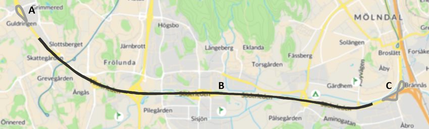
153. Method
Figure 3.1: The route between Fiskebäcksmotet (A) and Åbro-
motet (C) in Gothenburg from the on-road experiment. The light
grey lines represents the interchange segments (A and C) and the
dark grey line between point A and C represents the motorway
segments (B).
The timestamps for the start and end of each segment were found and compiled
in Microsoft Excel for all test subjects and sessions. For some of the experiments,
the amount of collected data exceeded the data storage, which generated a loss of
videos. In most cases, the lost data were recorded by the camera facing the driving
direction. In order to detect the start and stop of segments in these videos, land-
marks from the environment were observed from the intact videos in other angles.
The landmark from the intact videos was then compared to screenshots from cor-
responding angles from experiments with all videos stored. Examples of landmarks
are road signs, buildings, vegetation, and lampposts. The test subjects drove the
car at similar velocities, making it possible to find events on the route by calculating
the time between events in already analysed experiments. The combination of using
landmarks and calculating time differences made it possible to ensure the position
on the route, even without all videos intact. In order to allow further analysis in
the MATLAB software, the timestamps for the starts and ends of each segment
was compiled in an Excel document that was exported to separate text files that
represented both sessions for all test subjects.
3.4 Processing and analysis of EOG signal in MAT-
LAB
To detect the eye blinks in each segment, the EOG signal needed to be analysed and
processed in MATLAB. This was performed with an algorithm that detected each
blink, which also was analysed manually. Some detected blinks needed to be added,
adjusted, or removed manually. The correctly detected blinks were then categorised
after their occurrence with saccadic eye movements and the length of the duration.
3.4.1 Synchronisation of physical data and segments
The first step in the MATLAB software was to synchronise the start and end of the
segments with the physical data obtained from the EOG measurements. This was
163. Method
made by creating an algorithm that generated a time matrix for each test subject and
session containing four columns and 13 rows. The columns represent the start and
stop of each segment relative to the time of the videos and the start and stop relative
to the physical data. The rows represent the 13 segments defined for one session of
the on-road experiment in Dewesoft, of which seven were interchange segments, and
six were motorway segments with three different levels of automation. Table 3.1
describes the index of the segments in the time matrix. There was a delay between
the recording from the physical data and the videos. This delay was taken into
account when calculating the time matrix. The time matrix was then used in a
blink detecting function in MATLAB.
Table 3.1: Presents the order of all 13 segments in the time matrix
for one session of the on-road experiment.
Index of segment Description
1 Interchange (Åbromotet)
2 Motorway (Åbromotet to Fiskebäcksmotet)
3 Interchange (Fiskebäcksmotet)
4 Motorway (Fiskebäcksmote to Åbromotet)
5 Interchange (Åbromotet)
6 Motorway (Åbromotet to Fiskebäcksmotet)
7 Interchange (Fiskebäcksmotet)
8 Motorway (Fiskebäcksmote to Åbromotet)
9 Interchange (Åbromotet)
10 Motorway (Åbromotet to Fiskebäcksmotet)
11 Interchange (Fiskebäcksmotet)
12 Interchange (Åbromotet)
13 Motorway (Åbromotet to Fiskebäcksmotet)
3.4.2 Blink detection algorithm and manual control of blinks
A MATLAB function developed by Volvo Cars was used to detect blinks in the
EOG data. The function’s inputs were the vertical EOG (VEOG) signal, the time
matrix, the index of the test subject and the session, and the index of the road
segment. When the function had detected all blinks based on the criterion of the
algorithm, a window prompted with the VEOG signal visualised. In this window, the
user was allowed to analyse the detected blinks by stepping through each detected
blink, where the onset, offset, maximum, and half amplitudes were marked for the
current blink while the maximum value of the following blink was marked. Figure
3.2 illustrates the prompting window with two detected blinks. The interface of the
prompting window also allowed the user to process the detected blinks by adding
missed blinks, removing falsely detected blinks or adjust the onset and offset of
detected blinks.
173. Method
Figure 3.2: Illustration of two blinks taken from the prompting
window. The onset, offset, half blink amplitude, and maximum
amplitude is marked on the current blink while only the maximum
amplitude is marked on the following blink.
The prompting window enabled a manual correction of the result from the blink
detecting MATLAB function. Each segment for each test subject was carefully
reviewed and compared to the collected video recordings in the manual analysis. If
it was difficult to establish the occurrence of a blink based on the EOG signal in
the prompting window, the video recordings for that test subject was analysed to
determine if it was a blink or not. It was found that the accuracy of the detecting
function was sometimes inadequate. In some cases, maximum points were marked as
blinks, but the videos revealed that there were no eye closures but other movements
of the eye. Figure 3.3 illustrates such a case, where the second marked maximum
point was detected as a blink, but the video revealed that the test subject was
directing the gaze upwards. Therefore, this false positive blink was removed.
183. Method
Figure 3.3: The cross marking the second blink was not an actual
blink, which the video recordings revealed. Therefore, this false
positive blink was removed manually.
In several other cases, the detecting function failed to identify blinks. In the manual
review, these blinks were seen as unmarked maximum points, which was further
inspected in the videos. If the review proved that the detecting function missed
a blink, it was added manually by determining the onset and offset of the blink.
Another error occurring due to the detection function was that the onset and offset
of the blink were misplaced. This error was eliminated manually by adjusting the
length of the blinks by moving the onset and offset mark. Figure 3.4 illustrates such
an error and how the error was corrected.
193. Method
Figure 3.4: The first image illustrates wrongly detected onset of a
blink. The second image shows the result after manual adjustment
of the onset for that blink.
Several factors influenced the appearance and shape of the EOG signal in the
prompting window. From the manual analysis of the detected blinks, it was dis-
covered that speaking, yawning, movement of the upper body, and considerable
head movements generated drifts in the EOG signals baseline position. This ag-
gravated the detection of blinks for the MATLAB function detecting the blinks, as
203. Method
well as the manual analysis. An example of a baseline drift caused by a yawn is
illustrated in Figure 3.5.
Figure 3.5: Illustration of a baseline drift caused by a yawn.
By analysing the EOG signal and comparing it to the recorded videos, it emerged
that the sun also had a substantial impact on blinking behaviour. When the test
subjects were exposed to extreme sunlight, the number of blinks increased distinctly.
In order to eliminate this factor, periods with abnormally frequent blinks due to
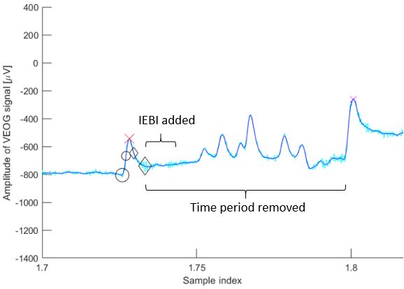
sunlight were removed. Figure 3.6 illustrates a period with an increase of eye blinks
due to extreme sunlight, which was removed from the data. Due to the limitations
of the detecting function, the number of detected blinks were affected by the manual
analysis and processing in some cases. If the baseline drift had a significant effect
on the EOG signal, the detection of blinks was obstructed. In these cases, it was
impossible to ensure that the detected blinks were correct. Therefore, periods where
the baseline drift obstructed the analysis, were also removed to guarantee an accurate
result. This was made by removing blinks that occurred during extreme baseline
drift or sunlight during the manual analysis and processing of the EOG signal.
The removal of blinks caused time periods with incorrectly few blinks, affecting
the blink statistics. To ensure correct blink statistics, the time from the offset of
a correctly detected blink (before the series of removed blinks) to the onset of a
correctly detected blink (after the series of removed blinks) was eliminated. The
eliminated time was replaced with the mean value of the segments inter-eye blink
interval (IEBI). Figure 3.7 shows an example where five blinks are removed due to
extreme sunlight, and the time period between the offset of a correctly detected
213. Method
blink to the onset of a correctly detected blink are removed. The removed time
period is replaced with the calculated IEBI for that segment.
Figure 3.6: An example of an abnormal blinking behaviour due
to exposure to extreme sunlight.
Figure 3.7: Illustration of a removed time period due to abnormal
blinking behaviour caused by extreme sunlight. The removed time
period is replaced with the mean IEBI for that segment.
From the analysis, it emerged that the EOG signal was highly individual among the
223. Method
test subjects, which appeared as differences in duration, amplitude and shape of the
blinks. Hence, the first segments for each new test subject demanded a thorough
comparison between the EOG signal and the recorded videos. This was made to
establish the (individual specific) appearance (duration, amplitude and shape) of
a blink in the EOG signal for a test subject. In some cases, it was challenging to
determine the occurrence of a blink due to vague shapes in the EOG signal. From
the video recordings, it was established that some of these cases emerged due to the
indistinct closure of the eyes during a blink. From the comparison of the VEOG
signal and the video recordings, it also arose that horizontal eye movements were
pronounced in the VEOG signal in some cases. Therefore, it was necessary to in-
vestigate data from each individual electrode to determine if the electrodes were
misplaced. Figure 3.8 illustrates the signals from the separate EOG electrodes.
Judged by the similar shape of the two graphs, vertical movements were obtained
in the electrode that aimed to capture horizontal movements and vice versa. Figure
3.9 also illustrates the EOG signal from separate electrodes but from another test
subject. In this case, the two graphs are different, which means that vertical and
horizontal movements are isolated and captured by the electrodes aimed for that di-
rection. When analysing the vertical EOG signal, blinks are easier detected without
the interference of the horizontal signals. This information highlighted for which
test subjects the detection of eye blinks could be difficult and for whom the manual
analysis and correction was extra important.
Amplitude of VEOG signal [ V]
-2000
-2100
-2200
-2300
-2400
-2500
900 1000 1100 1200 1300 1400 1500 1600 1700 1800 1900 2000
Amplitude of HEOG signal [ V]
-1400
-1500
-1600
-1700
900 1000 1100 1200 1300 1400 1500 1600 1700 1800 1900 2000
Sample index
Figure 3.8: The top figure illustrates the VEOG signal. The
lower figure illustrates the HEOG signal. Their similar appearance
reveals that there was interference between the signals.
233. Method
Amplitude of VEOG signal [ V]
800
600
400
200
0
-200
3000 3500 4000 4500
Amplitude of HEOG signal [ V]
-4100
-4200
-4300
-4400
-4500
-4600
3000 3500 4000 4500
Sample index
Figure 3.9: The top figure illustrates the VEOG signal. The
lower figure illustrates the HEOG signal. There was no interference
between the signals in this case, since the appearance of the signals
are different.
When each segment was analysed and processed manually, the data were saved
in a matrix containing sample index of blink onset (start index), sample index of
blink offset (end index), sample index of blink peak, blink duration (ms), and half
blink duration (ms). The saved data was then used to categorise blinks after their
duration and simultaneous eye movements. For test subject 2, the manual analysis
showed that this individual had an inconsistent blinking behaviour with long eye
closures rather than eye blinks during some segments. Therefore, it was chosen to
exclude the data from this test subject. With test subject 6 excluded as well, the
observations from eight test subjects were used for further analysis.
3.4.3 Categorising blinks into blinks with and without large
saccadic eye movement
After identifying all blinks, the blinks were categorised based on if they occurred
during a large saccadic eye movement or not. A difference in the amplitude of
the EOG signal is an indication of a saccadic eye movement (Ryu et al., 2019).
Therefore, a change in the amplitude of the onset and offset of a blink implied that
the blink occurred during a saccade. An algorithm that detected blinks with and
without large saccadic eye movements based on the VEOG and HEOG signal was
developed in MATLAB. The algorithm calculated the amplitude difference between
onset and offset for each blink for the VEOG signal and the HEOG signal. A
higher and a lower threshold were decided in order to categorise the blinks into
243. Method
three groups. The lower threshold value was 30 µV , and the higher threshold was
60 µV , which correspond to approximately 1.5 and 3 degrees of change in the gaze
angle. The theory regarding the amplitudes of saccades suggests that small saccades
are lower than 5 degrees (Thomas, 1969) and that microsaccades are lower than
approximately 0.5 degrees (Ko et al., 2010). Even during fixation, microsaccades
occur (Ko et al., 2010). Therefore, according to the literature, the threshold for
blinks without saccadic eye movements should have been chosen to 0.5 degrees and
5 degrees as a higher threshold to define larger saccades. These thresholds were
tested in the algorithm and showed that many segments did not contain blinks
agreeing with the thresholds. Therefore, the thresholds were adjusted to 1.5 and 3
degrees, which generated observations in all groups. The thresholds were compared
to the amplitude differences in order to distinguish blinks with and without large
saccadic eye movements. The lower threshold determined the highest amplitude
difference for a blink occurring without a large saccadic eye movement (Group 1),
while the higher threshold determined the lowest amplitude difference for a blink
occurring with a large saccadic eye movement (Group 2). A third category was
introduced to ensure that each category only included blinks with or without large
saccadic eye movements. This category included blinks with an amplitude difference
between the two thresholds and was referred to as the grey zone (Group 3).
3.4.4 Categorising blinks into short, medium, and long du-
ration
The identified blinks were also categorised based on the length of the half blink
duration. The blinks were divided into three categories: short, medium, and long.
A similar grouping of blink duration was performed in a study by Benedetto et al.
(2011). To decide the limits for the categorise, Benedetto et al. used the method of
k-means clustering analysis. Therefore, the limits for the categories were determined
with a k-mean clustering analysis that was performed using the kmeans function in
MATLAB. From this, short blinks were decided to be less than 100 ms, medium
blinks longer than 100 ms but less than 180 ms, and long blinks longer than 180
ms. An algorithm that compared each blink duration towards the decided limits
iteratively was created in MATLAB and generated three new data sets with the
blinks sorted depending on the blink length. The three new data sets were referred
to as Group short (>100 ms), Group medium (100-180 ms), and Group long (You can also read