Smoothing Time Fixed Effects - NO 343 - dice.hhu.de

NO 343

Smoothing Time Fixed Effects

Niklas Gösser
Nima Moshgbar

July 2020

I MP R IN T

DICE DISCUSSION PAPER

Published by:
Heinrich-Heine-University Düsseldorf,
Düsseldorf Institute for Competition Economics (DICE),
Universitätsstraße 1, 40225 Düsseldorf, Germany
www.dice.hhu.de

Editor:
Prof. Dr. Hans-Theo Normann
Düsseldorf Institute for Competition Economics (DICE)
Tel +49 (0) 211-81-15125, E-Mail normann@dice.hhu.de

All rights reserved. Düsseldorf, Germany 2020.

ISSN 2190-9938 (online) / ISBN 978-3-86304-342-1

The working papers published in the series constitute work in
progress circulated to stimulate discussion and critical
comments.
Views expressed represent exclusively the authors’ own
opinions and do not necessarily reflect those of the editor.

 1

Smoothing Time Fixed Effects
 ―PRELIMINARY DRAFT VERSION―

 Niklas Gösser *, # and Nima Moshgbar +, #

 July 2020

 Abstract

 Controlling for time fixed effects in analyses on longitudinal data by means of time-
 dummy variables has long been a standard tool in every applied econometrician’s toolbox.
 In order to obtain unbiased estimates, time fixed effects are typically put forward to
 control for macroeconomic shocks and are (almost) automatically implemented when
 longitudinal data are analyzed. The applied econometrician’s toolbox contains however
 no standard method to control for time fixed effects when time-dummy variables are not
 applicable. A number of empirical applications are crucially concerned with both suffering
 from bias due to omitting time and time-dummies being inapplicable. This paper
 introduces a simple and readily available parametric approach to approximate time fixed
 effects in case time dummy variables are not applicable. Applying Monte Carlo
 simulations, we show that under certain regulatory conditions, trend polynomials
 (smoothing time fixed effects) yield consistent estimates by controlling for time fixed
 effects, also in cases time-dummy variables are inapplicable. As the introduced approach
 implies testing nested hypotheses, a standard testing procedure enables the identification
 of the order of the trend polynomial. Applications that may considerably suffer from bias
 in case time fixed effects are neglected are among others cartel overcharge estimations,
 merger and regulation analyses and analyses of economic and financial crises. These
 applications typically divide time into event and control periods, such that standard time
 dummies may not be applicable due to perfect multicollinearity. In turn, their estimates
 of interest most crucially need to be purged from other (unobserved) time dependent
 factors to be consistent as time may by construction induce omitted-variable bias.

*
 Düsseldorf Institute for Competition Economics (DICE), Heinrich-Heine-University Düsseldorf,
Universitätsstraße 1, 40225 Düsseldorf, Germany.
E-Mail: niklas.goesser@hhu.de.
#
 DICE Consult GmbH, Berliner Allee 48, 40212 Düsseldorf, Germany.
E-Mails: goesser@dice-consult.de; moshgbar@dice-consult.de.
+
 Department of Management, Strategy and Innovation (MSI), KU Leuven,
Naamsestraat 69, 3000 Leuven, Belgium.
E-Mail: nima.moshgbar@kuleuven.be.
 2

1. Introduction

Controlling for time fixed effects in empirical models that are based on longitudinal data has long been
a standard tool in applied empirical applications.1 Time fixed effects allow controlling for underlying
observable and unobservable systematic differences between observed time units. In applied (micro-
) econometric applications, time fixed effects are typically put forward to control for macroeconomic
shocks and are (almost) automatically implemented when longitudinal data are analyzed, in order to
obtain unbiased estimates. Time fixed effects are standardly obtained by means of time-dummy
variables, which control for all time unit-specific effects. This implies controlling for T-1 time-unit
dummy variables in case T time periods are observed in the data. Due to different reasons, in many
applications the observations are measured on a yearly basis, such that time fixed effects are typically
controlled for by T-1 year dummies in case T years are observed in the data.

Time-dummy variables may however be inapplicable in a number of econometric applications due to
perfect multicollinearity. For these applications, the applied econometrician’s toolbox so far contains
no standard method to control for time fixed effects. The lack of controlling for time fixed effects
potentially results in considerably biased estimates, especially in case the variables of interest are
measured conditional on time. This paper introduces a simple and readily available parametric
approach to control for time fixed effects in case time-dummy variables are not applicable. 2

Applications that may especially suffer from bias due to the omission of time fixed effects in the
literature as well as in practitioners’ applications are cartel overcharge estimations, merger and
regulation analyses and analyses of economic and financial crises. In these applications the typical
measurement of events involves dividing time into event and control periods, such that standard time
dummies may not be applicable due to perfect multicollinearity. In turn, their estimates of interest are
constructed conditional on time and thus by construction need to be purged from all time dependent
factors. Time may therefore be regarded as immediate source for omitted-variable bias in these
applications.

Applying Monte Carlo simulations, we show that polynomials of the time trend allow for approximating
time fixed effects which yield consistent estimates under certain regulatory conditions. Our results
show that unbiased estimates can be obtained or at least be approximated under smoothing time fixed

1
 We use the term “longitudinal” in order to indicate that some evolvement over time is present in the data.
Underlying data consistent with our setting can especially be panel data and pooled or repeated cross-sections.
Furthermore, we refer to “time-unit fixed effects” simply as “time fixed effects”.
2
 The suggested parametric approach for obtaining time fixed effects without time-dummy variables can be
expressed as a special case of generalized additive models (GAM).
 3

effects, especially when unobserved time-dependent factors change smoothly over time. In case time-
dummy variables are applicable however, these are clearly superior to smoothing time fixed effects.
Applications in which the event of interest is measured as binary variable conditional on time however,
time-dummy variables are typically not applicable due to perfect multicollinearity, especially when the
event of interest can merely be measured in units of the observable time periods. Our results suggest
that in these cases, time-dummy variables may in turn introduce greater bias if applied.

The empirical literature so far has therefore widely ignored time fixed effects instead, despite a clear
expectation of potential bias in many cases. Smoothing time fixed effects may introduce a crucial albeit
very simple correction in many applications, in which time-dummies would otherwise introduce
additional bias in the estimates. The proposed parametric approach of smoothing time fixed effects
does not make any assumptions about the form or magnitude of the unobserved time-dependent
effects. The order of the trend polynomials however needs to be determined by the user. As the
introduced parametric approach implies testing for nested hypotheses, standard F-tests may guide
determining the order of the trend polynomial that is underlying the data generating process.

Many applications relevant in economic research are concerned with perfect multicollinearity when
time-dummies are included as new regulatory requirements usually start at the beginning of the year
or month and, in general, business decisions are usually made for a full calendar year. Yet, economic
time series are often available merely on the level of the very same time periods. On the one hand
economic time series are usually not available on high frequencies of for example a daily or weekly
basis. On the other hand, many events may not be traced back to a precise starting point, such that
the measurement might be based on an available definition of time merely due to pragmatical
reasons.3

In empirical analyses of economic relations, the underlying time series usually tend to be highly
correlated over time, such that a minimal smoothing requirement is often naturally met. In addition,
time fixed effects also capture all time-unit specific effects, that may be observable or unobservable
or at least unobservable to the researcher.4 The trend variable measuring time can then be included
in the regression equation linearly, quadratically or as higher polynomial approximating the otherwise
discrete steps of time-dummies.5 In turn, with smoothing time fixed effects perfect multicollinearity of
time-dummy variables can be overcome, while retaining the purging properties of time fixed effects.

3
 One example is the financial crisis. It is difficult to define a clear starting point for different industries and
countries.
4
 This may also apply to other field of research such as in social sciences in general. Wherever it is applied and a
period of time is observed, this problem arises.
5
 Similar to time-dummy variables, only T-2 polynomials can be included.
 4

A similar approach introduced by Carter and Signorino (2010) also acknowledge that time-dummies
may not be applicable in cases of binary dependent variable models and thus suggest the inclusion of
polynomial time approximations. Their analysis entails a binary dependent variable in the case of a
survival analysis in political science. As alternatives to parametric trend polynomials, they also propose
semi-parametric modelling using splines. Carter and Signorino (2010) face a similar challenge as
suggested in this paper. Their approach aims at explicitly modelling time within the context of their
binary dependent variable indicating certain events. Against this backdrop, the event measured by the
binary dependent variable cannot be distinguished from the underlying observed time units. Therefore
time-dummy variables are not applicable in their context either. Thus, in this context, their approach
is not concerned with the approximation of unobservable time fixed effects, but rather aims at
explicitly modelling time in order to make statements about the likelihood and duration of an event.
In applied time series econometrics parametric time trends are frequently used and discussed against
the backdrop of potential spurious correlations and within the context of integration and co-
integration of time-series. Here, deterministic time trends are implemented to model observed time
trends and in the context of extrapolation and prediction models (Mills, 2003).

Application implementing linear time trends in the context of cartel overcharge estimations are
Friederiszick and Röller (2010) as well as Hüschelrath et al. (2013). In these papers, the authors
examine the effects of the cement cartel in Germany on cement prices. Implementing a linear trend in
their models, the authors argue that many of the explanatory variables follow a linear time trend and
may thus be more flexibly represented by a deterministic time trend polynomial of order one. Rather
than a leaner data set, as put forward by the authors, the argument that the omitted variables may
likely be highly correlated (macro)economic time series is probably valid. Their linear trend variable
may indeed depict these observable as well as other unobservable developments underlying in the
data.

The introduction of trend polynomials does not constitute an entirely novel approach in the empirical
literature. The contribution of this paper however is the introduction of a parametric approach by
means of trend polynomials as a standard tool for approximating time fixed effects. Thus, we provide
an in-depth analysis of the properties of smoothing time fixed effects. Based on our analysis, we
conclude, that smoothing time fixed effects should be introduced as means for obtaining time fixed
effects when time-dummy variables are not available. Although in some settings, smoothing time fixed
effects may only imperfectly approximate the underlying unobserved time-dependent effects, our
results suggest that neglecting time fixed effects altogether typically results in higher bias.

We show that the polynomials of the time trend yield very similar results to time dummy variables in
their mechanism and represent a smoothing of the discrete steps of time dummy variables. For this
 5

reason, the more flexible standard approach using time dummy variables are superior to the trend
polynomials in the context of continuous treatment variables. If it is not possible to include time
dummy variables due to collinearities, smoothing time fixed effects are a reliable alternative under
certain regulatory conditions.

2. Empirical Setting

The applied econometrician typically does not observe the full set of time-dependent variables
underlying in longitudinal data and thus crucially relies on time fixed effects. The estimation equation
is then of the form:

 = 0 + 1 1 + 2 2 + 

 = 3 3 + 

in which = 3 3 + is the empirical residual and is the error term. Hence, 3 represents an
unobservable omitted variable and thus leads to a bias if the variable of interest 1 is correlated with
 3 . In this setting, 3 only depends on time, such that a standard inclusion of time-dummy variables
may sufficiently represent the underlying unobservable time-effects. The bias may thus be corrected
by means of time-dummy variables in case applicable. The unobserved time-dependent variable 3 
represents numerous unobserved effects in real applications. Time-varying observed or unobserved
effects in (micro-)economic applications are typically assigned to macro-economic developments. The
underlying unobserved time-varying variables will however typically differ depending on the subject
matter.

Smoothness of underlying time series

Many underlying macro-economic time series may be characterized as rather smoothly evolving over
time, once seasonality has been controlled for.6 Smoothness of the underlying unobservable variables
is a favorable property for smoothing time fixed effects. A readily available measure for smoothness is
the lag one autocorrelation Corr( 3 , 3 −1 ). The higher the correlation the smoother is the time
series. Table 1 shows the smoothness of time series from different fields of economic research. These
macro-economic time series show an average smoothness factor of at least 0.61, but typically above

6
 Note that in the typical setting, in which time-dummy variables result in biased estimates, seasonal dummy
variables will still often be applicable. If the data frequency allows, seasonal dummy variables may further
increase smoothness.
 6

0.9. Even the typically very volatile time series for energy prices (here import prices for mineral oil &
electricity price index) show a high smoothness factor.

Table 1: Smoothness of economic time series

 Series Smoothness Min Max Mean Sd Length
 Mineral oil 7 0.607 88.2 183.6 133.95 34.92 15
 GDP8 0.989 75.4 114.8 96.21 11.15 25
 Unemployment9 0.986 3 9.6 5.47 1.71 156
 HCPI10 0.9978 75.7 105.5 89.74 9.64 24
 PPI11 0.9621 83.03 104.18 94.30 7.62 19

Smoothness is characterized by the first lag correlation of the underlying unobserved time-series.

In order to introduce an intuitive approach to smoothing time fixed effects, we first postulate a number
of properties for the unobserved time-dependent variable as well as the variable of interest. Before
we relax these assumptions in the Monte Carlo simulations in section 3, we show results from Monte
Carlo simulations conditional on the form of the curvilinearity of 3 . For the matter of comparison
between time-dummy variables and smoothing time fixed effects, we first show results from Monte
Carlo simulations, in a setting in which both are applicable. Both are applicable in case the variable of
interest is measured continuously. Subsequently we shall concentrate on the setting in which the
variable of interest is merely measured binary, with a strict time division into event and control
periods, where time-dummy variables are inapplicable. The postulated curvilinearity of the underlying
unobservable time-series 3 in this section can entail three different forms. We postulate three
different intuitive forms, a linear time trend, a u-shaped or of a cubic form. Figure 1 shows the
postulated courses.

Data generating process

With a time-range of T = 20 time-units, the data generating process further assumes that is normally
distributed around 0 with a standard deviation of 10. The variable of interest 1 is either simulated
as a continuous (section 2.1) or a binary (section 2.2) variable. The additional explanatory variable 2 
is generated to be exogenous and normally distributed with a mean of 0 and a standard deviation of
10. The true coefficients are postulated as 0 = 10, 1 = 15, 2 = 2 and 3 lying randomly between
10 and 50 for the simulation with a continuous variable of interest 1 (section 2.1) and between 0.5

7
 Statistisches Bundesamt (2020), Index of import prices: GP09-061.
8
 Eurostat (2020), GDP at market prices for the EU28, Index 2010=100.
9
 Statistisches Bundesamt (2020), monthly unemployment rate (ILO-Concept): 13231-0003.
10
 Eurostat (2020), Harmonized Consumer Price Index - Germany – yearly data, Index 2015=100.
11
 OECD (2020), Producer Price Index – EU28 – yearly data, Index 2015=100.
 7

and 1 for the binary variable of interest 1 (section 2.2).12 The dependent variable is then simply the
result of the generated (pseudo-)random variables and the postulated intensities of their effects.

For all simulations, the absolute correlation between the variable of interest 1 and the unobservable
 3 is restricted to [0.3,1). This is done in order to postulate an initial bias if time fixed effects are not
controlled for.13

Figure 1 Figures of three postulated forms of the unobserved time-dependent error

 3 = 100 − 3 = 100 − 3 + 0.1 2

 3 = 100 − 5 + 0.41 2 − 0.01 3

Three postulated forms for the unobserved underlying time-dependent error with the assumed respective underlying
equations. First: linear. Second: quadratic. Third: cubic.

In order to obtain comparisons of approaches, different models are estimated on the basis of the
randomly simulated data. Model 1 is the baseline model neglecting time-varying effects altogether.

12
 Since the relative influence of the error term on y increases drastically in the case of the binary treatment, the
restriction on 3 is conducted.
13
 Note, the correlation may be negative or positive. A correction of bias by means of time fixed effects works
irrespective of the direction of the correlation. A restriction to an absolute correlation therefore suffices.
 8

Model 2 is nested in model 1 and includes T-1 time-dummy variables. Model 3 is nested in model 1
and uses smoothing time fixed effects, polynomials of the time trend with the power p up to P.14

 Modell 1: = 0 + 1 1 + 2 2 + 

 Modell 2: = 0 + 1 1 + 2 2 + ∑ −1
 =2 ∗ + 

 Modell 3: = 0 + 1 1 + 2 2 + ∑ =1 ∗ + 

In the following, the simulations are carried out for a continuous (chapter 2.1) and a binary (chapter
2.2) variable of interest 1 . The respective data generating process of 1 is introduced in the
respective chapter as well as simulation results.

Testing for the optimal order polynomial

As model 3 is nested in the baseline model 1, standard F-tests can be implemented to determine the
optimal order polynomial. As it is readily available, we suggest a testing procedure using a F-tests in
order to detect the optimal order of the polynomial for smoothing time fixed effects. The procedure
entails testing for a sequential addition of trend polynomials starting from a trend polynomial of order
one, as long as the F-statistic rejects the null hypothesis of no explanatory power of the added
polynomial.

As smoothing time fixed effects imply a polynomial approximation of an unknown function and in
practice clear-cut solutions might be rare from this condition alone, we suggest to impose two further
restrictions to the test procedure. First, the additional polynomial should only be included if the t-
statistics of all trend coefficients individually are significantly different from zero as well. If one of these
conditions is not met for the additional polynomial, polynomials up to the last polynomial meeting
both conditions should be used. Second, an exception from this rule should be the first order, linear
polynomial as curvilinear errors must not necessarily follow a linear time trend. The curvilinear error
might rather be stationary or even perfectly stationary. In such a case the first F-test on a merely linear
time trend as well as the individual t-test will of course be insignificantly different from zero. Such a
setting however does not necessarily imply that no curvilinearity is apparent. Therefore, we suggest
that if one or both tests indicate insignificant results, the quadratic polynomial should be tested as
well. In case, both the F-test on the quadratic polynomial is significant as well as the two individual t-

14
 If model 3 is referred to in the following, a parametric regression model with polynomial approximation is
always meant, regardless of the order of the polynomial. The order of the polynomial can range from 1 to T-2.
 9

statistics of linear and quadratic polynomials, the procedure should start from there ignoring the mere
linear trend.15

The testing procedure can be summarized as follows:

 Include time trend polynomials of orders 1 to p in the model. Conduct the F-test for the pth order
 polynomial and t-tests for order polynomials 1 to p. If all tests are significant repeat from the
 beginning, this time with order polynomials 1 to (p+1). The optimal order polynomial is the last
 for which all tests are significantly different from zero.

 The first order polynomial constitutes a special case: if the test procedure at stage 1 results in
 insignificant test-statistics, in any case also test for polynomials 2 to p and follow the above
 procedure.

In the simulations we also conduct this test procedure and report the results from automatically
choosing the indicated optimal order of the polynomial derived from the tests. Results based on the
choice the automatic decision concerning the order of the polynomial from the test procedure are
labelled with the suffix “optimal” in the following sections.

2.1 Continuous Variable of Interest

In this subsection, a setting with a continuous variable of interest is assumed as in this setting both
time-dummy variables and smoothing time fixed effects can be estimated allowing for a comparison
of their respective properties. In practice, time dummy variables are standardly included in the
regression in this setting. The following simulations are conducted three times, one for each of the
three postulated forms of 3 . The continuous variable of interest 1 is generated using the Cholesky
decomposition in order to postulate the desired correlation between and 1 . The generated
random time series thus obtained serves as the basis of the data generating process of 1 . 1 is
generated to be normally distributed around the time series 1 with a standard deviation of 5

 1 ~N( 1 , 5) , [1,20].

The Monte Carlo approach entails the simulation of 1,000 randomly generated data sets with the given
properties. Table 2 shows the 95-%-confidence intervals of the estimated coefficients for each model
and each postulated 3 . An approach is considered consistent if it efficiently yields unbiased
estimates. We consider an approach consistent if the postulated true value of the coefficient lies within

15
 A significance level of = 0.01 for both F- and t-tests was used to conduct the presented simulations.
 10

the 95-% confidence interval of the empirical distribution of estimated coefficients, based on
estimating from a sufficiently large number of randomly generated data sets.

Table 2: 95-% Confidence intervals for the postulated shapes and each model

 Postulated true form of error
 (1) (2) (3)
 Estimated model Linear 3 U-Shaped 3 Cubic 3 
 Model 1 – none (20.2872; 20.6616) (20.3189; 20.6995) (18.2042; 18.4316)
 Model 2 – dummy (14.9990; 15.0022) (14.9980; 15.0009) (14.9991; 15.0021)
 Model 3 – linear (14.9995; 15.0009) (16.3376; 16.5429) (17.6132; 17.8166)
 Model 3 – squared (14.9995; 15.0010) (14.9991; 15.0005) (15.5565; 15.6604)
 Model 3 – cubic (14.9995; 15.0010) (14.9990; 15.0005) (14.9995; 15.0009)
 Model 3 – optimal (14.9995; 15.0010) (14.9991; 15.0005) (14.9996; 15.0009)

Continuous variable of interest: 95-% Confidence intervals of the empirical distribution of 1, the estimated coefficient for 1 ,
from a Monte Carlo simulation entailing 1,000 randomly generated data sets.

In Table 2 the confidence intervals of the respective models indicated in column 1 are shown. The true
postulated coefficient is 1 = 15. The postulated shape of the error introduced in Figure 1 is indicated
in row two of Table 2. The underlying true shape of the error in column (1) is linear, in column (2) the
true curvilinear shape of the error is u-shaped and in column (3) the postulated true shape is cubic.
The rows show results of each testing procedure. As introduced above, model 1 ignores time fixed
effects altogether and model 2 controls for time fixed effects by means of dummy variables. Model 3
controls for time fixed effects using smoothing time fixed effects and is estimated with four different
approaches. The three first specifications include only a linear trend (“model 3 – linear”), a linear and
a quadratic trend (“model3 – squared”), a linear as well as a quadratic and a cubic trend (“model3 –
cubic”). The last row shows results from the automatically chosen order of the polynomial based on
the test procedure described above (“model3 – optimal”).

As bias postulated in the empirical specifications throughout, model 1, in which time fixed effects are
neglected altogether is biased disregarding the curvilinear form in the error. As time dummy variables
are applicable when the variable of interest is continuous, model 2 is unbiased throughout. In the
simple case with a postulated linear error as in columns (1), smoothing time fixed effects of order 1 is
unbiased. The order polynomial of up to 3 remains unbiased. In case of postulated quadratic errors,
unbiased estimates are obtained as of a quadratic trend polynomial. Similarly, in case of postulated
cubic errors, the Monte Carlo simulations result in unbiased estimates as of a polynomial of order 3.
Model 3 with automatically chosen order of the implemented polynomials based on the test procedure
above yields consistent estimates.

 11

The Monte Carlo simulations show that both time dummy variables as well as smoothing time fixed
effects with the right order polynomial result in unbiased estimates. Smoothing time fixed effects yield
consistent estimates and show to be reliable in case implemented correctly. Since the setting allows
time dummy variables, these are however clearly favorable as they are not only consistent, but also
more flexible and its implementation needs virtually no specific attention.

2.2 Binary Variable of Interest

In case the variable of interest is binary time-dummy variables are inapplicable. The binary variable of
interest 1 takes on a binary form

 1 ≤ 10
 1 = {
 0 > 10

Although the setting is based on cartel overcharge estimations, the general results hold for other cases
in which the variable of interest indicates events based on time. In this setting the variable of interest
 1 now splits the dataset in half. Correlations between 1 and the unobserved 3 will almost
automatically arise since 1 is immediately based on time and 3 is likely to change over time. Since
the relative effect of 1 ∗ 1 on compared to the relative effect of 3 ∗ 3 on is now much
smaller compared to the continuous case, 3 is restricted to values between 0.5 and 1. 16 Again, the
simulation was conducted using 1,000 repetitions.

As bias postulated in the empirical specifications throughout, model 1, in which time fixed effects are
neglected altogether. As time dummy variables are not applicable when the variable of interest is
discrete and indistinguishable from time-units, model 2 is biased throughout. In the simple case with
a postulated linear error as in columns (1), smoothing time fixed effects of order 1 is unbiased. The
order polynomial of up to 3 remains unbiased. In case of postulated quadratic errors, unbiased
estimates are obtained as of a linear trend polynomial already. Due to the postulated rather flat u-
shape in the simulation, a linear approximation of underlying time-dependent effects suffices to obtain
unbiased estimates. In case of postulated cubic errors, the Monte Carlo simulations result in unbiased
estimates as of a polynomial of order 3. Model 3 with automatically chosen order of the implemented
polynomials based on the test procedure above yields consistent estimates throughout on average.

16
 Before, the continuous 1 had a mean of 100. Now it takes on the value 1 or 0. Hence, the relative effect of
the error term containing 3 ∗ 3 on the variance of would be much higher now and the resulting bias
would therefore be extremely high. Therefore, the restriction on 3 ensures comparability.
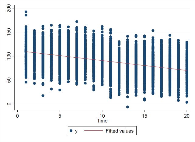
 12

Table 3: 95-% Confidence intervals for the postulated shapes and each model

 Postulated true form of error
 (1) (2) (3)
 Estimated model Linear 3 U-Shaped 3 Cubic 3 
 Model 1 – none (22.4321; 22.6174) (21.6925; 21.8646) (16.8100; 16.8665)
 Model 2 – dummy (29.1247; 29.4824) (27.7121; 28.0374) (23.4334; 23.6579)
 Model 3 – linear (14.9627; 15.0251) (14.9441; 15.0394) (12.1302; 12.2429)
 Model 3 – squared (14.9626; 15.0250) (14.9626; 15.0250) (11.9095; 12.0074)
 Model 3 – cubic (14.9583; 15.0396) (14.9583; 15.0386) (14.9871; 15.0701)
 Model 3 – optimal (14.9624; 15.0248) (14.9651; 15.0280) (14.9869; 15.0699)

Binary variable of interest: 95-% Confidence intervals of the empirical distribution of 1, the estimated coefficient for 1 , from
a Monte Carlo simulation entailing 1,000 randomly generated data sets.

The Monte Carlo simulations show that time dummy variables are inconsistent in case the variable of
interest is binary. Smoothing time fixed effects with the correct order polynomial reliably result in
unbiased estimates in case implemented correctly. Implementing time dummy variables in such a
setting is at least as harmful as neglecting time fixed effects altogether as is commonly done in the
literature.

2.3 Graphical Analysis

For determining the order of the polynomial, a graphical analysis could be regarded as obvious
approach since the dependent variable could in some cases already show a certain curvilinear form
indicating a suitable order of the polynomial. Although this might be the case in some applications, a
well-grounded economic analysis as well as a highly careful analysis of the empirical properties are
inevitable.

In this section we show that often a graphical analysis of the curvilinearity of the dependent variable
as well as the multivariate fitted residuals can give first insight about whether or not to include
smoothing polynomials, and an indication of the order of the polynomial.

Figure 2 shows an example of the data generating process from section 2.2. The left hand panel shows
the scatter plot for the dependent variable . The scatter plot depicts the postulated linear time trend
of the unobserved variable 3 clearly in the dependent variable. Even the corresponding residuals
plotted on the right panel show the linear trend. In this case, the scatter plots can give a good indication
for an unobserved linear time series that will bias the binary variable of interest.

 13

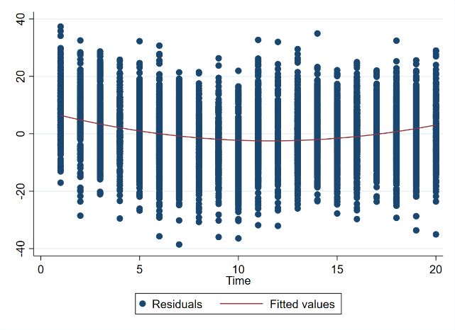
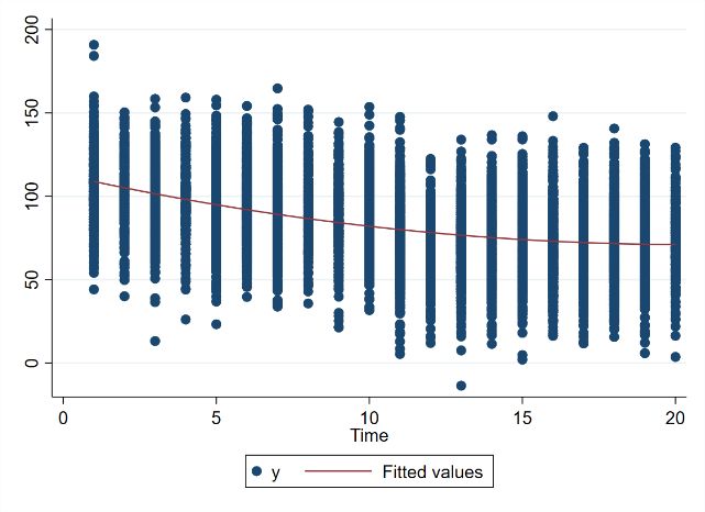
Figure 2: Linear error: Scatter plots

Linear error, binary variable of interest. Left panel shows scatter plot of dependent variable over time as well as bivariate
regression line. Right hand panel shows fitted empirical residuals from a specification neglecting time fixed effects. Linear
error graphically clearly visible.

The example depicted in Figure 3 comes from the data generating process with postulated u-shaped
 3 . Again, the scatter plot of against time shows the postulated u-shaped 3 . The same is true for
the scatter plot of the residuals from the model 1 neglecting time fixed effects.

However, in both cases the second graph might be misleading. While the scatter plot of clearly
indicates systematic differences over time, an analysis of the respective right panel scatter might guide
the conclusion that there are no systematic time dependent differences. On the contrary, in both cases
the OLS regression per construction attributes the unobserved time differences to the variable of
interest.

However, analyzing the two scatter plots of a given specification can on the one hand give an indication
on whether or not smoothing polynomials might be appropriate and on the other hand they can give
first insights on an appropriate order of the underlying polynomial.

A sole graphical analysis is however by no means sufficient as such graphical analyses may not always
give a clear indication as in the rather clear examples shown. In real world applications, a clear visually
derivable potential curvilinear form is probably rare. In other words, solely relying on a graphical
absence of clear (curvilinear) of systematic changes over time may considerably misguide in choosing
a suitable specification.

 14

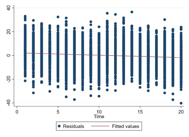
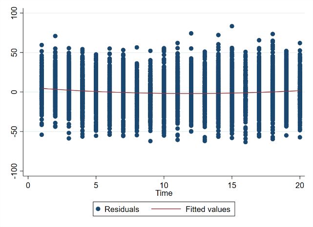
Figure 3: Quadratic error. Scatter plots

Quadratic error, binary variable of interest. Left panel shows scatter plot of dependent variable over time as well as bivariate
regression line. Right hand panel shows fitted empirical residuals from a specification neglecting time fixed effects. U-shape
graphically clearly visible.

Figure 4 again shows scatter plots for and the residuals from model 1. The data generating process
from chapter 2.2 has been modified for this example. First, an additional observable variable 4 has
been included. This variable is a random variable that is normally distributed around 3 with a
standard deviation of 10. The respective coefficient 4 however equals −1 ∗ 3 . In addition, the true
error term now has a standard deviation of 20 instead of 10. This setting yields to a severely biased
coefficient of 1 = 21.86. However, due to the additional explanatory variable 4 and an increased
influence of , the scatter plots in Figure 4 cannot give any clear indication on whether or not to
include smoothing polynomials and also not on the appropriate order of a polynomial. From the first
scatter plot it can be seen that one might come to the conclusion that the unobserved variable might
take on an inverted u-shape. The scatter plot of the multivariate residuals however, might give a hint
on the u-shaped 3 . By and large, the scatter plots almost indicate a linear relationship.

Nevertheless, graphical analyses should always be the first step in exploring for a model specification.
As the minimal-examples however show, merely relying on a graphical inference is of course
insufficient and may considerably misguide in real applications. Graphical analyses should always be
crucially accompanied by economic rationale and formal testing. 17

17
 The testing procedure suggests implementing a quadratic polynomial, which is the true postulated curvilinearity in the
 ̂1 = 15.47 with a given true parameter 1 = 15.
error, and leads to an estimate of 
 15

Figure 4: Quadratic error: Scatter plots

Quadratic error, binary variable of interest. Left panel shows scatter plot of dependent variable over time as well as bivariate
regression line. Right hand panel shows fitted empirical residuals from a specification neglecting time fixed effects. Postulated
u-shape graphically almost flat.

3 Monte Carlo Simulations

In this section, results from more in-depth Monte Carlo simulations are shown. For this purpose, a
modified data generating process compared to chapter 2 is used. The assumption of a clear curvilinear
form of 3 is now relaxed, such that the unobserved variable is generated randomly.

Although the main focus is on a binary variable of interest, the setting with a continuous variable of
interest is addressed again as well. For the simulation in the setting with a continuous variable of
interest, the Cholesky decomposition is crucial. The data generating process is in line with chapter 2.1.
Nevertheless, in this case instead of postulating the curvilinear form of 3 , both, 1 and 3 are
generated by a Cholesky decomposition. Again, the mean of both, the variable of interest and the
mean of 3 equals 100 and the standard deviations are equal to 20. Again, the correlation is set to
vary between 0.3 and 1. 18 The simulated data sets cover 10 time periods. As before, all regression
models are estimated using OLS.

In this standard setting the traditional time dummies are superior compared to the smoothing
polynomials. Even though, the latter can also overcome the bias like already seen in chapter 2, the
dispersion of estimated coefficients now is significantly larger. The mean squared error (MSE) for

18
 This is true for both the correlation between the underlying time series generated by the Cholesky
decomposition and the actual correlation between 1 and 3 . The latter might differ, since 1 is generated to
be distributed around an underlying time series generated by the Cholesky decomposition. The smoothness is
restricted to values of at least 0.6.
 16

model 1 equals 422.13, the MSE for model 3 using smoothing time fixed effects with polynomials of
optimal order equals 52.54 and for model 2 with the time dummies the MSE is 0.001.19 This shows that
even though a very large bias has been imposed by construction within the underlying simulation, the
time dummies are not only unbiased but also efficient. Therefore, the time dummies are rightfully the
standard tool of every econometrician for these kinds of settings. Since this is already well known our
contribution to the literature is the use of smoothing time fixed effects in case time dummy variables
are not available, only the latter setting will be discussed in more depth in this chapter.

Hence, a Monte Carlo simulation with binary variable of interest is carried out. The data generating
process is closely linked to the data generating process in chapter 2.2. Time-series 3 is generated in
line with chapter 2.1 and has a mean of 100 and a standard deviation of 20. Variable 1 takes on the
following binary form:

 1 ≤ 5
 1 = {
 0 > 5

The resulting data set spans over 10 time periods. In line with the simulation in chapter 2.2 , 3 is
restricted to only vary between 0.5 and 1. Also, the correlation between the variable of interest 1 
and the unobservable 3 is restricted to [0.3,1) in order to constitute bias by construction. The true
coefficients 0 = 10, 1 = 15 and 2 = 2 stay the same, so do 2 and .

In the following, imposed restrictions on the Monte Carlo simulations will be gradually relaxed in order
to analyze performance properties of smoothing time fixed effects. Our results show that the
smoothness of the unobserved time series 3 and the correlation between 1 and 3 play a
considerable role in the performance of the smoothing time fixed effects.

Typically, economic time series are highly smooth over time. For the following analysis, the
smoothness is measured by the lag-one autocorrelation:

 Corr( 3 , 3 −1 ).

There are other measurements for smoothness, but the lag-one autocorrelation has the advantage
that it allows easy statistical interpretation. A correlation close to one implies a smoothly varying time
series, while a score around 0 implies that there is no overall linear relationship between one
observation and the following. A score close to -1 on the other hand implies that the series regularly
jumps around the mean in a very particular way. If one observation lies below the mean, the next one
is likely to be above the mean by approximately the same amount.

19
 The simulation has been conducted using 1,000 repetitions.
 17

Smoothing time fixed effects under realistic regulatory conditions

Table 1 from section 2 shows different time series from different fields of economic research. It can be
seen that the time series have on average a very high smoothness factor of more than 0.9 which also
shows that typically no disruptive shocks occur. In order to analyze the properties of smoothing time
fixed effects in a typical realistic setting, the Monte Carlo simulations are restricted such that the lag-
one autocorrelation of the unobserved time series is larger than 0.7. Furthermore, extreme
correlations between 1 and 3 larger than 0.9 are ignored. The results are summarized in Table 4.

Table 4:Results from Monte Carlo simulation with a realistic setting
 Mean Sd MSE
 Model 1 – none 24.39 24.89 24.64 6.77 138.83
 Model 2 – dummy 29.66 30.57 30.11 12.34 380.60
 Model 3 – opt 14.82 15.33 15.08 6.97 48.64
 Model 3 – min 14.84 15.06 14.95 3.02 9.15

Results from 2,839 data sets from the Monte Carlo simulation that are left after imposing the restrictions ( 3 , 3 −1 ) >
0.7 and ( 1 , 3 ) ∈ (0.3,0.9). 95-% Confidence intervals are shown. shows the lower bound and reports the
upper bound of the confidence interval.

It is obvious from the results that the bias of model 1 is severe since the regressions do not control for
unobserved time changes altogether. The mean of the estimated coefficients is biased by 9.64. Due to
the very setting with a discrete variable of interest, time dummy variables in model 2 cannot solve the
bias due to perfect multicollinearity. The bias even increases under model 2. Smoothing time fixed
effects yield unbiased estimates (model3 – opt). Their confidence intervals include the true coefficient,
which takes the value 15. Here, “model 3 – opt” refers to the model for which the order of the
polynomial has been chosen using the suggested testing procedure from chapter 2. “Model 3 – min”
on the other hand refers to the theoretically perfect model, in which the polynomial has been chosen
such that the bias of the estimated coefficient is minimal.20 This of course is just a theoretical approach,
but it allows to examine the performance of the smoothing time fixed effects separated from the
performance of the suggested test. Table 4 shows that the suggested testing procedure yields unbiased
estimates within this setting. Nevertheless, compared to “model 3 – min”, the standard error and hence
the MSE are significantly higher.

20
 Unlike in a Monte Carlo simulation, in real applications the latter is of course never observable since the true
parameter is unknown to the researcher.
 18

Table 5: Results from Monte Carlo simulation with a realistic setting II

 Mean Sd MSE
 Model 1 24.96 26.13 25.55 7.20 163.03
 Model 2 31.42 33.44 32.34 12.48 459.38
 Model 3 - opt 14.72 15.72 15.22 6.16 37.93
 Model 3 - min 14.69 15.12 14.90 2.67 7.11
Results from 584 data sets from the Monte Carlo simulation that are left after imposing the restrictions ( 3 , 3 −1 ) >
0.8 .

Table 5 shows another realistic setting in which the restrictions regarding the correlation between 1 
and 3 is relaxed but the ssmoothness of 3 is set to be higher than 0.8. Again, both “model 3 – min”
and “model 3 – opt” deliver unbiased estimates. Due to the higher smoothness in turn, the dispersion
of the estimated coefficients decreases.

Relaxing restrictions on smoothness

In order to further analyze the properties of smoothing time fixed effects, the so far imposed
restrictions regarding the smoothness of 3 are relaxed. The simulation now allows the smoothness
parameter to vary between -1 and 1.21 Table 6 shows descriptive statistics for different smoothness
values.

Table 6: Estimates depending on the smoothness of 3 

 Smoothness (-1,0] (0,0.2] (0.2,0.4] (0.4,0.6] (0.6,0.8]
 N 48,894 24,168 17,343 7,762 1,671
 ( 1 , 3 ) 0.43 0.48 0.52 0.59 0.66
 Model 1- none Mean 20.96 21.64 22.18 23.10 24.15
 Sd 4.40 4.99 5.45 6.18 6.66
 Model 3 – opt Mean 23.66 20.50 18.71 17.03 15.95
 Sd 16.38 15.28 13.67 11.85 9.06
 Model 3– min Mean 19.21 17.57 16.65 15.90 15.33
 Sd 8.34 7.63 6.52 5.30 3.94

Results from a Monte Carlo simulation with 100,000 randomly generated data sets and the restriction ( 1 , 3 ) > 0.3.
We refrain from showing results from time dummy variables as they are extremely biased and thus can be regarded as
inapplicable due to the underlying setting.

21
 The correlation between 1 and 3 is still restricted to only vary between 0.3 and 0.9.
 19

From Table 6 follows that the performance of smoothing time fixed effects crucially depends on the
smoothness of the unobserved time series. Both specifications of model 3 result in less bias and less
variance of the estimated coefficients the larger the smoothness parameter. Both smoothing time
fixed effects with optimal order polynomial as well as minimal bias approximate the true parameter
 1 = 15 increasingly well the smoother the underlying bias becomes. In line with Table 4 both the
expected value and the standard deviation for the models with tested order of polynomials is strictly
larger compared to the model with minimal bias.22

Furthermore, the correlation between 1 and 3 per construction increases if the smoothness of the
unobserved time series 3 increases. Since 1 is a binary variable based on time, a smoother 3 will
yield a larger correlation. In order to obtain an initial bias in the first place, all cases in which 3 does
not or only changes slightly over time are eliminated. However, due to increased smoothness, bias
correcting properties of smoothing time fixed effects overweigh the additional initial bias stemming
from increased correlation.

Relaxing restrictions on correlations

Regarding correlations, so far only the correlation between 1 and 3 have been shown. However,
correlations between the unobserved variable 3 and the dependent variable 1 as well as also
play a crucial role for unbiased estimations of 1 . Table 7 gives an overview of the means of the
estimated coefficient for different combinations of correlations Corr( 1 , 3 ) and Corr( , 3 ).
With regard to the correlation between 1 and 3 it can be seen that a small correlation typically
results in an overcorrection of the otherwise overestimation due to omitted variables bias that would
arise from model 1, within a certain range of values for Corr( , 3 ).23 A high correlation between
 1 and 3 on the other hand results in downwards corrected coefficients compared to model 1, still
entailing a positive bias of the estimated coefficients. These two effects overlap each other. While a
higher correlation leads to a higher omitted variables bias, which has to be overcome by time fixed
effects, for a low correlation between 1 and 3 the bias is less pronounced and hence smoothing
time fixed effects consume too much of the variance of . Hence the effect of 1 is underestimated
and the original bias overcorrected. The correlation between 1 and 3 on the other hand does not
influence the direction but rather the intensity of the bias. For higher degrees of smoothness, for

22
 For either model, the confidence interval never includes the true coefficient 1 = 15. For the last column, the
CI for the model with tested order of the polynomial approximation equals [15.51,16.38] and for the optimal
polynomial [15.14,15.52].
23
 Model 1 estimates a ̂1 = 23.46 for which both correlations are in the range of [0.3,0.65).
 20

example at least of 0.8, all results shown in Table 7 will improve overall.

Table 7: Mean and standard deviation of estimated coefficients depending on ( 1 , 3 ) and ( , 3 ).

 Corr( , 3 )
 [0.3,0.65) [0.65,1] [0,1]
 [0.3,0.65) 14.13 12.91 14.24
 (4.00) (9.71) (3.91)
 [0.65,1] 16.07 17.90 16.11
 Corr( 1 , 3 )
 (3.46) (8.17) (3.95)
 Overall: [0.3,1] 15.42 16.69 15.40
 (3.76) (8.82) (4.04)

Monte Carlo simulation with 10,000 randomly generated data sets. Standard deviation in parentheses. Restriction to
smoothness ( 3 , 3 −1 ) > 0.6. True parameter is 1 = 15.

4. Discussion

In this section we discuss the simulation results as well as the test procedure and implications of
smoothing time fixed effects. Furthermore, we address selected related topics in the given context.

Results from the Monte Carlo simulation

Table 8 summarizes the results from the Monte Carlo simulations. For different combinations of
correlations, the bounds of the confidence intervals of the estimated coefficients are shown, as well
as the frequency of the randomly generated data sets left after imposing the respective restrictions.
In addition, the results are presented separated by degrees of smoothness. Again, “Model 3 – opt”
refers to the smoothing time fixed effects following the suggested testing procedure. “Model 3 – min”
refers to the model where the order of the polynomial is chosen in terms of minimal error between
the estimated and the true coefficient.

It can be seen that smoothing time fixed effects can best approximate smooth changes in the
unobserved variables. However, erratic changes and extreme shocks can be correctly controlled for up
to a certain extent. A higher degree of smoothness leads to overall unbiased estimates, while a lower
degree of smoothness can only partly correct the bias. For the simulations with a smoothness of the
unobserved variable 3 that is larger than 0.8, only the estimated coefficients for simulated data sets
with both Corr( , 3 ) and Corr( 1 , 3 ) smaller 0.65 but higher 0.3 are biased (see Table 8). In
addition, the estimates for Corr( , 3 ) > 0.65 and small Corr( 1 , 3 ) are only somewhat
 21

reliable, since only 4 simulated data sets remain after imposing the restriction. All in all, the
smoothness of the unobservable 3 has a positive effect on the estimations using smoothing time
fixed effects. Both, the overall bias and the dispersion of the estimated coefficients significantly
decrease.

With regard to the correlation between and 3 it can be seen that a higher correlation will enlarge
the overall bias. This is very intuitive since this corresponds to a higher influence of the error term on
the variance of . The larger the influence, the larger the omitted variables bias will be.

While the smoothness of 3 and the correlation between and 3 only impact the magnitude of
the bias, the correlation between 1 and 3 on the other hand influences the direction of the bias.
For small values of Corr( 1 , 3 ) the model with smoothing time fixed effects leads to an
overcorrection of the initial bias. For large values of Corr( 1 , 3 ) the initial omitted variable bias
from model 1 becomes very high.24 In this case, smoothing time fixed effects cannot fully correct the
bias, such that a portion of the bias remains. Therefore, there is a trade-off. Two opposing forces that
are related to the correlation between 1 and 3 influence the direction of the remaining bias. While
a higher correlation enlarges the initial bias that smoothing time fixed effects have to correct, small
values of Corr( 1 , 3 ) might lead to some kind of overfitting. The initially already relatively small
bias will be typically approximated by multiple trend polynomial variables within the regression. These
polynomials might lead to an overfit, that absorb more of the variation of than optimal. In this case,
part of the effect of the variable of interested is absorbed by the approximation. This problem is more
pronounced if the smoothness parameter of 3 is small. In this case, the polynomial approximation
using smoothing time fixed effects is more difficult to achieve compared to an approximation of a very
smooth 3 .

Table 8: Summary of Monte Carlo findings.
 Smoothness>0.6 Smoothness>0.8
 ( , ) ( , ) Model 3 - opt Model 3 - min N Model 3 - opt Model 3 - min N
 0.65 (17.73;18.14) (15.98;16.17) 5,013 (15.08;16.13) (14.83;15.31) 402
 0.65 (20.05;23.06) (17.19;18.60) 514 (13.23;21.38) (13.46;16.57) 43

Summary of the results from the Monte Carlo simulations on smoothing time fixed effects.95-% confidence intervals for several
combinations of ranges for correlations as well as smoothness parameters are shown.

24
 For model 2, there is a clear positive relationship between Corr( 1 , 3 ) and the bias. If Corr( 1 , 3 ) > 0
the bias will be strictly larger than 0. The higher Corr( 1 , 3 ), the larger the positive bias.
 22

Regarding the suggested testing procedure, the results from both chapter 2 and 3 show, that the
resulting regression is unbiased under certain regulatory conditions. However, chapter 3 also
introduces “model 3-min” in which the order of the polynomials has been chosen to minimize the
resulting bias (which in real application are unknown to the researcher). It can be seen that the testing
procedure is not optimal in all ranges of possible values for smoothness and correlations, yet. While
the bias for this model is rather small as well, the dispersion is rather high compared to “model 3-min”.
However, as seen in Table 4 from chapter 2 the testing procedure leads to unbiased estimates for
realistic settings.

Related topics

As the binary variable of interest divides time in two periods of event and control, systematic
differences over time are likely to occur, potentially accompanied by a considerable correlation with
the error term. Hence a bias due to the omission of time fixed effects is very likely to be present from
the very setting. Against this backdrop, autocorrelated error terms extensively discussed in time series
econometrics appear as closely related. If there are systematic differences between event and control
periods, the error terms are likely to be autocorrelated. Hence, autocorrelation of the error terms tend
to signal the presence of bias a bias that are likely to be solvable by time fixed effects.

In this context we would like to refer to the literature on autocorrelation (serial correlation),
stationarity, (co-)integration and spurious correlations. These phenomena are extensively addressed
in time series econometrics. We show that these problems can be related to the problem of an omitted
variables bias in the given setting. The phenomenon of spurious correlations is typically introduced in
a similar way as it is presented in this paper and can be described as a special case in which the true
 1 equals 0. The omitted variable is a confounding factor that is common for both time series. The
omitted variable is therefore serially correlated over time. Nevertheless, since smoothing time fixed
effects can constitute a crucial remedy for unobserved time dependent changes of the error term.

Lastly, we would like to discuss further frequent estimation techniques within similar contexts. In a
setting entailing omitted variable bias, especially instrumental variable regressions are put forwards
when dealing with the present endogeneity. In the given setting however, traditional instruments may
usually not be applicable however, if at all, since an instrument has to meet both validity and
relevance.25 A valid instrument in turn has to depict the time changes of the variable of interest. This

25
 A valid instrument has to meet two conditions. First, it has to be correlated with the variable of interest, hence
be relevant. Second, it has to be uncorrelated to the omitted variable, hence be exogenous.
 23

however may imply that a potential instrument is not exogenous since it may still be correlated to
unobservable variables in the error term. Against this backdrop, the relevance of smoothing time fixed
effects becomes even more pronounced, especially since smoothing time fixed effects themselves do
not introduce additional bias.
The easy and readily available implementation of parametrically modelled smoothing time fixed
effects makes the suggested procedure highly appealing. Since it is applicable for parametric models
estimated by OLS, it is easier and more straightforward to implement compared to potential
alternative approaches such as semi-parametric estimators.

5. Conclusion

For longitudinal data time dummies are the standard method to control for unobserved time
depending effects. However, if the variable of interest depends on time and takes on a binary form,
these are typically no longer applicable due to multicollinearity issues.

Although in this setting, the variable of interest is likely to be biased, the literature typically ignores
the bias altogether, potentially due to a lack of a consistent approach to control for time fixed effects
in this context. Our paper contributes to the literature as we introduce a simple and readily available
parametric approach to control for time fixed effects in case time dummy variables are typically
inapplicable. Although in some settings, smoothing time fixed effects may only imperfectly
approximate the underlying unobserved time-dependent effects, our results suggest that neglecting
time fixed effects altogether typically results in higher bias.

We show that smoothing time fixed effects can mitigate and under certain regulatory conditions even
eliminate the bias caused by omitted variables in this setting. The smoother the unobserved variable
is, the less biased and dispersed the estimated coefficients are. We have shown that economic time
series typically smoothly evolve over time. Under this assumption, we show that under smoothing time
fixed effects unbiased estimates can be obtained. As the introduced approach implies testing nested
hypotheses, a standard testing procedure enables the identification of the order of the trend
polynomial. We show that this procedure works well under certain regulatory conditions, that we
consider as highly realistic.

 24