Probabilistic Modeling of Hurricane Wind-Induced Damage in Infrastructure Systems - Derek Chang, Kerry Emanuel, and Saurabh Amin Massachusetts ...
←
→
Page content transcription
If your browser does not render page correctly, please read the page content below
Probabilistic Modeling of Hurricane Wind-Induced Damage in

                                                              Infrastructure Systems
arXiv:2105.03497v1 [stat.AP] 7 May 2021

                                                       Derek Chang, Kerry Emanuel, and Saurabh Amin

                                                           Massachusetts Institute of Technology

                                                                             1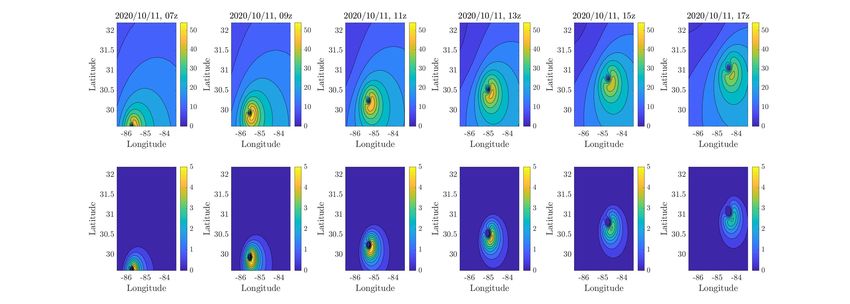
Abstract

          This paper presents a modeling approach for probabilistic estimation of hurricane wind-induced damage to in-

      frastructural assets. In our approach, we employ a Nonhomogeneous Poisson Process (NHPP) model for estimating

      spatially-varying probability distributions of damage as a function of hurricane wind field velocities. Specifically,

      we consider a physically-based, quadratic NHPP model for failures of overhead assets in electricity distribution

      systems. The wind field velocities are provided by Forecasts of Hurricanes using Large-Ensemble Outputs (FHLO),

      a framework for generating probabilistic hurricane forecasts. We use FHLO in conjunction with the NHPP model,

      such that the hurricane forecast uncertainties represented by FHLO are accounted for in estimating the probability

      distributions of damage. Furthermore, we evaluate the spatial variability and extent of hurricane damage under key

      wind field parameters (intensity, size, and asymmetries). By applying our approach to prediction of power outages

      (loss-of-service) in northwestern Florida due to Hurricane Michael (2018), we demonstrate a statistically significant

      relationship between outage rate and failure rate. Finally, we formulate parametric models that relate total damage

      and financial losses to the hurricane parameters of intensity and size. Overall, this paper’s findings suggest that our

      approach is well-suited to jointly account for spatial variability and forecast uncertainty in the damage estimates,

      and is readily applicable to prediction of system loss-of-service due to the damage.

   Keywords: Hurricane Wind Risk, Infrastructural Damage, Probabilistic Modeling, Poisson Process, Outage Pre-

diction

                                                                2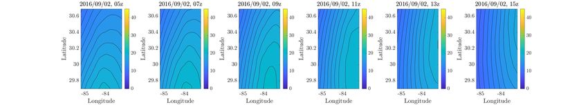
1    INTRODUCTION

Hurricanes are becoming an increasingly critical threat to infrastructure systems, especially as the destructive poten-

tial of hurricanes is expected to increase due to global warming (Emanuel, 2005). Climate simulations of hurricanes

indicate that if little is done to curb greenhouse gas emissions and the world warms by 3-4˝ C this century, then

hurricane rainfall will increase up to a third while wind intensity will be boosted by as much as 25 knots (Patricola

& Wehner, 2018). The deleterious effects of hurricanes on infrastructure systems were highlighted in 2017 when

electric power utilities struggled to handle the aftermath of Hurricanes Harvey, Irma, and Maria. Infrastructural vul-

nerability to hurricanes is further heightened by aging of critical infrastructure assets, as well as increasing coastal

populations and development.

    Effective post-hurricane infrastructure response and recovery strategies require accurate estimation of risk, or

expected cost incurred due to hurricane-induced damage to the infrastructure. Broadly speaking, one computes risk

by integrating the cost associated with infrastructural loss-of-service induced by various damage scenarios, over

the probabilities of these scenarios. Generalized linear or additive regression models are commonly used to predict

outages (i.e., loss-of-service) (Liu, Davidson, Rosowsky, & Stedinger, 2005; Liu, Davidson, & Apanasovich, 2007; Han

et al., 2009) in electric power infrastructure, as a function of parameters related to the hurricane’s physical structure

and the local environment. However, these models do not generate probabilistic, spatially-varying predictions of

damage to infrastructure assets. A lack of adequate damage predictions impedes pre-storm resource allocation,

warehouse selection, vehicle fleet routing, damage localization, and repair operations (Van Hentenryck, Bent, &

Coffrin, 2010; Lee, Dahan, Weinert, & Amin, 2019). Slow damage localization and repair result in an increased time

duration during which the infrastructure fails to adequately provide service to end-users.

    In this article, we focus on modeling of hurricane wind-induced damage to overhead infrastructural assets. The

damages are dependent on hurricane wind characteristics such as local wind speed, direction, and duration, which

are functions of the hurricane track and intensity. The hurricane track forecast is typically provided by the National

Hurricane Center (NHC) hour/days ahead of the hurricane’s forecasted landfall. Forecasts provide estimated future

locations of the hurricane eye (center) at discrete time steps (3-6 hour intervals are typical). The NHC forecast also

includes track uncertainty estimates in the form of a ‘cone of uncertainty’, which surrounds the forecasted track and

                                                           3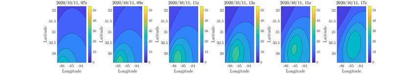
represents the probable trajectories that the hurricane may take.1 In recent history, the realized hurricane track fell

within the cone about 60-70% of the time (Center, n.d.). This suggests that the temporal evolution of the hurricane

track is highly uncertain. Ensemble prediction systems have the potential to significantly improve probabilistic

forecasts of hurricanes by accounting for real-time uncertainties (Majumdar & Finocchio, 2010; Hamill, Whitaker,

Fiorino, & Benjamin, 2011; Lin, Emanuel, & Vigh, 2020) (see Figure 1a).

    The hurricane intensity is typically computed by models such as the Coupled Hurricane Intensity Prediction

System (CHIPS) (Emanuel, DesAutels, Holloway, & Korty, 2004) or FAST intensity simulator (Emanuel, 2017). Then

given a hurricane track and intensity, one can deduce wind velocities at arbitrary locations that may be affected by

the storm, as given by a surface wind field.2 The surface wind field is typically represented by fitting canonical radial

wind distributions to the storm’s forecast intensity and radius of maximum winds (see Figure 1b). Most parametric

wind field models are axisymmetric, i.e., wind velocities are assumed to be equal at equidistant locations from the

storm center (Holland, 1980; Vickery, Skerlj, Steckley, & Twisdale, 2000; Emanuel, 2004; Vickery, Wadhera, Powell, &

Chen, 2009; Chavas, Lin, & Emanuel, 2015). On the other hand, asymmetric wind field models (Xie, Bao, Pietrafesa,

Foley, & Fuentes, 2006; Chang, Amin, & Emanuel, 2020) account for wind variability with respect to both radial

distance and azimuthal angle.3

    Here, we formulate a damage modeling approach that bridges the existing gap in the application of hurricane

models and forecasting methods (Holland, 1980; Vickery et al., 2000; Emanuel, 2004; Emanuel et al., 2004; Xie et

al., 2006; Vickery et al., 2009; Majumdar & Finocchio, 2010; Hamill et al., 2011; Chavas et al., 2015; Emanuel, 2017;

Chang, Amin, & Emanuel, 2020; Lin et al., 2020) to damage estimation. Our probabilistic modeling approach accounts

for the effects of both hurricane forecast uncertainty and spatial variability in wind velocities (see Section 2). To

represent the uncertainty in the forecasted hurricane’s temporal evolution, we employ “Forecasts of Hurricanes using

Large-Ensemble Outputs” (FHLO), which produces 1,000-member forecast track and intensity ensembles (Lin et al.,

2020). To incorporate the effect of spatially-varying wind velocities, we employ a physically-based Nonhomogeneous

Poisson Process (NHPP) model (Brown, Gupta, Christie, Venkata, & Fletcher, 1997; Zhou, Pahwa, & Yang, 2006;

Alvehag & Söder, 2011; Li et al., 2014) for probabilistic damage estimation. The NHPP model outputs spatially-
     1 To form the cone of uncertainty, one estimates the uncertainty in the forecasted track location at each discrete time step. The uncertainty

at a time step is represented by a circle that surrounds the forecasted track location associated with this time. The union of the circles is the cone
of uncertainty, and the cone shape reflects increasing uncertainty with time.
     2 Most wind field models estimate 1- or 10-minute sustained winds.
     3 The difference between the highest and lowest velocities around the radius of maximum winds can readibly be around 10 m/s (Uhlhorn,

Klotz, Vukicevic, Reasor, & Rogers, 2014).

                                                                          4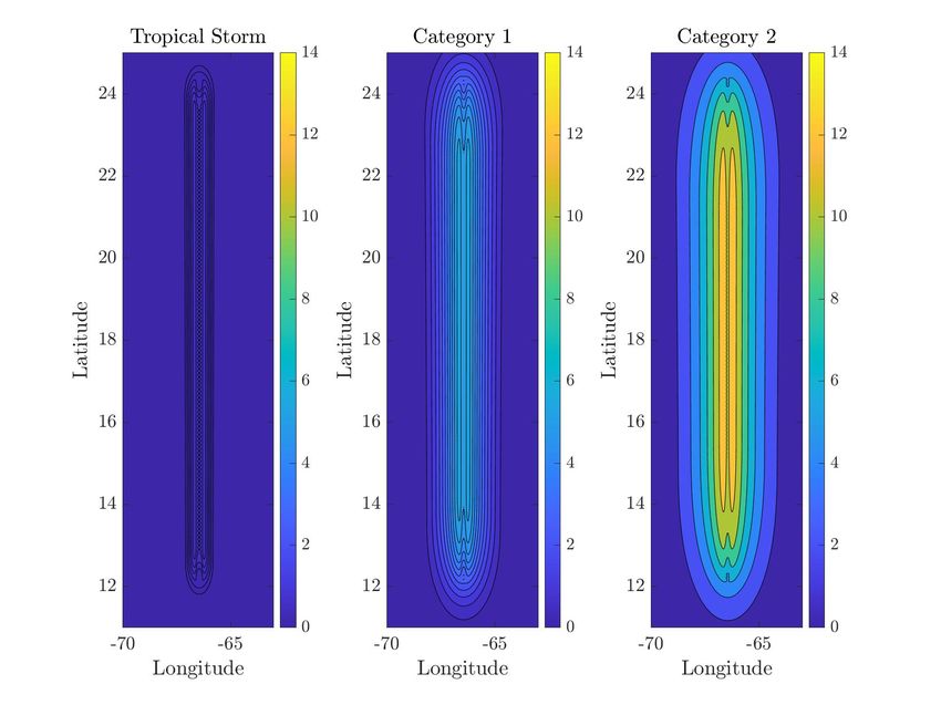
varying probability distributions of the extent of damage (number of asset failures), using a hurricane wind forecast

as input.

    In Section 3, we provide an analysis of the formulated modeling approach. First, we define the “critical zone”

or geographical region that suffers from hurricane wind-induced damage. Then, we assess how spatial variability

in wind velocities and forecast uncertainty represented by FHLO impact the damage estimates. In Section 4, we

apply our modeling approach to the prediction of outages (i.e., loss-of-service) in electric power infrastructure due

to Hurricane Michael. In Section 5, we provide brief insights into how hurricane intensity and size impact total

damage and resulting financial losses. Finally, we provide concluding remarks in Section 6.

2    MODELING APPROACH

In this section, we develop a probabilistic model for estimating spatially-varying damage to overhead assets in in-

frastructure systems. To evaluate damage due to hurricane winds, we estimate a probability distribution over the

number of failed assets in each defined two-dimensional spatial region g P G. In our approach, the location-specific

probability distribution is dependent on the hurricane surface wind field velocities, which are forecasted at each

location g P G and time t P T. The set of times T encompasses discrete time steps between the initial forecast time

t 0 and final forecast time tf , where forecast duration T “ tf ´ t 0 . The times are equally spaced and separated by a

time interval of ∆t.

    We use H “ tvg,t ugPG,tPT to denote the hurricane wind field as a random field, where vg,t defines the velocity

at location g and time t. Furthermore, H g “ tvg,t utPT denotes the velocities corresponding to location g, and

H t “ tvg,t ugPG the velocities corresponding to time t. Henceforth, we will use the notation H̃ to denote a specific

instance of a hurricane wind field, which can be appropriately subscripted using g and t.

    The probabilistic hurricane surface wind field forecast is given by Forecasts of Hurricanes using Large-Ensemble

Outputs (FHLO), which we discuss in Section 2.1. Using a surface wind field forecast (FHLO) as input, we estimate

probability distributions of damage (number of failed assets) within the infrastructure system by employing the

nonhomogeneous Poisson Process (NHPP) model (Section 2.2). Finally, we discuss how the NHPP model can be

integrated with FHLO, in order to account for forecast uncertainties in damage estimates (see Section 2.3).

                                                          5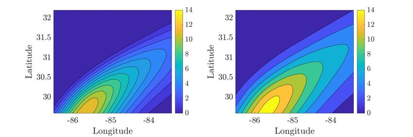
2.1    Forecasts of Hurricanes using Large-Ensemble Outputs (FHLO)

Forecasts of Hurricanes using Large-Ensemble Outputs (FHLO) is a physically-based model framework developed

by Lin, Emanuel, and Vigh (Lin et al., 2020), which generates probabilistic forecasts of the hurricane wind field.

Specifically, FHLO is used to produce probability distributions of wind velocity at fixed locations in space, using a

three-component framework: 1) a track model that bootstraps 1,000 synthetic tracks from the much smaller number

of forecast hurricane tracks from an ensemble numerical weather prediction model; 2) an intensity model that pre-

dicts the maximum wind speed along each synthetic track; and 3) a parametric wind field model that estimates the

time-varying two-dimensional surface wind field along each synthetic track given the position and intensity of the

storm. We use H “ tH̃ piq u@iPt1,...,Hu to refer to a hurricane ensemble obtained from FHLO: the ensemble consists

of H “ 1, 000 ensemble members, where each member is indexed by i and denoted by H̃ piq “ tvg,t ugPG,tPT . The
                                                                                                    piq

empirical probability of the wind field H̃ piq is 1{H.

   FHLO assumes an initialization time at which the forecast begins, typically 1-3 days before the hurricane is

projected to make landfall. Randomness in hurricane tracks and wind velocities stems from forecast uncertainty in

the hurricane track evolution, dynamic and thermodynamic environments, and initial conditions. The probabilistic

intensity forecasts given by FHLO are comparable in accuracy to those of the Hurricane Weather Research and

Forecasting (HWRF) model, an advanced numerical weather prediction model, but also far less computationally

intensive to produce.

2.2    Nonhomogeneous Poisson Process (NHPP) Model

We now focus on generating probabilistic, spatially-varying estimates of damage, using a hurricane wind field H̃ as

input. For each spatial location g P G, we aim to compute a probability distribution over the number of damaged

assets in g accumulated over the set of times t P T. To compute the probability distributions, we employ a Nonho-

mogeneous Poisson Process (NHPP) model, in which the rate of failures is time-varying to reflect the dependence of

infrastructural asset failures on the hurricane wind velocities.

   The NHPP model is used to estimate the Poisson intensities λg,t for locations g P G and at times t P T. The

Poisson intensity is the expected number of failures per unit time, normalized by the asset density. We model the

Poisson intensity λg,t to be a function of the velocity vg,t ; the parametric form of the function depends on the

                                                           6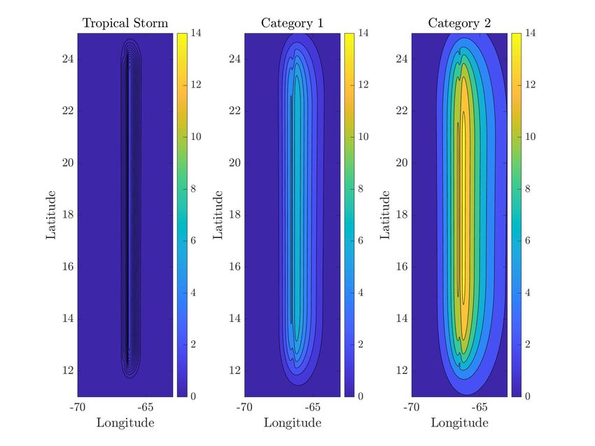
infrastructure system and asset type in question. The Poisson intensities λg,t pvg,t q for t P T can be used to compute

the failure rate Λg , the expected number of failures in g accumulated over the hurricane’s lifetime and normalized

by the asset density:
                                                             ÿ
                                               Λg pH g q “          λg,t pvg,t q ∆t,                                    (1)
                                                             tPT

where ∆t is the time spacing between each time t P T. A typical measure of ∆t is one hour.

     Both the Poisson intensity and failure rate are measures of expected damage when the number of assets per

location can be treated as a large number (infinite). Under this assumption, the probability that there are sg failures

in location g, normalized by asset density, is given by the Poisson distribution:

                                                                    s
                                                                Λgg
                                               Prpsg | Λg q “        expp´Λg q,                                         (2)
                                                                sg !

where Λg , the failure rate, is also referred to as the Poisson parameter.

     If the asset density lg in g is known, then the corresponding “total” failure rate is lg Λg . If we wish to obtain the

distribution over the total number of failures (rather than normalized failures) in a location g, we use lg Λg as the

Poisson parameter in place of Λg . In the example of electricity distribution lines, Λg would be the expected number

of failures per kilometer of distribution lines and lg is the length of distribution lines in kilometers within location

g.

     In reality, the number of assets per location is finite and varies across locations. If there are a finite number of

assets S̄g in a location g, then the distribution over the total number of failed assets must be modified accordingly:
                                            $                                                      ,
                                                      sg
                                            ’  pl Λ  q                                             /
                                            & g s g! expp´lg Λg q,                    for sg ă S̄g /
                                            ’
                                            ’                                                      /
                                                                                                   .
                         Prpsg | lg Λg q “                                                                          (3)
                                                   g

                                            ’                                     x                /
                                                                  S̄   ´1 pl Λ  q
                                                                                    , for sg “ S̄g -
                                            ’                    ř   g      g g
                                                                                                   /
                                               1 ´ expp´lg Λg q x“0
                                            ’
                                            %                                                      /
                                                                             x!

     Hereafter, we refer to the distribution given by Eq. (3) as incorporating “saturation” in the number of failures.

Under this distribution, the expected number of failures Ersg s normalized by asset density is not given by S̄g Λg , but

rather by:
                   S̄g                    S̄g ´1
                                                                                 «                 S̄g ´1
                                                                                                                 ff
                   ÿ                       ÿ         plg Λg qx                                       ÿ plg Λg qx
        Ersg s “         x Prpsg “ xq “            x           expp´lg Λg q ` S̄g 1 ´ expp´lg Λg q
                   x“0                     x“0
                                                         x!                                         x“0
                                                                                                           x!
                                                                                                                        (4)
                                      S̄g ´1                              S̄g ´1
                                    ÿ plg Λg qx´1                           ÿ plg Λg qx
               “ lg Λg expp´lg Λg q               ` S̄g r1 ´ expp´lg Λg q               s,
                                    x“1
                                        px ´ 1q!                           x“0
                                                                                  x!

where Prpsg “ xq is the probability of x events as given by the Poisson distribution in Eq. (3). Figure 2 demonstrates

                                                                7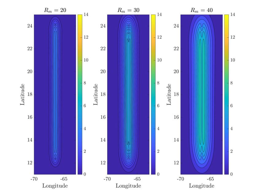
how incorporating saturation affects the expected number of failures Ersg s in a location g, following Eq. (4). Notice

that Ersg s asymptotically approaches S̄, the total number of assets in g. In this case we consider a location with

S̄g “ 30 distribution lines (3 kilometers of lines in the location, where each line has a length of 100 meters).

    In this work, we focus on an NHPP model for hurricane wind-induced failures of overhead infrastructural assets

in electricity distribution systems. In particular, failures of electricity distribution lines are a frequent cause of outages

in power systems (Campbell, 2013), and typically result from downing of supporting poles or toppling by nearby

trees. A standard means of modeling the Poisson intensity for failure of overhead assets is to use a quadratic function

(Brown et al., 1997; Alvehag & Söder, 2011; Li et al., 2014) or exponential function (Lallemand, 2008). In this work,

we focus on a quadratic model for Poisson intensity λg,t , the expected number of failures per hour and kilometer of

assets (i.e., distribution lines):
                                                 $
                                                          vg ,t 2
                                                 ’ ´   ´´       ¯     ¯¯
                                                                        λnorm , if vg,t ě Vcrit
                                                 ’
                                                 & 1`α
                                                 ’
                                                          Vcrit   ´ 1
                                λg,t pvg,t q “                                                                                                  (5)
                                                 ’
                                                                                                if vg,t ă Vcrit .
                                                 ’
                                                 % λnorm ,
                                                 ’

A quadratic function reflects the fact that the pressure exerted on trees and poles is a function of the wind velocity

squared. The model’s key physically-based feature is the quadratic relationship between λg,t and vg,t when vg,t is

greater than the so-called critical velocity Vcrit . For velocities below Vcrit , the infrastructure system only suffers from

a fixed nominal failure rate of λnorm .4 The parameter α is a scaling parameter that controls for the increase in failure

rate with velocities above Vcrit . All three model parameters (Vcrit , λnorm , and α) are dependent on the asset type and

properties (i.e., height, age, material composition). For the remainder of this article, we use the following parameter

values (adapted from (Li et al., 2014)): Vcrit “ 20.6 m/s, α “ 4175.6, and λnorm “ 3.5 ˆ 10´5 failures/hr/km.5

    The equation can be rewritten accordingly, to separate the constant term and velocity-dependent term:

                                           λg,t pvg,t q “ λnorm p1 ´ αq ` λnorm αf 2 pvg,t q,                                                   (6)

    where
                                                                      maxpVcrit , vg,t q
                                                       f pvg,t q “                       .                                                      (7)
                                                                          Vcrit

     4 Literature has suggested that V
                                        crit is 8 m/s, when using historical Swedish weather data in which velocities did not exceed 20 m/s (Alvehag
& Söder, 2011), In contrast, Vcrit was estimated to be 20.6 m/s when using velocities from historical hurricanes up to Category 2 intensity on the
Saffir-Simpson scale (Li et al., 2014).
     5 Other considerations such as precipitation and soil cover have also been shown to be relevant to modeling of failures and outages, but we

focus solely on the variability of Poisson intensities due to the hurricane wind velocities.

                                                                         8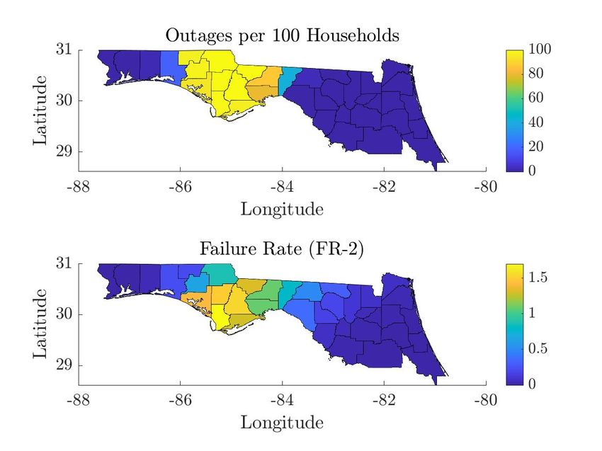
Using Eq. (1), the failure rate Λg for all g P G is given by:

                                                                                                ÿ
                                       Λg pH g q “ λnorm Tp1 ´ αq ` λnorm α∆t                        f 2 pvg,t q.                 (8)
                                                                                               tPT

   Previous applications of the presented quadratic model (Zhou et al., 2006; Alvehag & Söder, 2011; Li et al., 2014)

did not evaluate the spatial variability in estimated Poisson failure rates due to the physical structure of the hurricane

wind field, even though hurricane wind velocities vary significantly with space and time. In contrast, our approach

incorporates spatiotemporal variabilities in winds to estimate the Poisson failure rates. We are also readily able to

replace the quadratic model with an exponential model for the Poisson intensity within the modeling approach.

Furthermore, it is worth noting that our estimated failure rates use wind velocity inputs at one-hour intervals, as

opposed to intervals of 3+ hours in the abovementioned applications of the quadratic model.

   In Section 4, we will discuss how saturation in Eq. (3)-(4) and the critical velocity parameter in Eq. (5) are reflected

in outages resulting from Hurricane Michael.6 We note that a cubic function for the Poisson intensity is suitable if

the effects of blowing debris are considered (Emanuel, 2011). The effect of using different Poisson intensity functions

could also possibly be examined using real-life failure or outage data.

2.3       Integrating FHLO and NHPP Model

We discuss how to incorporate hurricane forecast uncertainty, as given by FHLO, in estimating (i) failure rates and

(ii) failure distributions using the quadratic NHPP model in Section 2.2. In contrast, previous works (Zhou et al., 2006;

Alvehag & Söder, 2011; Li et al., 2014) did not incorporate hurricane forecast uncertainties in failure rate estimation,

in addition to not analyzing how failure rates are affected by wind velocity variability.

   First we define the expected velocity, denoted v̄g,t in location g at time t, under a given hurricane ensemble H

with H ensemble members:
                                                                                       H
                                                                                    1 ÿ piq
                                                         v̄g,t “ Ervg,t s “              v ,                                      (9)
                                                                                    H i“1 g,t
            piq
where vg,t is the velocity in grid g at time t, for ensemble member i. For notational convenience, we use ErH g s to

denote tv̄g,t utPT and ErHs to denote tv̄g,t ugPG,tPT .

   One can consider two ways to incorporate FHLO in estimating failure rates:

   6 It   is also possible to account for saturation directly in the Poisson intensity function, rather than using Eq. (3)-(4).

                                                                            9
• Failure Rate 1 (FR-1): the failure rate as a function of the ensemble-averaged wind velocities, denoted by

      Λg pErH g sq. Using Eq. (1), FR-1 for a location g can be written as:

                                                                ÿ
                                              Λg pErH g sq “          λg,t pv̄g,t q∆t.                           (10)
                                                                tPT

      Then, using Eq. (8), FR-1 under the quadratic NHPP model can be written as:

                                                                                    ÿ
                               Λg pErHg sq “ λnorm Tp1 ´ αq ` λnorm α∆t                   f 2 pv̄g,t q.          (11)
                                                                                    tPT

    • Failure Rate 2 (FR-2): the ensemble-averaged failure rate, denoted by ErΛg pHg qs. Using Eq. (1), FR-2 for a

      location g can be written as:
                                                               H
                                                            1 ÿ
                                           ErΛg pHg qs “         Λ pH̃ piq q
                                                            H i“1 g g
                                                             H
                                                                                                                 (12)
                                                          1 ÿÿ          piq
                                                        “          λ pv q∆t.
                                                          H i“1 tPT g,t g,t

      Then, using Eq. (8), FR-2 under the quadratic NHPP model can be written as:
                                                                                     H
                                                                                  1 ÿ ÿ 2 piq
                              ErΛg pHg qs “ λnorm Tp1 ´ αq ` λnorm α∆t                      f pvg,t q
                                                                                  H i“1 tPT
                                                                                                                 (13)
                                                                                   ÿ
                                                                                             2
                                           “ λnorm Tp1 ´ αq ` λnorm α∆t                  Erf pvg,t qs.
                                                                                  tPT

   FR-1 is computed using the ensemble-averaged velocities, and thus variability in the velocities across ensemble

members is not accounted for. In contrast, FR-2 is obtained using the failure rate for each ensemble member; each

failure rate is computed using the ensemble member-specific velocities as input. Thus FR-2 more properly incorpo-

rates uncertainty in the wind field, as represented by the variability in velocities across ensemble members. In this

work, we compute both FR-1 and FR-2 for historical hurricanes, then compare the differences. The following result

shows that FR-2 is greater than or equal to FR-1:

Proposition 2.1. For a location g and wind velocities Hg , the following holds for the failure rate Λg :

                                              ErΛg pHg qs ě Λg pErHg sq                                          (14)

   The proof of Proposition 2.1 is provided in Appendix A, and requires a simple application of Jensen’s inequality.

   Next we define two estimates of the failure distribution in a location g, which incorporate FHLO. In defining

the distribution estimates, we assume a very large (infinite) number of assets, in order to focus on the relationship

                                                           10
between wind velocities and the failure distributions rather than the effect of infrastructure-specific characteristics
(i.e., number of assets).
Let Prpsg | xq refer to the Poisson distribution given by Eq. (2), which determines the number of failures sg in
location g under Poisson parameter x. Then, the distribution estimates are given as follows:
• Failure Distribution A (FD-A) is given by Prpsg | ErΛg pHg qsq, i.e., the Poisson distribution with the ensemble-
averaged failure rate (FR-2) as the distribution’s Poisson parameter.
• Failure Distribution B (FD-B) is an ensemble-averaged distribution obtained as follows: First, for each en-
semble member i, we obtain a Poisson distribution which uses Λg g q as the Poisson parameter.
piq
“ Λg pH̃ piq
Then, the probability that there are sg failures in grid g is given by:
H
1 ÿ
Prpsg q “ Prpsg | Λpiq
g q (15)
H i“1
i.e., we consider that the distribution given by parameter Λg for ensemble member i occurs with probability
piq
1{H. This is a valid probability distribution because the probability mass owing to each ensemble member is
1{H and there are H ensemble members.
FD-A is computed using the ensemble-averaged failure rate (FR-2), and thus variability in the failure rates across
ensemble members is not accounted for. In contrast, FD-B is obtained using the ensemble member-specific Poisson
distributions, which are parameterized by the ensemble member-specific failure rates. Thus FR-2 more properly
incorporates wind field uncertainty that is represented by the empirical distribution of ensemble failure rates.
3 ANALYSIS
In this section, we analyze how spatial variability in the hurricane wind field and forecast uncertainties given by
FHLO affect the NHPP-estimated failure rates. First we quantify the spatial extent of damage, as measured by what
we define as the “critical zone” (see Section 3.1), the geographical region in which failure rates exceed a defined
threshold. Then we analyze how varying hurricane parameters such as intensity, size, and asymmetries affect the
critical zone area and asset density-normalized failure rates (see Section 3.2). Finally, we assess how forecast un-
certainty affects the probabilistic estimates of infrastructure damage, using wind field forecasts given by FHLO for
11Hurricanes Hermine and Michael (see Section 3.3).
3.1 Hurricane Critical Zone
For this subsection, we consider a simple, stylized axisymmetric model in which the hurricane track deterministically
moves in a straight line from a defined initial (genesis) point xh0 to final (lysis) point xhf . The hurricane travels at a
constant rate given by Vtr , the hurricane translation speed. For a time duration t after hurricane genesis, the track
location is xht “ xh0 ` Vtr t. The parameters xh0 , xhf , and Vtr are length-2 vectors, to separately model the hurricane’s
north-south and east-west movement.
Given the hurricane track, we estimate the wind field H̃ “ tvg,t ugPG,tPT , which consists of velocities defined
at grids g P G and times t P T. Here, T “ tt0 , ..., tf u, where hurricane genesis occurs at time t0 in location xh0 and
dissipates at time tf in location xhf . We assume that the wind field at a time t, defined as H̃ t “ tvg,t ugPG , is given by
the parametric Holland model (Holland, 1980). In the Holland model, the velocity vg,t is a function of radial distance
rg,t from the storm center:
´ R ¯B{2 ´1´ ´ R ¯B ¯¯
m m
vg,t prg,t q “ Vm exp 1´ , (16)
rg,t 2 rg,t
where rg,t “ xg ´ xht 2
(L2 norm) and xg denotes the centre-point of grid g. The Holland model has three
wind field parameters, namely maximum intensity (Vm ), radius of maximum winds (Rm ), and shape parameter (B).
The maximum intensity Vm is the maximum velocity in the surface wind field. The radius of maximum winds Rm
is the radial distance at which the hurricane’s velocity reaches Vm , and is a measure of hurricane size. The velocity
increases with radius rg,t for rg,t ă Rm , and decreases with increasing rg,t for rg,t ą Rm . The shape parameter B
governs the rate of decay of the wind velocities. Here, we assume that the Holland parameters remain constant for
the duration of the storm and B “ 1.7
Next, we define the so-called hurricane “critical zone”, a measure of the spatial extent of hurricane-induced
damage:
Definition 3.1. Consider a hurricane wind field H̃ t at time t for which the maximum intensity Vm ptq ě Vthres , where
7 Typically B is between 1 and 2.5.
12Vthres is a defined threshold velocity. Then the critical zone of H̃ t consists of all spatial locations g P G for which (1)
radius rg,t ă Rm ptq; or (2) rg,t ě Rm ptq and vg,t ě Vthres , where Rm ptq is the radius of maximum winds at time t.
Furthermore, the critical zone of the entire wind field H̃ consists of the union of the critical zones for the time-specific
wind fields H̃ t , @t P T.
If a wind field H̃ t at time t is axisymmetric, then the wind velocity vg,t is only dependent on radial distance rg,t
and we can define a so-called “critical radius”:
Definition 3.2. Assume that for an axisymmetric hurricane wind field H̃ t at time t, Vm ptq ě Vthres . Then, the
critical radius Rcrit pVthres , tq is defined as a radius r ě Rm at which the velocity v “ Vthres .
Note that if the maximum intensity Vm ptq ă Vthres at time t, then the wind field H̃ t does not have a critical
zone or critical radius.
According to Definitions 3.1-3.2, the critical zone of an axisymmetric wind field H̃ t consists of all spatial lo-
cations g for which the radius rg,t is less than the defined critical radius Rcrit pVthres , tq. We now present a simple
result, under the restriction that we consider the simple, stylized axisymmetric hurricane model:
Lemma 3.3. Assume that a hurricane has a straight-line track and constant translation speed Vtr . Furthermore, the
hurricane has a Holland wind field given by Eq. (16) with constant Holland parameters, maximum intensity Vm ě
Vthres , and a defined critical radius Rcrit pVthres q (with a slight abuse of notation, Vm and Rcrit are constant with time
and thus not a function of t). Then, the critical zone of a hurricane wind field H̃ forms an obround with area Acrit given
by:
Acrit “ 2Rcrit pVthres qT kVtr k2 ` πrRcrit pVthres qs2 , (17)
where T is the hurricane lifetime, the obround’s rectangle length T kVtr k2 is the distance covered by the hurricane
track, and the rectangle width is given by two times the critical radius Rcrit pVthres q. The first half-circle at one end of
the obround corresponds to one-half of the critical zone area for the hurricane at genesis. The second half-circle at the
other end corresponds to one-half of the critical zone area for the hurricane at lysis.
For the remainder of the paper, we will focus on the quadratic NHPP model and set Vthres “ Vcrit , where Vcrit
is the model’s critical velocity parameter. This case is particularly important, because the Poisson intensity is equal
to λnorm when the hurricane velocity is below Vcrit . Under this specific model, we present a further result:
13Proposition 3.4. For the quadratic NHPP model given by Eq. (5) and the parameter Vthres “ Vcrit , the failure rate
Λg ą λnorm T if and only if a spatial location g falls in the critical zone of an axisymmetric hurricane H̃ with duration
T.
Proof. If location g is not in the critical zone of H̃, then the Poisson intensity λg,t “ λnorm at all times t P T and thus
Λg “ λnorm T. If g is in the critical zone of H̃, then the velocity vg,t ą Vcrit for at least one time t P T (following
Definitions 3.1-3.2). Since velocity vg,t exceeds Vcrit , we have λg,t ą λnorm and from Eq. (8), we conclude that
Λg ą λnorm T.
The results given by Lemma 3.3 and Proposition 3.4 will be relevant in the next subsection, where we compute
the critical zone area and failure rates under the simple, stylized axisymmetric model we consider here.
3.2 Analyzing Spatial Variability of Damage
In this subsection, we discuss how the critical zone area and spatial variability of estimated failure rates are dependent
on the hurricane parameters of maximum intensity Vm and radius of maximum winds Rm . Then we discuss how
introducing asymmetries (Uhlhorn et al., 2014; Chang, Amin, & Emanuel, 2020), or variabilities in wind velocity with
respect to the azimuthal angle8 , would alter the critical zone and failure rates.
Figure 3 (resp. Figure 4) illustrates the dependency of the critical zone and failure rates on maximum intensity
Vm (resp. radius of maximum winds Rm ), for an axisymmetric wind field. Figure 5 demonstrates how the critical
zone and failure rates vary with Vm , when we introduce an asymmetry by adding the storm-translation vector to
the Holland wind field.9 In this case, the maximum velocity under equal radius occurs at exactly 90˝ clockwise of
the translation direction, where the storm motion and cyclostrophic wind direction are aligned. This is reflected in
Figure 5, where the storm is translating northward, the maximum failure rates occur in a wall east of the storm track,
and the critical zones no longer display the obround shapes suggested by Eq. (17).
Tables 1-3 respectively list the critical zone area Acrit , maximum failure rate, and average failure rate within
the critical zone under varying values of Vm and Rm , for hurricane wind fields with or without asymmetries. Fur-
thermore, in Appendix B, we formulate parametric models that relate the Holland parameters to critical radius and
8 Azimuthal
angle is measured as degrees clockwise from a defined reference direction (typically the storm translation direction)
9 Storm
translation and wind shear are considered important environmental variables in determining the physical structure of a storm’s
asymmetries. Asymmetries can also be accounted for by setting a Holland parameter, such as Vm , to be a function of these environmental inputs
(Chang, Amin, & Emanuel, 2020).
14critical zone area. Both the critical zone area and maximum failure rate achieved increase with Vm and Rm , but the
rate of increase is faster with respect to Vm . The maximum failure rate is also higher under asymmetric hurricanes,
due to the high wind velocities occurring east of the storm track, as shown in Figure 5. In addition, the discrepancy
in maximum failure rate between the axisymmetric and asymmetric hurricanes increases with Vm . This suggests
that not accounting for asymmetries in hurricane wind field forecasts can lead to significant underestimation of fail-
ure rates due to high-intensity hurricanes. In addition, the average failure rate in the critical zone is greater when
asymmetry is included.
Once the conditions of straight-line hurricane track and time-constant Holland wind field parameters are relaxed,
the critical zone area and variability in failure rates would differ from what is suggested in Figures 3-5. For instance,
hurricane maximum intensity Vm is time-varying, and usually lower at the beginning and end of the hurricane’s
lifetime. Furthermore, the Holland wind field considered here only includes one shape parameter, but additional
shape parameters would affect the decay in wind velocities with radial distance; the updated Holland 2010 model
(Holland, Belanger, & Fritz, 2010) includes more shape parameters.
3.3 Analyzing Effect of Forecast Uncertainty on Damage
Now, we assess how forecast uncertainty given by FHLO affects the NHPP-estimated failure rates and failure distri-
butions.10 Our analysis focuses on 1,000-member ensemble simulations for Hurricanes Hermine (2016) and Michael
(2018); parameters used for the simulations given by FHLO are listed in Table 4. Hermine is a Category 1 hurricane,
whereas Michael is a highly intense, Category 5 hurricane that reached peak maximum intensities of around 70 m/s.
Both hurricanes made landfall in northwestern Florida.
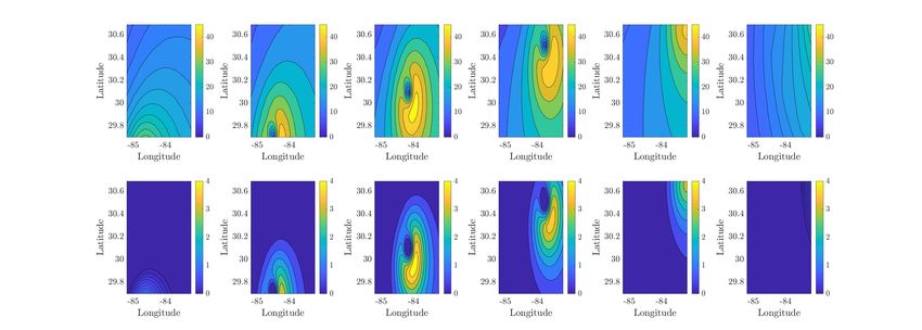
Analysis for Hurricane Hermine: Figure 6 plots Hermine’s wind field H̃ and corresponding Poisson inten-
sities λg,t at six designated times t, for a single ensemble member. Figure 7 plots Hurricane Hermine’s ensemble-
averaged wind field ErHs “ tv̄g,t ugPG,tPT . The velocity contours are much smoother after averaging, and the
majority of the geographical region does not contain significant velocity exceedances above the critical velocity pa-
rameter Vcrit . More specifically, critical velocity exceedances within ErHs occur for only six out of the 121 times
for which the wind field forecast is available.
10 For computation of failure rates (FR-1 and FR-2), we obtain the asset density-normalized failure rate for each grid, then multiple it by the
asset density. We considered The City of Tallahassee Utilities, which has 1,800 km of distribution lines over 255 km2 , averaging to 7.08 km of
line/km2 area (Myers & Yang, July 15, 2020). Furthermore, we assume each location g has an area of 1 km2 .
15Figure 8 demonstrates how spatially-varying failure rates differ depending on the choice of FR-1 vs. FR-2. Recall
that in Section 2.3, we proved FR-2 is greater than or equal to FR-1. When using FR-1 as the failure rate estimate,
only 20.9% of the considered geographical region (4,414 km2 ) falls within the critical zone. In contrast, 100% of the
considered geographical region falls within the critical zone when using FR-2. Furthermore, the region-averaged
failure rate is 0.12 failures/kilometer of assets for FR-1 and 3.34 for FR-2. This suggests that failure rates are, on
average, more than 28 times higher under FR-2. The main reason for this discrepancy is that supercritical velocities
(wind velocities greater than the defined critical threshold Vcrit ) are averaged out if FR-1 is used, whereas FR-2
considers the individual ensemble member wind fields in failure rate estimation. In this sense, FR-2 is more realistic,
as the supercritical velocities in the ensemble member wind fields are accounted for in failure rate estimation.
Figure 9 demonstrates how the probability distribution over the number of failures depends on the choice of
FD-A vs. FD-B. The spatial locations associated with the distributions in Figure 9 differ in terms of minimum radial
distance to the storm center achieved during the hurricane’s lifetime. Both distributions are right-skewed, but FD-B
is especially so: the probability given by FD-B is maximum at zero failures and decreases with increasing number
of failures. Furthermore, FD-B has a more pronounced tail than FD-A. Amongst the four locations, it is anywhere
between 4.6 and 80 times more likely to have nine or more failures when using FD-B in place of FD-A. The difference
in the probability of 9+ failures, as given by FD-A vs. FD-B, is greater for locations that are farther from the storm
track. This suggests that FD-A particularly underestimates the probabilities of high-damage outcomes for locations
in the storm periphery.
Analysis for Hurricane Michael: Figure 10-12 demonstrate how the failure rates given by FR-1 and FR-2
differ for Michael. Due to Michael’s high intensity, its ensemble-averaged wind field contains more frequent and
significant exceedances of the critical velocity (occurring at 26 out of the 121 times) in comparison to Hermine (see
Figure 11). As a result, estimates of FR-1 are also much higher (see Figure 12). The region-averaged failure rate is
2.69 failures/kilometer of assets for FR-1 and 4.48 for FR-2, which implies that the average failure rate is 1.67 times
higher under FR-2. The difference between FR-1 and FR-2 is less pronounced than for Hermine, because Michael is
a high-intensity hurricane and hence a more significant portion of the geographical region falls in the critical zone
under FR-1.
Figure 13 demonstrates how the failure distributions given by FD-A and FD-B differ for Michael. As a result of
16Michael’s high intensity, the probability distributions have more pronounced tails and less right-skewedness than
under Hermine.
4 PREDICTING OUTAGES IN HISTORICAL HURRICANES
A lack of accurate damage predictions can impede estimates of loss-of-service within infrastructure systems. Im-
proved estimation of loss-of-service is desirable in estimating hurricane-induced risk on the infrastructure system,
as well as in informing proactive strategies to maintain post-disaster infrastructural functionality. In Section 3, we
focused on the spatial variability in NHPP estimates of probabilistic damage and effects of forecast uncertainty given
by FHLO. In this section, we consider the relationship between damage and loss-of-service. Specifically, we analyze
the accuracy of estimated NHPP failure rates in predicting loss-of-service within electric power infrastructure result-
ing from Hurricane Michael. For electricity networks, we consider that loss-of-service is given by outages, or loss
of electrical power network supply to customers. The failure rates (FR-2) are estimated using wind field forecasts
given by FHLO as input (see Section 2.3).
We discuss the computational setup in Section 4.1: the application of FHLO and NHPP, the selected geographical
region of interest, and the outage data employed. Our analysis focuses on the northwestern Florida region (including
the Tallahassee urban area), where Hurricane Michael made landfall. In Section 4.2, we formulate regression models
to predict outages, and demonstrate that a statistically significant relationship exists between the estimated failure
rates and outage rates. In Section 4.3, we discuss insights obtained from studying the estimated regression models.
4.1 Computational Setup
The probabilistic wind field forecast for Michael is given by a 1,000-member ensemble forecast using FHLO. For each
ensemble member, the velocity is forecasted at locations within the latitude range 29.3˝ N to 32.2˝ N and longitude
range 82.6˝ W to 88.7˝ W, with 0.1˝ ˆ 0.1˝ grid spacing. The forecast is initialized on October 9, 2018 at 12Z (Coordi-
nated Universal Time). This time corresponds with around 8:00am Eastern Daylight Time (EDT), which is about 1.5
days before Michael made landfall near Mexico Beach, Florida.
We obtain outage data from the Florida Division of Emergency Management (Ray & Yang, July 23, 2020). Our
analysis focuses on October 10-12, the days during and immediately after Michael’s landfall in Florida. On these
17three days, outage data is available at six different times given in Eastern Daylight Time (EDT): October 10, 15:40;
October 10, 16:35; October 10, 19:50; October 11, 19:40; October 11, 22:00; and October 12, 23:05. At each time, the
outages are measured by number of households without power in each county. The total number of households and
geographical area associated with each county are also included in the data. Using this data, one can compute the
total number of outages per county, the percentage of households experiencing outages, as well as percentage or
number of households with outages normalized by area. We focus on outages in the counties of Northern Florida
(particularly the Tallahassee area).
To compare outages to failure rates (FR-2), we first estimate the failure rates in each county on an hourly basis
using the quadratic NHPP model (Section 2.2). This requires computing the Poisson intensity λg,t using Eq. (5) in
piq
each 0.1˝ ˆ 0.1˝ grid g, at each hour t, and for each ensemble member i. For a grid g, the ensemble-averaged failure
rate Λg pt 1 q at a given time t 1 ď t f (where tf corresponds to Oct. 14 at 12Z, the last time for which FHLO is available)
is given by:
1
H t
1 ÿ ÿ piq
1
Λg pt q “ λ . (18)
H i“1 t“t g,t
0
This summation is similar to Eq. (1), except that the summation is taken over t P tt 0 , ..., t 1 u rather than t P T where
T “ tt 0 , ..., tf u. These failure rates are expected to be increasing with time t 1 , reflecting accumulated exposure of the
electric power infrastructure to hurricane winds over time. Then, we map the grid-wise failure rates to county-wise
failure rates. To do so, we assign a grid to a county, if the majority of the grid’s spatial area is occupied by said
county. We obtain the county-wise failure rate by averaging the grid-wise failure rates corresponding to the county.
We also define the ensemble-averaged “cumulative velocity” at a time t 1 and for grid g as follows:
1
H t
1 ÿ ÿ piq
1
Vg pt q “ v , (19)
H i“1 t“t g,t
0
i.e., it is the ensemble-averaged sum of the grid-specific velocities over all measurement times from t 0 to t 1 . Next
we compute county-wise cumulative velocities, using the same procedure that we applied to the failure rates. The
county-wise failure rates and cumulative velocities are used as inputs to regression models that predict outage rates.
In Figure 14, we plot the outage rates (number of outages per 100 households) and asset density-normalized
failure rates (FR-2) in Northern Florida at four different times. Failure rates are calculated using Eq. (18). Figure 14a
plots the outages and failure rates about three hours after Hurricane Michael made landfall in Florida. In contrast,
18Figure 14d shows the results nearly 33 hours after landfall. The counties with high outages rates mostly fall in the
critical zone of the hurricane, which corresponds to the counties where the failure rates are higher (denoted by light
blue, green, orange or yellow colors), as opposed to sub-critical regions corresponding to dark blue. In particular,
the highest outage and failure rates mostly occur in the geographical region between Panama City and Tallahassee.
4.2 Outage Rate Prediction via Regression Models
We estimate regression models that relate outage rate (outages per 100 households) to one of two inputs: failure rate
(FR-2, Eq. (18)) or cumulative velocity (Eq. (19)). The cumulative velocity is employed in order to analyze the extent to
which the critical velocity Vcrit affects the outage prediction. According to the quadratic model, Poisson intensities
are small and constant for velocities below Vcrit . Thus we hypothesize that failure rates remain insignificant below
a certain cumulative velocity threshold, which translates to near-zero outage rates. Our goal is to evaluate this
hypothesis using the empirical observations of outages.
To assess the strength of cumulative velocities and failure rates as predictors of outage rates, we estimate binomial
regression models (BRMs). In particular, the BRM gives the probability over number of successes out of a set of
Bernoulli trials. In our case, a “success” is an outage and the number of “trials” is given by the number of households
in a given county. We estimate a BRM for each input (cumulative velocity or failure rate) and at each time for which
outage data is available. Figure 15 (resp. 16) plots the outage rate vs. cumulative velocity (resp. failure rate) at four
different times; estimated binomial regression models are included in the plots. We find that cumulative velocity is
a statistically significant predictor (p-value less than 0.05) at all considered times except October 12, 23:05 (about 58
hours after landfall), and failure rate is a statistically significant predictor at all times. For more details regarding
implementation of the BRM, please see Appendix C.
4.3 Discussion
We observe from Figure 15 that the relationship between outage rate and cumulative velocity could be approximately
represented by an S-shaped curve. The outage rate is near-zero and roughly constant for cumulative velocities
below a certain threshold, which is consistent with inclusion of the critical velocity parameter in the NHPP model.
Once this threshold is passed, we observe a rapid increase in the outage rate with cumulative velocity, because of
19the quadratic relationship between Poisson intensity and velocity above Vcrit . Then once the cumulative velocity
becomes sufficiently high, the outage rate approaches 100%, i.e., saturation has occurred (see Eq. (3) in Section 2.2). In
summary, the binomial regression model is able to account for the impact of the critical velocity as well as saturation
on the outage rates.
Figures 14c-14d, which correspond to October 11, illustrate the effect of saturation. Specifically, a few counties
(mostly between Panama City and Tallahassee) have outage rates of around 100% but noticeably differing failure
rates. The variability in failure rates within this region may also result due to the network topology of distribution
feeders in the power infrastructure, which is subject to physical laws and managed by system operators. For ex-
ample, if a substation within a distribution feeder is disrupted, then power supply to all downstream loads will be
interrupted. As another example, failure of a critical asset in the power infrastructure can cause multiple outages,
whereas failure of non-critical assets may not cause any outage if the network is able to survive in the presence of
these failures.
The cumulative velocity-outage rate relationship is not statistically significant on October 12, 23:05, because it
has been over two days since Hurricane Michael made landfall in Northern Florida. Over the course of this time,
Michael traveled northward; there was ample time for utilities to repair damage and restore electricity service. This
suggests that cumulative velocity alone would not be a sufficient predictor of outages at this time, because spatially-
varying repair rates become increasingly important with time.
5 ESTIMATING TOTAL DAMAGE AND FINANCIAL LOSSES
Finally, we estimate parametric models that relate total hurricane-induced damage and financial losses in an infras-
tructure system to two key storm parameters: intensity parameter Vm and size parameter Rm (see Section 3.1). The
parametric models are estimated using the quadratic nonhomogeneous Poisson process (NHPP) model detailed in
Section 2.2, to demonstrate simple power law relationships between damage, financial losses, and hurricane param-
eters (see Figure 17). Here, we assume that hurricanes have the same characteristics as were defined in Section 3.1.11
Parametric Function for Total Damage: While we can formulate an analytical solution for total damage Λtotal
11 We do not employ FHLO in this section; incorporation of FHLO would require us to obtain wind field ensembles from a large number
of historical hurricanes. The computational expense of calculating failure rates from all the ensembles would be high. Furthermore, hurricane
intensity and size will vary temporally in FHLO, which would make estimating the parametric functions less straightforward. However it is also
possible to repeat the exercise conducted in this section using FHLO.
20(see Appendix D.1), it is not convenient to relate the analytical solution to Vm and Rm , due to the highly nonlinear
nature of the Holland model. Consequently, we formulate a parametric function for Λtotal which accounts for the
critical velocity parameter Vcrit and the critical zone area Acrit (see Appendix D.2). With regards to Vcrit , we consider
the following function of Vm as an input to the parametric models:
maxpVcrit , Vm q ´ Vcrit
gpVm q “ (20)
Vcrit
The function gpVm q “ 0 if Vm ď Vcrit , and increases linearly with Vm otherwise.
Based on the estimated model parameters, Λtotal is roughly proportional to R2m and rgpVm qs2.26 when Vm ě
Vcrit , as opposed to the quadratic relationship between location-specific failure rate and velocity in Eq. (5). This
power law relationship can be expressed as:
(21)
` ˘
Λtotal pVm , Rm q „ O R2m pVm ´ Vcrit q2.3 .
Parametric Function for Total Financial Loss: For the purpose of financial loss modeling, we formulate a
network repair model that ensures the financial loss associated with a given location scales quadratically with the
number of local failures (see Appendix E.1). As is the case for total damage, the analytical solution for total financial
loss (see Appendix E.2) cannot conveniently incorporate Vm and Rm as inputs. Instead, we formulate a parametric
model for total financial loss Ltotal that considers the power law relationship for damage suggested by Eq. (21) and
the network repair model in Appendix E.1. Based on the estimated model parameters, Ltotal is roughly proportional
to R3m and rgpVm qs5.6 when Vm ě Vcrit . Because of the quadratic relationship between location-specific financial
loss and number of damages, the polynomial orders associated with Rm and gpVm q for Ltotal are expectedly greater
than those for expected damage Λtotal . The associated power law relationship can be expressed as (see Appendix E.3):
(22)
` ˘
Ltotal pVm , Rm q „ O R3m pVm ´ Vcrit q5.6 .
For Eq. (21)-(22), we do not account for finiteness in the total number of assets. However, in Appendix D.3, we
discuss how computed total damage would differ when saturation is incorporated in the damage estimation.
Previous work (Nordhaus, 2006) has suggested that total hurricane-induced financial losses are roughly a function
of Vm to the 8-th power. In contrast, we estimate the relationship between total financial losses and gpVm q, rather
than Vm . This accounts for our expectation of insignificant damage below the critical velocity Vcrit , which we
21showed is in agreement with empirical observations in Section 4. By using gpVm q as a predictor, we estimate that
total losses are roughly proportional to Vm ´ Vcrit to the 5.6-th power, when Vm ě Vcrit . In contrast, when we
used Vm as a predictor, we found that losses were proportional to Vm to the 7.8-th power.
6 CONCLUDING REMARKS
In this paper, we introduce a modeling approach for probabilistic estimation of hurricane wind-induced damage to
infrastructural assets. Our approach uses a Nonhomogeneous Poisson Process (NHPP) model to estimate spatially-
varying probability distributions of damage as a function of the hurricane wind velocities. The NHPP model is applied
to failures of overhead assets in electricity distribution systems, and features a quadratic relationship between the
Poisson intensity and wind velocity above a critical velocity threshold. In order to incorporate hurricane forecast
uncertainty in estimation of the distributions, we employ Forecasts of Hurricanes using Large-Ensemble Outputs
(FHLO) as inputs into the NHPP model.
The NHPP model’s critical velocity parameter motivates us to define the “critical zone”, a measure of the spatial
extent of hurricane-induced damage. Using a simple model of the hurricane that incorporates the axisymmetric Hol-
land wind field, we demonstrate how the critical zone and failure rates are dependent on hurricane intensity, size, and
asymmetries. Then we show that not incorporating forecast uncertainty given by FHLO results in underestimation
of failure rates, and assess the degree of underestimation under two hurricanes of different intensities (Hermine and
Michael). In addition, we empirically demonstrate that improperly estimating probability distributions of damage
results in underestimation of high-damage scenarios. These findings suggest that forecast uncertainty plays a critical
role in estimation of hurricane-induced damage.
Our modeling approach is able to accurately predict outages resulting from Hurricane Michael. By fitting bino-
mial regression models (BRMs), we demonstrate that failure rate and cumulative velocity are statistically significant
predictors of the outage rate. The fitted BRMs also demonstrate that empirical observations are reflective of the
critical velocity parameter in the NHPP model, and that the outage rates saturate at 100% once failure rates are suf-
ficiently high. Finally, we fit simple parametric models that relate total damage and financial losses to key hurricane
parameters (intensity and size). Under a simple, stylized hurricane model, we show that total damage is proportional
to intensity (resp. size) to the 2.3-th (resp. 2-th) power, and that total financial losses is proportional to intensity
22(resp. size) to the 5.6-th (resp. 3-rd) power.
Future work on this topic will focus on the joint effects of damage and network topology on infrastructure
system loss-of-service. Network topology determines connectivity between the service producers and end-users, as
well as the criticality of various infrastructure assets, such that damage of more critical assets results in an especially
significant loss-of-service. It is also worth noting that this work focuses on hurricane winds, rather than other
relevant physically-based threats induced by hurricanes. These threats, such as storm surge and rainfall, can also
cause substantial damage to infrastructure systems.
A second avenue of future work is to apply improved damage and loss-of-service estimates to the design of
proactive (pre-storm) strategies that minimize hurricane wind-induced risk on infrastructure systems. Accurate es-
timation of spatially-varying damage minimizes risk by not only improving the optimality of proactive strategies,
but also by increasing the efficiency of damage localization and repair. For instance, a plethora of works address
optimal proactive allocation of distributed energy resources (DERs) (Gao, Chen, Mei, Huang, & Xu, 2017; Sedzro,
Lamadrid, & Zuluaga, 2018; Chang, Shelar, & Amin, 2018, 2020) in distribution feeders of electric power infrastruc-
ture; our work is readily applicable to the proposed methods in these works. Indeed, research demonstrates that
energy customers are willing to pay for back-up electricity services during large outages of long duration (Baik,
Davis, Park, Sirinterlikci, & Morgan, 2020).
23You can also read