Supplement of Calibration and assessment of electrochemical low-cost sensors in remote alpine harsh environments
←
→
Page content transcription
If your browser does not render page correctly, please read the page content below
Supplement of Atmos. Meas. Tech., 14, 6005–6021, 2021
https://doi.org/10.5194/amt-14-6005-2021-supplement
© Author(s) 2021. CC BY 4.0 License.

Supplement of
Calibration and assessment of electrochemical low-cost sensors in remote
alpine harsh environments
Federico Dallo et al.

Correspondence to: Federico Dallo (federico.dallo@unive.it)

The copyright of individual parts of the supplement might differ from the article licence.
S1     Techical Specifications

   Purpose of the study is to assess the reliability of low cost sensors for the environmental monitoring of tropospheric Ozone.
   The low-cost monitoring station is located in a remote alpine area, where comparison of data harvested by low cost sensors can
   be compared with state-of-art instrumentations. The sensors evaluated are the Alphasense OX-B431, calibrated prior to field
 5 installation at CNR-ISAC headquarted in Bologna.
      The gas sensor provides three electrodes: the working electrode (WE) where the ozone and nitrogen dioxide react and a
   current proportional to the ozone and nitrogen dioxide concentration is formed; the counter electrode (AUX), twin of the
   working electrode screened from the atmosphere, it reacts to temperature providing a way to correct from temperature depen-
   dance; the reference electrode that anchors the working electrode potential to ensure that it is maintained at a fixed potential,
10 independently from the current generated.
      Each sensor was purchased with its individual sensor board that provides a dual channel voltage output, one for the work-
   ing electrode and one for the auxiliary electrode. These output pins can be interfaced with a commercial Analog to Digital
   Converter.
      The Col Margherita Observatory is a prefabricated insulated shelter with external dimensions of 3.00m x 2.42m x 3.22m.
15 The observatory is equipped with a complete automatic weather station mounted on a 3 m mast (AWS: CS215-L probe, Camp-
   bell Scientific, Utah, USA; PTB110 Barometer, Vaisala, Helsinki, Finland; 05103-45 Wind Monitor, R. M. Young Company,
   Michigan, USA) and an UV-absorption ozone analyser (Thermo Fisher Scientific 49C, SN: 0503110399). The MRG observa-
   tory is unmanned and fully automated, it is connected to the main electrical grid and supplied with a backup solar power system
   with ≈200 Ah batteries in case of grid failure. The observatory is equipped with remote control via GSM / GPRS technology.
20    The sensing system was connected to the main power grid (AC) and to the LTE router of the MRG Observatory to allow data
   communication and remote control. The sensing system was equipped with an uninterruptible power supply (lead acid battery
   and battery charge regulator) in case of AC failure. The processing unit of the sensing system was a Raspberry Pi 3b+ and the
   analog signal of the sensors were digitized using a ± 5V (16 bit) ADC converter (Texas Instruments ADS1115).

     S1.1    Components

25   The dimension of the IP56 box is 300x220x120 mm, the total dimension of the wooden cover is 360x290x180 mm. Three
     arrows on the bottom of the box indicate where the Ozone sensors are located. To open the box it is necessary a ≈10 mm
     flat-blade screwdriver. Inner object are:
          1. AC power wires (red and black are phase and neutral, yellow/green is the Ground),
          2. ethernet wire to bring internet connection to the Raspberry Pi (7b),
30        3. power supply, AC input and 12 VDC out, where black is V- ad red V+,
          4. charge regulator, 12 VDC input from power supply into the “Solar” socket, VDC input/output from the 12 V “Battery”
             and 12 VDC output from “Load” to the DC/DC (6). Black is V- ad red V+.
          5. 12 V, 2,3 Ah battery that acts as an UPS in case of AC failure. It is connected to the “Battery” on the charge regulator
             using black as V- and red as V+.
35        6. DC/DC. 12 VDC input from che charge regulator and 5 VDC output to the Raspberry Pi,
          7. a) USB power wire for the b) Raspberry Pi,
          8. Data acquisition board. This board contains the circuit that performs analog to digital conversion of the sensor’s mea-
             surements and then send digital data to the Raspberry Pi using i2c protocol.
          9. Ozone sensor made by Alphasense,
40    10. sensor plug for ease the change of the sensor,
      11. this is a spare sensor which is not measuring. It is calibrated like the others.

                                                                      1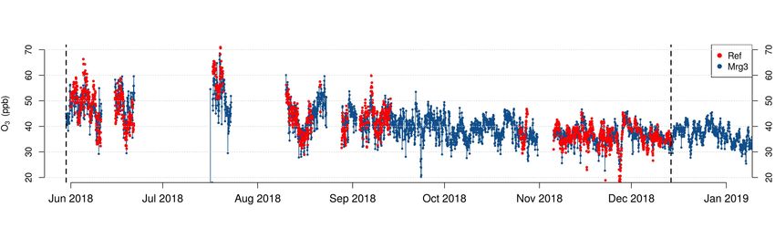
Figure S1.1. The Raspberry Pi with the GPIO on the left. The schematic of the pins are shown in Figure S1.4.

     S1.2   Wiring Raspberry Pi with the acquisition board

     The most tricky operation in case of maintenance could be the correct wiring of the acquisition board and the T&RH sensors
     to the Raspberry Pi. In Figure S1.1, Figure S1.2 and Figure S1.3 are shown the wires that goes to the Raspberry Pi, while
45   Figure S1.4 shows the pins scheme of the Raspberry Pi. Here is the list of connection from acquisition board to Raspberry Pi:
         – RED on 5 V, pin04
         – BROWN on GND, pin06

         – GREEN on SDA, pin03
         – BLUE on SCL, pin05
50   Here is the list of connection from T&RH on the top of sensor 1 (it has a 1 on it) to Raspberry Pi:

         – RED on 3.3 V, pin01
         – WHITE on GND, pin09
         – YELLOW on GPIO22, pin15
     Here is the list of connection from T&RH on the top of the acquisition board (it has a 4 on it) to Raspberry Pi:

55       – RED on 3.3 V, pin17
         – WHITE on GND, pin30
         – YELLOW on GPIO23, pin16

                                                                        2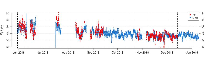
Figure S1.2. A detail of the wiring between the acquisition board and T&RH sensors to the GPIO of the Raspberry Pi. Here are shown the
     GPIO pins from 1 (bottom-right) to 24 (top-left).

     S1.3   Mounting the sensors

     Each sensor is fastened with eight Phillips screws, four from the inside and four from the outside. In Figure S1.5 you can see
60   that each sensor is provided of four spacers and stainless steel flat washers. From the outside there are four rubber gaskets to
     protect from humidity that may come into the box.
        The main hole that get the sensor in contact with air is also provided with a gasket ring.
        Mounting and unmounting the sensor is easy, just remove the sensor plug and then unscrew from outside the box.

     S1.4   Wiring sensors with the acquisition board

65   As shown in Figure S1.5, sensors are wired using a numbered plug. In case of need to change the sensor the procedure should
     be straightforward; unplug the sensor, unscrew it using the Phillips screwdriver and the wrench, replace it with the new sensor
     and plug it.

                                                                       3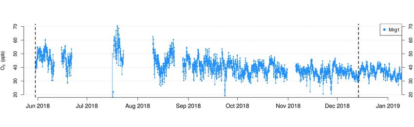
Figure S1.3. A detail of the wiring between the acquisition board and T&RH sensors to the GPIO of the Raspberry Pi. Here are shown the
     GPIO pins from 9 (GND with white wire on bootom-right of the pic) to 30 (GND with white wire on top-left of the pic).

     S1.5   Replacing the power supply

     First remove the power connector from the outer left side of the box, in order to avoid 220 VAC. Then it is possible to detach
70   the power supply from its support, removing the two flat-blade screws that are beneath it. After removing the power supply,
     it should be easy to remove all the wires (phase input, neutral input, ground, V+ output and V- output) with the Phillips
     screwdriver. At this point, replace the power supply with the spare part and rewire. Prior to wire the power supply to the charge
     regulator, be sure that the V+ output don’t exceed 13.5 V and is not less than 12.5 V. Voltage output can be adjusted with the
     Phillips screwdriver.

75   S1.6   Replacing the charge regulator

     Remove all the red(V+) and black(V-) wires from the terminal blocks “mammuth”, only the regulator side has to be released.
     Then remove the two Phillips screws and replace the charge regulator with its spare part.

                                                                       4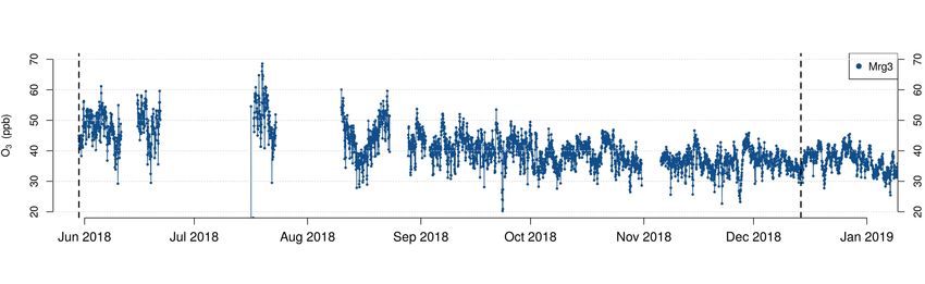
Figure S1.4. This is the scheme of the Raspberry Pi GPIO pins. Check if you’re looking with the right orientation (in Figure S1.1 the pin
1 is on the bottom-right). This "table showing all 26 pins on the P1 header, including any special function they may have," was made by
SparkFun and can be reused under the CC BY licence.

Figure S1.5. These are the three working sensors, and the T and RH sensor close to Sensor 1.

                                                                    5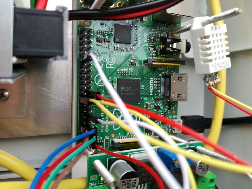
S1.7    Replacing the battery

      Remove the red(V+) and black(V-) wires from the terminal blocks “mammuth” from the battery side. Cut the cable ties and
80    then the battery can be changed with a new one.

      S1.8    Replacing the DC/DC

   The DC/DC is fixed with dices. It is sufficient to remove the dice and then pull out the board. Release the wires using the
   Phillips screwdriver and then replace the DC/DC with the new one.
      WARNING: before to give power to the Raspberry Pi, check that the VDC output is 5.0 VDC (4.75V < Vout < 5.25V is
85 fine)!!! You can regulate output voltage with the screw on the blue resistor.

      S1.9    Replacing the Raspberry Pi USB power wire

      Release the wire from the DC/DC output then remove the µUSB from the Raspberry Pi and replace with the new cable.

      S1.10    Replacing the acquisition board

      Hoping that you’d never arrive to this... To remove the acquisition board first remove each sensors plug. Then remove all the
90    wires from the Raspberry Pi pins. Once free, remove the T&RH sensor and then the dices that keep the acquisition board in
      place. Then replace the board with the new one and follow the subsection S1.2 to rewire everything.

      S1.11    Replacing the Raspberry Pi

   To remove the Raspberry Pi you have to remove its power USB wire and the ethernet wire, then remove the T&RH sensor and
   the acquisition board. Therefore you can remove the dices that lock the Raspberry Pi. The new Raspberry Pi has everything
95 preinstalled so that, once repowered and connected to the Internet, it should automatically be part of the VPN that allows for
   remote control.

      S1.12    Approximate cost of the sensing system

      The sensing system cost is around 700 EU. Considering the following prices:
         – O3 Alphasense sensors 3*150 EU;
100      – Lead acid battery 20 EU;

         – charge regulator 20 EU;
         – DHT22 sensor 2*20 EU;
         – DC/DC step down 10 EU;
         – ADS1115 ADC 16 bit 2*15 EU;

105      – Raspberry Pi 40 EU
         – IP56 box 40 EU
         – Breadboard and wires about 50 EU

                                                                   6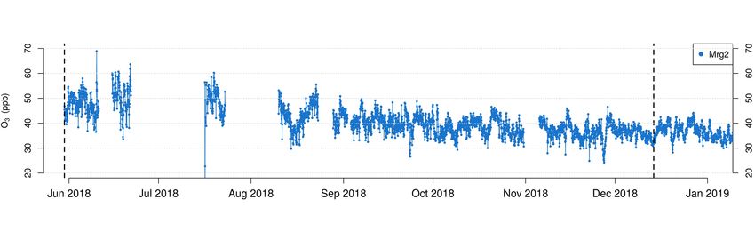
S2   Filtering LCS dataset

Figure S2.1. Example of the automaitic filter to detect outliers in the dataset collected during laboratory calibration.

Figure S2.2. Example of the automaitic filter to detect outliers in the field dataset.

Figure S2.3. The behaviour of the Mrg2 sensor was not consistent in respect to the others LCSs from 1AM November 5 to 11PM November
8. We were not able to identify the cause of this temporary malfunction, but it represents an interesting event proving the importance of
considering low-cost sensors redundancy. The data from Mrg2 flagged as erroneous readings were excluded from the dataset and statistical
analysis

                                                                        7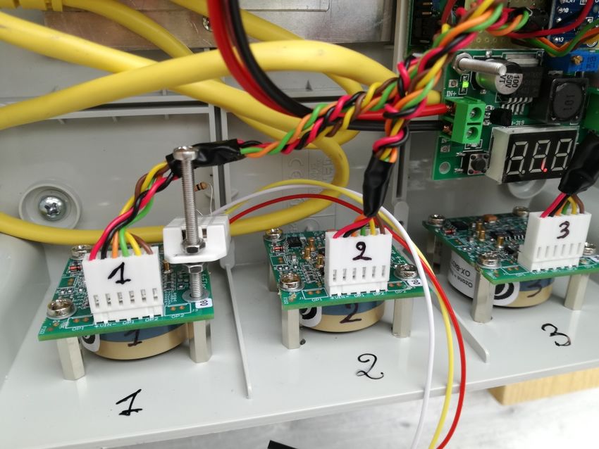
S3   Electrical noise

Figure S3.1. Electrical noise of the LCSs.

                                             8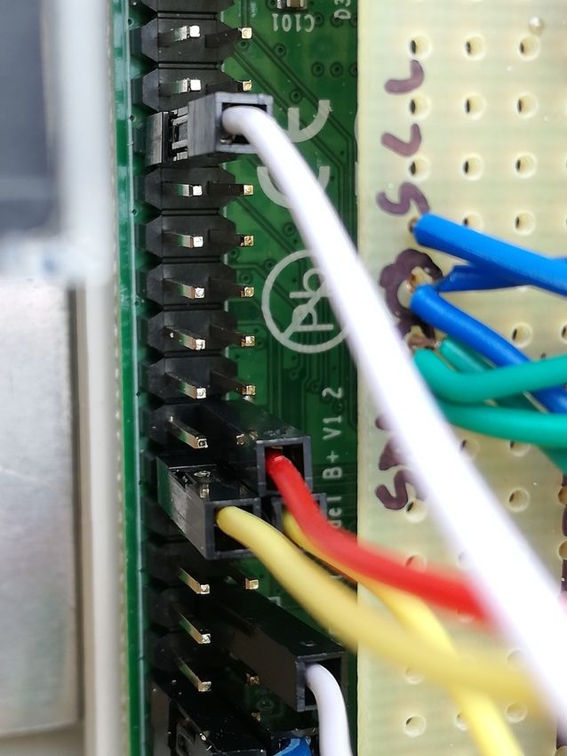
110   S4   Laboratory calibration of LCSs

      The mean voltage response of Mrg2 was 0.8 ± 0.7 mV, when reference ozone concentration was 0.4 ± 0.1 ppb, and reached
      89.3 ± 0.9 mV when reference ozone concentration was 250.2 ± 0.3 ppb. Precision of the Mrg2 sensor was 3.5% for values
      close to the LOD and decreased to 0.9% for ozone concentrations higher than 200 ppb. Mrg2’s MAE was 2.5 ppb, LOD was 5
      ppb, LOQ was 17 ppb and LDR was 5-250 ppb (R2 = 0.999). The mean voltage response of Mrg3 was 38.3 ± 0.9 mV, when
115   reference ozone concentration was 0.4 ± 0.1 ppb, and reached 123.5 ± 0.9 mV when reference ozone concentration was 249.7
      ± 0.2 ppb. Precision of the Mrg3 sensor was 2.6% for values close to the LOD and decreased to 0.7% for ozone concentration
      higher than 200 ppb. MAE for Mrg3 was 2.6 ppb. Mrg3’s LOD was 3 ppb, LOQ was 9 ppb and LDR was 3-250 ppb (R2 =
      0.998).

      Figure S4.1. The RSD for the LCSs is lower for higher ozone concentration.

                                                                        9
S5 Ozone measurements and meteorological variables in Col Margherita
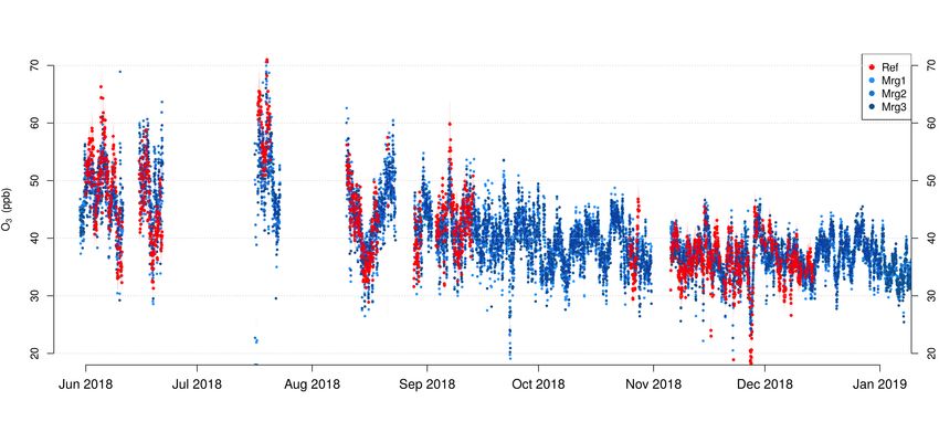
Figure S5.1. Time series of ozone concentration measurements and meteorological variables for the period June-December 2018. The first
plot from the top show the LCSs ozone concentration (ppb) in blue and the reference ozone concentration (ppb) in red. The second plot
shows the external air Temperature (T). The third plot shows the Retive Humidity (RH). The third plot shows the Atmospheric Pressure (P)
and the fourth plot shows the Wind Speed (WS). It is clearly visible the Vaia storm event that hit the North-eastern Italy on 29th October.
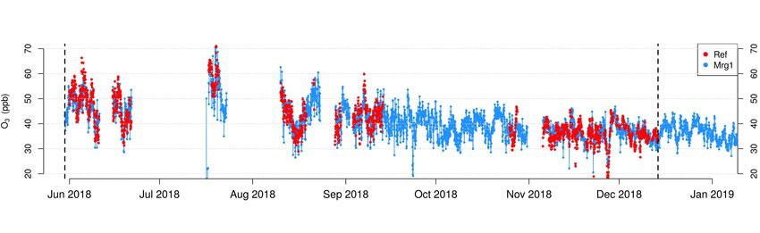
10Figure S5.2. Time series of ozone concentration measurements and meteorological variables for the period June-December 2018. The first
plot from the top show the Mrg1 ozone concentration (ppb) in blue and the reference ozone concentration (ppb) in red.
11Figure S5.3. Time series of ozone concentration measurements and meteorological variables for the period June-December 2018. The first
plot from the top show the Mrg2 ozone concentration (ppb) in blue and the reference ozone concentration (ppb) in red.
12Figure S5.4. Time series of ozone concentration measurements and meteorological variables for the period June-December 2018. The first
plot from the top show the Mrg3 ozone concentration (ppb) in blue and the reference ozone concentration (ppb) in red.
13Figure S5.5. Time series of ozone concentration measurements and meteorological variables for the period June-December 2018. Monthly
and hourly boxplots for the period June-December 2018. LCSs average values are reported in blue gradient and the reference ozone concen-
tration is reported in red. Observations from periods where both the LCSs and the reference were operational have been considered for the
monthly and hourly boxplots.
14120 S5.1 Non correlating environmental variables
Figure S5.6. Non correlating variables. No evidence of correlation was found among the bias (O3lcs - O3R ) and the incident solar radiation
(PCC ≈ 0.05, p-value ≈ 0.1), the atmospheric pressure (PCC ≈ 0.24, p-value ≈ 0.3), the wind speed (PCC ≈ -0.22, p-value ≈ 0.1) and the
wind direction (PCC ≈ -0.10, p-value ≈ 0.4).
S5.2 Annual extremes of the meteorological conditions at MRG
In June the ambient temperature ranged from 2 ◦ C to 14 ◦ C with a mean temperature of 7 ± 2 ◦ C, ambient relative humidity
(RH) ranged from 48% to 100% with a mean RH of 85% ± 10%, atmospheric pressure ranged from 747 hPa to 755 hPa with
a mean pressure of 750 ± 2 hPa and wind speed ranged from 0.20 m/s to 12 m/s with a mean wind speed of 3.5 ± 2 m/s. The
15125 range of 1-hour validated O3 concentration was 31.3 ppb with a maximum of 66.3 ppb measured by the Thermo 49c Ozone
analyzer.
In December the ambient temperature ranged from -16◦ C to 3 ◦ C with a mean temperature of -6.5 ± 5 ◦ C, RH ranged from
38% to 100% with a mean RH of 75% ± 15%, atmospheric pressure ranged from 734 hPa to 751 hPa with a mean pressure of
742 ± 5 hPa and wind speed ranged from 1 m/s to 23 m/s with a mean wind speed of 6 ± 4 m/s. The range of 1-hour validated
130 O3 concentration was 26.6 ppb with a maximum of 43.1 ppb measured by the Thermo 49c Ozone analyzer.
16You can also read