Syncing sustainable urban mobility with public transit policy trends based on global data analysis - Nature
←
→
Page content transcription
If your browser does not render page correctly, please read the page content below

www.nature.com/scientificreports
OPEN Syncing sustainable urban mobility
with public transit policy trends
based on global data analysis
Avishai (Avi) Ceder
Unforeseeable developments will accompany progressive COVID-19 recovery globally. Similarly,
science will inform changes amidst its own progress. Social isolation and distancing imposed by the
pandemic are likely to result in changed habits, behavior, and thinking paradigms. Inevitably, this
should affect the tremendous confusion inhibiting automated urban mobility’s evolution. While
mobility often seems magnanimously resistant to change, using international data, this analysis
shows road traffic, the largest net contributor to global warming, is responsible for even greater
damages. The core claim justifies replacing private cars (PCs) by existing and future public transit (PT)
vehicles. In testing 17 major cities globally, 94% of the scenarios proved PT superior or equivalent to
PCs for reducing travel time. As a result, a foreseeable, future scenario shows potential reduction in
car traffic by approximately two-thirds compared with the current situation. In two arenas, proactive
government can promote such sustainable urban mobility: (1) developing autonomous vehicles for
PT only; (2) coordinating standardization for seamless urban mobility. These global decisions for
improving our lives in the future are likely to be better received and understood subsequent to COVID-
19, as the focus of our concerns changes from what preoccupied us under the circumstances prior to
the pandemic.
As the world nurses its wounds and recovers from the devastating effects of COVID-19, there is an opportunity
to plan and surrender to changes that will result in a healthier, improved world. Moreover, globally, in the post
pandemic crisis, people may be more willing to change their thinking paradigm, habits and behavior. This
brings us to the observation that rapid progress in technology has resulted in revolutionary development of the
Internet and cellular phones, while tremendous confusion1–6 continues to inhibit the evolution of automated
urban mobility. On the verge of a dramatic change, m obility7,8 faces a window of opportunity, yet seems to resist
submitting itself to the process, albeit ultramodern, yet similar to the complicated and disconcerting 50-year
transition from horse to car9,10.
This work is about the opportunities available to us for changing urban mobility, and subsequently, signifi-
cantly diminishing road traffic damages and their global, interdisciplinary implications for global w arming11,12
and other negative impact13–17. The work addresses issues of (a) how to fight the confusion that continues to
inhibit the evolution of automated urban mobility (e.g., the deadly Tesla car crash on 17 April, 2021 in Texas),
and (b) how important it currently is to channel transit policy trends, to avoid mistakes amidst this interval of
confusion in the transition from traditional to automated-electrical vehicles. The paper has two generalized,
main purposes. First, it undertakes a unique analysis, to present a new global picture of the current road vehicle
situation for a transition period between ordinary and autonomous vehicles (AVs). Secondly, it aims to use that
global view as a trigger for reassessment of the direction of AV development and its sustainability. It strives to
trigger proactive behavior by which decision makers will introduce new global decisions.
The core claim of this work is based on new modelling by which global data indicate justification for replacing
private cars by a range of existing and future public transit vehicles. Gradually the driving habit18, or addiction19,
must be directed elsewhere. Hereafter, the term, public transit (PT), applies to all future service vehicles for people
and goods which move horizontally, vertically, or diagonally, on surface, elevated, or underground. All privately
used and owned vehicles are designated as private cars (PCs). In simple terms, the paper advocates for automated
PT vehicles which meet transportation needs better than the currently prevalent PC mode.
The work is comprised of four parts: a global (19-country) picture of the damages caused by road traffic, a
global (17-city) comparison between PT and PCs in terms of urban travel time, a future road mobility scenario
1
Civil and Environmental Engineering, Technion-Israel Institute of Technology, Haifa, Israel. 2Faculty of
Engineering, University of Auckland, Auckland, New Zealand. 3Beijing Jiaotong University, Beijing, China. 4IDEC
Hiroshima University, Hiroshima, Japan. email: ceder@technion.ac.il
Scientific Reports | (2021) 11:14597 | https://doi.org/10.1038/s41598-021-93741-4 1
Vol.:(0123456789)
www.nature.com/scientificreports/
and its global (17-city) implications, and a list of contributions and discussion accompanied by a vision for sus-
tainable urban mobility. The work shows that the combination of the first three parts, each with its new modeling
and analysis, streamlines into the result and the distinct message that AV development warrants reappraisal. This
is done by the first part of the paper highlighting the global aspect of the problem. Thereafter, the second part
shows the significant advantage of PT over PCs. The third part is the result of a foreseeable conclusion of the
first two parts in term of an example of implied, potential sustainable urban mobility. Finally, the last part cites
contributions and draws conclusions from the preceding three-part study, while incorporating a discussion and
a vision with respect to the design of future urban mobility.
Unforeseeable implications of the COVID-19 pandemic for future mobility will be able to rely on automation
and be controlled by it. However, it is premature to make hypotheses regarding potential changes in transporta-
tion needs as new practices evolve in terms of working-from-home work hours and social distance on public
transit. Yet, now is the time to plan for implementing changes, when people are compelled to accept them, and
more likely to willingly relinquish conveniences of the past, the familiarity of private transportation, for alterna-
tives preferable to them and society.
There is no doubt that sustainable urban mobility is a worthy mission, particularly considering the prevalent
confusion regarding the formation of future urban mobility. Sustainability necessarily involves the capability to
stand constantly, and therefore, we ought to consider people’s preferences and comfort, on top of understand-
ing our future layout through an integrated p erspective20 of environment, society, and economics. This notion
is an element of the recommendation in the discussion section to take all four components—globalization21,
personalization22, prioritization23 and coordination of s tandardization24—into account to ultimately attain seam-
less and appealing urban mobility4,25.
Road traffic damages
Description and outcome. Revolutionary technological developments facilitate progress in AVs, notably
providing an opportunity to produce remedies for the damages resulting from PC t ransportation13–17. Fatalities
from traffic accidents, time lost in congested traffic, deterioration of public health from automobile-produced air
pollution and inefficiency of private cars parked 91–98% of the time (Fig. 1) each assume significant spots in a
display case of automobile traffic detriments. Continued reliance on private cars becomes less and less justifiable
as the option of automated vehicles continues to evolve.
Road traffic damages represent an unequivocal global problem13–17,26–30. For instance, a study by the World
Bank and Institute for Health Metrics and Evaluation14 shows that the combined global death toll from road
crashes and motor vehicle air pollution surpasses global death totals from HIV/AIDS, tuberculosis, malaria,
or diabetes, as per Global Burden of Disease data. Although global organizations, such as the World Health
Organization (WHO) and the United Nations Road Safety Collaboration (UNRSC), tend to be familiar and
concerned with these damages, a concise description of their combined impact has yet to be formulated. Thus,
a representative sample of 19 countries demonstrates the magnitude of the problem, showing the detrimental
effects of traffic in each case (Fig. 1). The 19 countries were selected to represent two categories: (1) to include
countries from all five continents, and (2)—to have a mix of developing and developed countries. An essential
factor in this selection process was data availability. The black data points of Fig. 1 are for developing countries
and the green points are for developed countries.
In order to address the differences between the extreme measures for each of the different countries, and create
a comparison base, four dependent, proportionality-based measures were established. This allows us to exhibit
the impact of traffic globally, based on data collected for the year 2014 through 2018. The use of proportionality
for the four measures facilitates comprehension of each measure’s magnitude. In Fig. 1, the independent meas-
ure of active level of PC motorization (ALoM) is equivalent to the number of PCs that run 24-h/day per 1000
inhabitants. This newly calculated ALoM is more representative than the level of PC motorization (LoM) per
1000 inhabitants to show the intensity of PCs producing harmful impact. For example, using the data of Sup-
plementary Table 8 for China, LoM is 217/1.4095 (using millions) = 153.955, such that approximately 154 PCs
per 1000 inhabitants are, on the average, running only 6.5% of the time, which is equivalent to 154·6.5/100 = 10
PCs (per 1000 people) running nonstop and generating traffic damages. Certainly, there are many independent
variables and measures, but for our purposes, ALoM is a good indicator of the aforementioned intensity.
In Fig. 1, the road accident measure, %F, is the percentage of road accident fatalities of the total death count
for the top 50, non-health related causes of accidental death (references shown in Supplementary Table 8). The
lost time measure, %LT, is the percent from total commuting time of time lost in traffic congestion. The measure,
%PM2.5, is a sampling of air pollution from road traffic, from the total %PM2.5 produced—a dangerous, ambient,
particulate matter (PM) with a diameter of less than 2.5 m icrometers17. The PC park time measure, %P, shows
the inefficiency of using PCs, creating unnecessarily occupied urban space, which could potentially serve other
essential, public functions. Further explanations appear in “Method” of this section.
In addition to these four negative effects, notably, the transport sector produces almost 25% of total end use
energy emissions. The road traffic subsector of this is the largest contributor to global warming or temperature
increases for the long term (20–100 years)11,31. In light of increased road traffic for passengers and freight, energy
related emissions may increase by 50% if no measures are taken11 to alleviate the matter.
The problems presented in Fig. 1 are enormous, and can hardly be justified by economic growth and social
and public connectivity produced by the transport s ector32. In effect, road-accident fatalities are responsible for
35.6% of all deaths from accidents (44.6% for developing countries and 31.5% for developed countries). Likewise,
lost time is 22.5% of the total commuting time, 14.4% of the total risk PM2.5 comes from road traffic, and 94.7%
of the time that PCs spend parked demonstrates their highly inefficient use (Supplementary Tables 1 and 8).
Scientific Reports | (2021) 11:14597 | https://doi.org/10.1038/s41598-021-93741-4 2
Vol:.(1234567890)
www.nature.com/scientificreports/
Figure 1. Measures of damages and detrimental impact of road traffic (Supplementary Tables 1 and 8). (a) %F
is the percentage of road accident fatalities out of the total death rate from accidents of any kind. The ALoM,
represents the active level of PC motorization, relates to nonstop (24/7) PCs per 1000 inhabitants. Data points
and the list of 19 countries are marked in black for developing countries and green for developed countries. The
number in parentheses for each country is the level of PC motorization per 1000 inhabitants, LoM. (b) %LT is
the percent of lost time in traffic congestion out of total commuting time. (c) %PM2.5 is the percent of this type
of air pollution from road traffic, from the total %PM2.5 produced. (d) %P is the average percentage of time PCs
spend parked.
Method. The objective of this part of the paper is to devise a concise description of the combined impact of
road traffic damages. The input data for the four measures of Fig. 1 are exhibited in Supplementary Table 1, and
its expanded section in Supplementary Table 8. Regression lines do not appear in Fig. 1 because their R-squared
is low; i.e., R-squared of 0.315, 0.001, 0.092, and 0.132 for Fig. 1a–d, respectively. However, the new measures
were constructed and are displayed in Fig. 1, in such a way as to reduce the differences between the extreme data
for some of the 19 countries. This allows us to compare one country to another and portray the magnitude of
road traffic damages.
The calculations of the four measures for each country, are based on: %F = 100·Nf/Nd where Nf is the annual
number of traffic accident fatalities and Nd is the annual number of deaths from the top 50 non-health related
causes of human accidents, %LT = 100·Tl/Tc where Tl is the annual number of hours lost in road traffic congestion
and Tc is the annual number of hours spent in road traffic commuting, and %PM2.5 = 100·PM2.5R/PM2.5T where
PM2.5R is the annual amount of PM2.5 produced only by road traffic and PM2.5T is the total annual amount of
PM2.5 produced.
The calculation of %P is based on 100 minus the average percent of PC mobility time in each country. Accord-
ingly, it can be stated that the average annual PC mobility in hours is Tpc = Dpc/Vpc where Dpc is the average PC
annual driving distance, and Vpc is the average annual PC road traffic speed. While there are sources for finding
the data for Dpc (Supplementary Table 8), Vpc needs to be estimated. Following previous studies33,34 the speed
distribution is assumed to be uniformly distributed with the attainment of its 50th percentile based on its 85th
percentile, where the latter is found from speed limit information35. With uniform distribution (UD), the speed
x is a continuous, random variable with a probability density function of
1
, a
www.nature.com/scientificreports/
Figure 2. Contour maps of fastest or equal driving time between PT and PCs (Supplementary Tables 2, 3 and
4). PCs are faster than PT (represented in pink); PT is faster than PCs (represented in blue); and the case of
equal travel time (represented in green). (a) Contour maps for the Lower Manhattan zone of New York showing
the fastest modes for reaching destinations within 30, 45, and 60 min between 5:00 and 6:00 p.m. from midtown.
(b) Contour maps, similar to (a), for Guomao zone of Beijing between 5:00 and 6:00 PM from Yintai Center.
(c) Two strong and two poor PT-related cities in comparison to PC travel times using 30-min contour maps
between 5:00 and 6:00 p.m. The selected starting points are from Chicago’s CBD area, Tokyo’s Bunkyo, Sydney’s
CBD area, and Singapore’s city center.
determined that the speed limit within t owns35 may represent the overall average speed of urban and rural areas
including cases of traffic congestion. Thus, the speed limit (SL) within towns for the US is 80 km/h35,36, with an
average for both urban and rural areas of approximately 86 km/h36. The calculation of P(x = 85%) for SL = 80, and
SL = 86 results in 94.12, and 101.18, respectively, based on 1/(b − a). The implications are that P(x = 50%) will be
47 and 51 km/h, for SL = 80 and SL = 86, respectively. Considering an annual average of 18,000 km per PC in the
US, and an annual average of 42 h lost in traffic congestion per PC (Supplementary Tables 1 and 8), the annual
average driving hours will be 18,000/47 = 383 h and 18,000/51 = 353 h, for SL = 80 and SL = 86, respectively.
However, if the 42 h lost (mostly observed in urban areas) are added to 353 h, one comes close to the 383 h using
SL = 80, and thus the estimated Vpc is based on SL within towns35. Finally, the calculation of ALoM is based on
%P: ALoM = LoM·(100 − %P)/100 to express the level of activity at which PCs generate harmful impacts.
Transit vs. private cars
Explanation and outcome. A comparison of PC performance, the source of the problems, and PT is
proposed in light of a move to enlist drastic measures appropriate to the magnitude of these problems and in
an attempt to resolve them. A breakthrough towards solving these problems would result from a reasonable
reduction or elimination of PCs, compared to the results, yet to be seen from progress to date, primarily with
respect to improving traffic safety and reducing traffic generated air pollution by electrification, a consequence
of automated technologies. In Figs. 2 and 3, PT is compared to PCs using PM peak data, where all trips start
between 5:00 and 6:00 p.m., for 2012–2017, from 17 large cities around the world with urban characteristics
appearing in Supplementary Tables 2 and 3. The selection criteria for the 17 cities required that the cities have
a popularly known capital and/or mega city across developing and developed countries, with data availability
also a necessary consideration. Figures 2 and 3 are a representation of results based on real traffic data applying
a methodology developed using newly constructed procedures of ArcGIS 10.3.1, as shown in Supplementary
Fig. 1. The compared PT vs. PC performance in Fig. 2 is presented by maximum travel time contour maps show-
ing areas where PT is faster than PCs (blue), PCs are faster than PT (pink), or where their travel times are equal
(green). These contour maps refer to a maximum travel time from a chosen point located in the city’s center.
Scientific Reports | (2021) 11:14597 | https://doi.org/10.1038/s41598-021-93741-4 4
Vol:.(1234567890)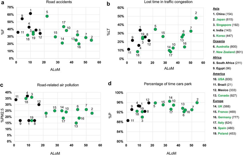
www.nature.com/scientificreports/
Figure 3. Comparison of fastest travel mode between PT and PCs for 17 cities (Supplementary Tables 2, 3 and
4). (a) Data points of the 17 cities for four contour maps, where, in referring to Fig. 2, TBEC (Transit Beats or is
Equal to Cars) is the sum of the blue and green areas (in k m2), CBT (Cars Beat Transit) is the pink area (in k m2),
with city number marked as a data point. The four figures are proportional to the line of equality with different
scales used for TBEC and CBT. (b) All data points of the four contour-map scenarios for (a) using the same
colors as for the (a) data points.
Figure 3 depicts this comparison for the 17 cities selected, using three acronyms relating to travel times: CBT,
cars are better (faster) than transit, or Cars Beat Transit; TBC, transit is better than cars, or Transit Beats Cars;
and TBEC, transit is better than or equal to cars, or Transit Beats or is Equal to Cars. The four figures in Fig. 3
correspond to the line of equality.
Supplementary Table 4 shows the results for the 17 cities, for four contour maps of travel times from city cent-
ers to each selected zone. The contour map shows T minutes, T = 30, 45, 60, 90, representing how far one can drive
by PT or PC in a maximum of T minutes, in all travel directions during PM peak period from a selected city’s
center point. The 17 cities and four contour maps generated 68 different scenarios. Figure 2a for the Lower Man-
hattan zone of New York, and Fig. 2b for the Guomao zone of Beijing show where TBC, CBT and TBEC apply. PC
and PT travel times are considered equal if their difference is less than 5%. Using 30-min contour maps, Fig. 2c
shows examples of two cities (Chicago and Tokyo) with good PT, and two cities (Sydney and Singapore) with poor
Scientific Reports | (2021) 11:14597 | https://doi.org/10.1038/s41598-021-93741-4 5
Vol.:(0123456789)
www.nature.com/scientificreports/
PT. For km2, TBEC, TBC, CBT values are 124, 103, 3 and 129, 90, 5 for Chicago and Tokyo, respectively, and 61,
17, 25 and 32, 9, 20 for Singapore and Sydney, respectively. The initial point of departure in each city was in the
Randolph/Wabash vicinity in Chicago; the Tokyo train station; Westfield, Sydney; and Nex Mall in Singapore.
However, TBC (transit beats cars), TBEC (transit beats or is equal to cars), and CBT (cars beat transit) take
more than travel time into account37–39. PT route preferences also depend on other attributes including quality
of service, fares, accessibility, connectivity and journey distances40. Travelers strive for personalized mobility22,41
with the option of changing the relative value of TBC and CBT attributes at any time during the day. PT will
prevail over PC as a conscious decision if the public will consider it a better fit for its personalized mobility needs.
Travel time, however, is a critical attribute, c urrently39 and for the future42, in paving the way to considering
other attributes.
The methodology behind Figs. 2 and 3, using ArcGIS 10.3.1, is based on the Dijkstra, Prim and Kruskal
algorithms for traversing a street network using real time travel speed (Supplementary Fig. 1). Geological street
maps are used for network input. The polygons are generated using a triangular irregular network (TIN) format.
See “Method” of this section for more information. Finally, Fig. 3a illustrates the data points for the 17 cities,
including listing them by their numbers for each of the four contour maps. Figure 3b sums up the four figures
of Fig. 3a. Thus, areas in which the PCs are faster on the average than PT, CBT (km2) > TBEC (km2), were only
found for four scenarios: Shanghai for T = 30, Sydney for T = 60, 90, and Copenhagen for T = 90. Overall, PT is
superior or equivalent to PCs, entailing less travel time in 94% of the scenarios tested. This represents a signifi-
cant new finding.
Method. The objective of this part of the paper is to design a methodology to make global comparisons
between average urban travel times for PT and PCs. Data characteristics for Fig. 2 appear in Supplementary
Tables 1 and 2, with input and sources of data in Supplementary Table 9. The purpose of Figs. 2 and 3 is to exam-
ine which mode of travel is faster, PCs or PT, in the 17 world cities chosen. Four radiuses of travel times from
a city center were selected: 30, 45, 60 and 90 min using real data from the street network and travel speed from
5:00 to 6:00 p.m. The methodology for attaining the results in Figs. 2 and 3 is based on constructed procedures of
ArcGIS 10.3.1, depicted conceptually in Supplementary Fig. 1; the results are shown in Supplementary Table 4.
Basically, two network layers of the PT and PCs are analyzed.
Geologic street maps such as Google Maps, OpenStreetMap, Baidu Maps and NAVTEQ are input as nodes
and links, and the Dijkstra, Prim and Kruskal shortest path algorithms create the minimum time-based spanning
trees from the selected city’s starting point. All points that are less than or equal to the designated radius travel
time are saved for creating the contour map area.
The shortest path routing in terms of travel time is the base of comparison as is shown by Supplementary
Fig. 1. For the PCs, different, real observed speeds are used per segment of roadway between two junctions. For
the PT, the observed data refer to the timetables and speeds of the available PT travel modes for each end point
including the possibility of using more than one PT mode through making transfers. Thereafter, the minimum
travel time across all PT modes is selected for comparison with the same for a PC.
Accordingly, for the calculation of PT travel time, all PT routes are examined including bus, metro, rail, and
passenger ferry with transfer possibilities across the PT travel modes. Walking time to and from PT stops is based
on an average of 5 km/h walking speed. Transfer times, practically speaking, are calculated based on artificial
links created between the arrival point of one PT line and the departure point of the other PT line using the aver-
age walking speed, where the two PT lines can be of same or different travel mode. The waiting time is derived
from the frequency of each PT line based on its timetable assuming that it is half of the headway between two
consecutive PT vehicles. The headway is the inverse of the frequency. The use of real data makes it unnecessary
to use approximation modelling such as transit assignment models. The complete sources of the input data for
ArcGIS 10.3.1 appear in Supplementary Table 9.
An example of a foreseeable future scenario
Description and results. Following the global outlook for enormous traffic-damage problems, and the
significant (94%) advantage of PT over PCs, we can present an example of potential, sustainable urban mobility
as a foreseeable conclusion.
Thus, an identical, hypothetical, future scenario for all of the 17 cities and its implications is examined in order
to derive the number of automated vehicles expected to run in peak hours on the main roads. In constructing this
scenario, known notions and research studies on automated vehicles were considered42–44. This future scenario
is shown schematically in Fig. 4, where Zone A is defined as a residential zone and point B is defined as a real,
central shopping point in the canter of each city. The assumption is that a demand, uniformly distributed, of
1000 PCs, each with single person occupancy, is traveling from A to B between 3:00 and 5:00 p.m., using real PC
travel time for each city dependent on traffic conditions and road infrastructure. This future scenario exercise
examines the benefits and results of shifting the 1000 individuals, driving from A to B using 1000 ordinary PCs,
to automated PT vehicles.
As a basis for comparison, travel times from A1 (a central point of A for each of the 17 cities) to B are similar
at approximately 30 min, with approximately 20 min travel times in the absence of traffic congestion. Figure 4
assumes automated vehicles, not privately owned, hence considered as PT service, yet the infrastructure is
unchanged. Each of the 1000 persons has two choices: (1) to travel from home in A to B using individual auto-
mated PT vehicle (IAPTV), or (2) to travel from home (suggested that this be without charge) by individual
automated vehicle of local PT service (IAV-PT) to A1 and transfer to shared automated PT vehicle (APTV) that
will stop at B.
Scientific Reports | (2021) 11:14597 | https://doi.org/10.1038/s41598-021-93741-4 6
Vol:.(1234567890)www.nature.com/scientificreports/
Figure 4. A schematic description of the elements involved with the future mobility scenario. It shows that
Zone A is comprised of eight TIN sub-areas for individual automated vehicles of local PT service (IAV-
PTs), with its eight starting points. However, in this scheme, there are only five starting points for individual
automated PT vehicles (IAPTVs) located in five (out of eight) of the IAV-PT starting points. The requests for
travel are represented by Ri2 and Ri3 for using IAPTV and IAV-PT, respectively, and there is a measuring point
between A1 and B to count the number of shared, automated PT vehicles (APTVs) and IAPTVs compared with
the ordinary 1000 PCs.
The methodology developed is based on newly constructed procedures of ArcGIS 10.3.1 shown in Supple-
mentary Fig. 2. In ArcGIS 10.3.1, the shortest path routing (SPR) algorithms are used to create the triangulated
irregular network (TIN) area reachable by the maximum time criterion for the movements of IAPTVs and IAV-
PTs within zone A, and for APTVs and IAPTVs between A1 and B in both directions. Zone A contains eight
TIN sub-areas, SPR-based, with eight starting points for IAV-PTs, but with only five starting points for IAPTVs
without showing their TIN sub-areas. An illustrative example is shown in Fig. 4 where a specific IAPTV, with its
starting point at A1, is assigned to pick up the R32 request, and a specific IAV-PT is assigned to pick up R13, drop
it off at A1, and then, to handle the R23 request without returning to its starting point. In addition, Fig. 4 shows
the location of measuring the percent, considering 1000 PCs, of APTVs and IAPTVs for comparing it with the
ordinary situation of each of the 17 cities.
An initial departure location for each person is randomly assigned within A, with maximum eight-minute
wait times, and maximum eight-minute ride times by IAV-PTs. APTV and IAPTV speed are assumed to be
identical to the speed of a current bus route in a priority lane. APTVs and IAPTVs return to A after completing
their trips to B to transport more individuals. Figure 5 shows proportional relations between the percentage of
persons using choice (1), and those using choice (2). The methodology related to Fig. 5 appears in “Method” of
this section and Supplementary Fig. 2 using ArcGIS 10.3.1. In Fig. 5, there are three cases: [%APTVs, %IAT-
PVs] = [100, 0], [50, 50] and [0, 100] indicating the percentage of people using each of these two modes of travel.
Two more cases of [75, 25] and [25, 75] are shown in Supplementary Table 7. The seat occupancy and capacity
of an APTV is 20. The IAPTV and IAV-PT can take individuals, groups, a family or other defined group such as
friends; however, in this exercise each of these two travel modes takes only one person. The fare for IAPTV will
be higher than for a shared APTV. The results of the percentage of automated vehicles on the main road between
A and B, out of the 1000 ordinary PCs, appear at the end of each bar.
It is interesting to observe, in this simple exercise, that with only APTVs, the number of vehicles running on
the main road between A to B (Fig. 4) will be 3% of the current number of PCs. On the average, this 3% rises to
30% and 58% for the [50, 50] and [0, 100] cases, respectively. The potential reduction in the number of vehicles
following their automation corresponds well with the notion that less is more. Only the use of PT vehicles has a
high chance45,46 of reducing the number of vehicles, and thereby contributing to diminishing the negative effects
of road traffic.
Method. The objective of this part is to produce and describe a methodology for global analysis of a future,
automated scenario of urban mobility and the expected number of peak-hour vehicles to be operating on the
main roads. The schematic sketch of the future scenario examined, appears in Fig. 4 with its 17 city data for A,
Scientific Reports | (2021) 11:14597 | https://doi.org/10.1038/s41598-021-93741-4 7
Vol.:(0123456789)www.nature.com/scientificreports/
Figure 5. Reduction expected in the number of vehicles based on a future scenario (Fig. 4 and Supplementary
Table 6). There are three types of automated vehicles represented: IAPTV, local service IAV-PT, and a shared
APTV for three cases: [%APTVs, %IATPVs] = [100, 0], [50, 50] and [0, 100]. The percent at the end of each bar
shows the percentage of vehicles on the main road between A and B out of the 1000 ordinary PCs, i.e., without
IAV-PTs.
A1, B shown in Supplementary Table 5. This future scenario exercise investigates the results of a shift of 1000
individuals, going from A to B by 1000 ordinary PCs with single person occupancy, to automated PT vehicles.
The methodology for simulating the three layers of APTVs (automated PT vehicles), IAPTVs (individual auto-
mated PT vehicles) and IAV-PTs (individual automated vehicles of local PT service) is conceptually depicted in
Supplementary Fig. 2. The shortest path routing (SPR) procedures based on Dijkstra, Prim and Kruskal algo-
rithms are used by ArcGIS 10.3.1 to create the triangulated irregular network (TIN) area reachable by the maxi-
mum time criterion for the movements of IAPTVs and IAV-PTs within zone A, and for APTVs and IAPTVs
from A1 to B and vice versa. Real time traffic data from the 17 cities are used (Supplementary Table 9) to select
the A areas and B points to provide a basis of comparison for travel times of approximately 30 min from A to B.
For the same scenario, let k represent PT travel mode, where k = 1,2,3 applies to APTVs, IAPTVs, and IAV-
PTs, respectively. Let SPRk (u,v) be SPR (shortest path routing) from u to v using travel mode(s) k, k = 1,2,3; and
let Rrk be a travel request made at the point of origin of the PC, r, r = 1,2,…1000, for travel mode k, k = 2,3, where
all origins are uniformly distributed within A, but their travel requests are made randomly. There are a total of
1000 riding requests between A and B using either choice (1) to travel from home in A to B using IAPTV, or
choice (2) to travel from home to A1 using IAV-PT, and from A1 to B using APTV, between 3:00 and 5:00 p.m.
in zone A of each city. It is assumed that by using choice (1), IAPTVs are moving to B via A1, and the same
applies for the return trip from B to A1. This allows for the use of ArcGIS for this simulated scenario, partially
integrated with the APTV movements between A1 and B. Stated in other terms, the pickup for a travel request
at r, Rr2 will traverse SPR2(r,A1) and SPR2(A1,B). On the return trip, it will traverse SPR2(B,A1) and SPR2(A1,q),
where q can either be an assigned IAPTV starting point or the location of a new request Rq2.
The assigned IAPTV starting locations and the number of them depend on four parameters: (a) the assumed
number of requests (of 1000) for k = 2; (b) average round trip time, i.e., r–A1–B–A1–q using the aforementioned
interpretation; (c) maximum pickup time criterion needed to create the TIN area by ArcGIS; and (d) to overlap
with an existing (if any) IAV-PT starting location near the center of the TIN area. This is derived from an admin-
practical perspective. These assigned locations in the 17 A zones were found iteratively in a manner that follows
the concept of gradient-descent47 in its simulation of input of the four parameters. The main constraint imposed
by this procedure is in assuring that the travel time, i.e., r–A1–B, is less than that of an average PC r–B travel time.
Individuals who choose (2) will use a transfer between IAV-PT (suggested to be a free ride) and APTV at A1.
Thus, their travel time from r to B will involve four time elements: waiting time at r following Rr3, travel time for
SPR3(r,A1), waiting time for an APTV departure, and travel time for SPR1(A1,B). The IAV-PTs will also take a
returning individual from A1 back to the individual’s assumed home at r. The selection of the starting points of
IAV-PTs, and the number of them, depend on three parameters: (a) the assumed number of requests (of 1000) for
k = 1, (b) maximum pickup time following a request, and (c) maximum travel time to A1. The selected starting
locations of the 17 A zones, similar to those of the IAPTVs, were found by an iteration process using simulation
with an input of the three parameters. The principal constraint in this process is accommodating the r–A1–B
travel time so that it will be less than for an ordinary PC considering all four of the process’s time elements.
Certainly, these iterative IAPTV and IAV-PT procedures, for this simple future scenario, beg further elaboration.
Scientific Reports | (2021) 11:14597 | https://doi.org/10.1038/s41598-021-93741-4 8
Vol:.(1234567890)www.nature.com/scientificreports/
Finally, this analysis determines the required number of APTVs, IAPTVs, and IAV-PTs shown in Fig. 5, and
in Supplementary Tables 6 and 7. This also implies the number of APTVs and IAPTVs vehicles running during
the two hours on the A–B segment. This is interpreted as the percent of automated PT vehicles of 1000 ordinary
PCs, as shown in Fig. 5 and cited in Fig. 4. The number of required APTVs is the maximum number of departures
during a time window of the round trip time (A1–B–A1)48,49. This maximum number of departures is checked
throughout the total set of departures simulated over the two hours using the following process: individual pas-
sengers arriving randomly at A1 by IAV-PTs and create a departure of an APTV if either the 20-seat occupancy
is full, or if the APTV wait time reaches its maximum time. The number of APTV users is given, as well as the
number of IAPTV users, and both equal 1000.
The number of required IAPTVs is determined by simulating roundtrip travel time between two travel
requests, Rp2 and Rq2 , where Rq2 is the first request, feasible to accommodate, after a completion of a roundtrip
to B. The implications are that an IAPTV* picks up the individual behind Rp2 who traverses p–A1–B–A1–Sl2 ,
where Sl2 is its starting location at A, k = 2, and traverses Sl2–q if the q location is within the assigned TIN area of
IAPTV*, and there is no other IAPTV that can reach q before IAPTV*. This simulation process complies with the
constraint of maximum pickup time from making the random travel request for k = 2. The number of required
IAV-PTs is also determined by simulation, given the number of random requests in the two hours for APTVs,
and the starting locations Sl3 for each TIN area selected for IAV-PTs. In this simulation-based procedure, an
IAV-PT, after a passenger disembarks at A1, can either traverse its Sl3 or move directly from A1 to a new travel
request, as is shown by Fig. 4.
Contributions and discussion
The contributions of this work are the findings of (1) the magnitude of the global, urban superiority of PT vehicles
over PCs (94%), (2) the magnitude of the global picture, and types of road traffic damages, (3) the prospects for
reducing the number of vehicles in urban areas using automation by approximately two-thirds, and (4) the unique
construction of this three-part study that streamlines into the discussion and conclusions of the overall work.
The first three contributions are an assemblage of new concepts and data analyses that have not heretofore been
considered in this way. These contributions are the fundamental input for the following discussion and vision.
The limitations of the study are prescribed by the attempt to cover the big picture as required for drawing
conclusions about policy trends, diminishing possibilities for referring to possible fluctuations of data, and its
sensitivity analysis. Thus, the methodologies developed for attaining the contour maps and creating a future
mobility scenario (Supplementary Figs. 1 and 2) do not include stochastic optimization with consideration of
randomness.
With the current COVID-19 pandemic climacteric, there is a window of opportunity for governments pro-
actively find ways to reduce progressively increasing road traffic damages with the urban mobility of the future.
This presumption is integral to this paper from the introduction through to its conclusions. In the ordinary
flow of society and social lives, conservative attitudes natural to people, feeling safe in their familiar routines,
inhibit change in our best interests. In the context of this work, that refers to eliminating private cars as a means
of transportation.
Colossal road traffic damages (for 19-countries) are shown globally and contrary to sustainability, using four
traffic-related considerations: road-accident fatalities as responsible for 35.6% of all deaths from accidents; time
lost in traffic congestion as 22.5% of total commuting time; 14.4% of total risk PM2.5 coming from road traffic;
and 94.7% of the time that PCs spend parked indicative of their highly inefficient use.
Part of the misunderstanding regarding future mobility has its source in the vast amount of emerging ter-
minologies. PT can be perceived as an umbrella over all non-PCs, including those of transportation network
companies (TNCs)5,50 and mobility-as-a-service (MaaS), as well as transportation of goods51. Currently, most
future mobility news is about technological advances, along with research and modelling of AVs in consid-
eration of operational and economic issues52,53, human and societal perspectives1–3,6,19,38,44,54, and government
interference43,55. However, while technological progress will continue, the most dramatic, anticipated change
will be the cessation of driving PCs. The question is how to reach that point wisely.
Driving practices should change3, and be perceived, perhaps, like the process of quitting smoking56. It involves
changing people’s habits18 and confronting a sort of addiction to driving19. In a study of applied psychology57
it is shown that people often do not behave in a manner corresponding to their intentions because of various
difficulties and/or temptations. Schwarzer57 suggests the use of self‐efficacy and strategic planning in under-
standing the inconsistency between intention and behavior. This angle seems to be useful for any habit (not only
health-compromising behavior). Thus, the intention to use AVs is not easily implemented because of health- and
habit-compromising behaviors.
One tactic to reduce PC driving is to provide incentives complemented by clearly demonstrating that transit
is better than cars for individuals and society. This should be comprehended by individuals and groups as a
choice and not as a stipulated measure. Additionally, the implications of PC disappearance including the fate
of PC vehicles with the discontinuation of their use and a range of employment ramifications require attention.
Vision and concluding remarks
The preferred choice of using public transit over cars bears potential for the realization of sustainable, future,
urban mobility. Figure 6, as a vision, shows an appealing future concept for urban mobility without PCs, based on
globalization, personalization, prioritization, and standardization (GPPS) with special standardization require-
ments. Globalization is for reciprocal action between urban and national economies21; personalization is for
riding preference requests using two-way apps22,41; prioritization is for emergency transport, elderly people, VIP
with higher service classes23, etc. and standardization is for maximizing compatibility of connecting any two PT
Scientific Reports | (2021) 11:14597 | https://doi.org/10.1038/s41598-021-93741-4 9
Vol.:(0123456789)www.nature.com/scientificreports/
Figure 6. A vision of PT-based seamless urban future mobility. This is a schematic illustration of a feasible
urban scenario allowing vehicles to connect to each other physically for smooth transfer of travelers, based on
GPPS. Seamless connections of nine vehicles are represented: (1) a longitudinal connection between IAPTV
(individual automated PT vehicle) and a small APTV (automated PT vehicle), (2) a lateral connection between
two small APTVs, (3) a longitudinal connection between small and large APTVs, (4) a lateral connection
between high speed rail and a small APTV, (5) a lateral connection between city and intercity rail, (6) a
longitudinal connection between a vertical/diagonal elevator and a small APTV, (7) a longitudinal connection
between a horizontal and vertical elevator and a small APTV, (8) a IAPTV journey outside city region, and (9)
the flexibility of each APTV to carry goods and freight.
vehicles24. By analogy, standardization is unlike the lack of a universal electric plug because of various countries’
preferences for developing their own. One important feature in making PT better than cars is to combine its
seamless mobility25,48 with travelers’ p
references22. PT travelers are likely to have preferences depending on dif-
ferent attributes such as travel time, comfort, fares, accessibility, and connectivity. These can vary, for instance,
by time of day, mood, schedule to follow, family considerations, etc. Accordingly, a combined system of seamless
mobility with human preferences can be based on a well-designed smartphone application interacting with the
PT operator in terms of sending preferences, receiving tailored information, and optimally adjusting system
operation and synchronization48.
Scientific Reports | (2021) 11:14597 | https://doi.org/10.1038/s41598-021-93741-4 10
Vol:.(1234567890)www.nature.com/scientificreports/
The seamless connections shown by Fig. 6, based on GPPS, demonstrate a future automated transit system
centrally synchronized to meet people’s best real time preference-based requests. It illustrates a mobility system
moving horizontally and vertically, and possibly diagonally. The synchronized, seamless connections, between
and within IAPTVs (individual automated PT vehicles) and APTVs (automated PT vehicles), can be made either
laterally (connections 2, 4 and 5 in Fig. 6) or longitudinally (connections 1, 3, 6 and 7). Figure 6 includes an
example (number 8) of a journey outside the urban area where further coordinated connections can take place58.
Finally, it provides one example (number 9) of the use of an APTV to deliver goods/freight that either belong
to the travelers or are an additional service taking advantage of the automated system. Certainly, the logistics of
such an ideal and sustainable future mobility must be based on prudent algorithms, real time processing with
a strong backup, and securely protected procedures. It will also include optimal allocation of the location and
parking of idle, automated vehicles. These logistics will follow a period of gradual changes incorporated with
some new i deas59 for this term.
A perception of a future PT service similar to services of a supermarket is behind Fig. 6. By this conceptual-
ization, ordering food is analogous to IAPTVs, while visiting a supermarket and collecting merchandise from
a broad variety of choices is analogous to economy, premium, first class APTVs. Ultimately, this study aims to
trigger a process of rethinking the unclear course of future-mobility development, by being proactive and allow-
ing AVs only for standardized PT, using the present window of opportunity. With recent changes in perception
of social distance, resulting from the COVID-19 pandemic, this study should contribute to inevitable popular
and scholarly processes of rethinking concomitant with changing habits, behavior, and thinking paradigms, and
to accepting new, automated, healthier, improved means of urban mobility.
Received: 2 May 2021; Accepted: 22 June 2021
References
1. Hecht, J. Meeting people’s expectations. Nature 563, S141–S143 (2018).
2. Bonnefon, J.-F., Shariff, A. & Rahwan, I. The social dilemma of autonomous vehicles. Science 352, 1573–1576 (2016).
3. Haboucha, C. J., Ishaq, R. & Shiftan, Y. User preferences regarding autonomous vehicles. Transp. Res. C 78, 37–49 (2017).
4. Ceder, A. Urban mobility and public transport: Future perspectives and review. Int. J. Urban Sci. https://doi.org/10.1080/12265
934.2020.1799846 (2020).
5. Diao, M., Kong, H. & Zhao, J. Impacts of transportation network companies on urban mobility. Nat. Sustain. https://doi.org/10.
1038/s41893-020-00678-z (2021).
6. Hancock, P. A., Nourbakhsh, I. & Stewart, J. On the future of transportation in an era of automated and autonomous vehicles.
PNAS 116(16), 7684–7691 (2019).
7. Nunes, A., Reimer, B. & Coughkin, J. F. People must retain control of autonomous vehicles. Nature 556, 169–171 (2018).
8. Legacy, C., Ashmore, D., Scheurer, J., Stone, J. & Curtis, C. Planning the driverless city. Transp. Rev. 39, 84–102 (2019).
9. Greene, A. N. Horses at Work: Harnessing Power in Industrial America (Harvard University Press, 2008).
10. Geels, F. W. The dynamics of transitions in socio-technical systems: a multi-level analysis of the transition pathway from horse-
drawn carriages to automobiles (1860–1930). Tech. Anal. Strat. Mgmt. 17, 445–476 (2005).
11. Unger, N. et al. Attribution of climate forcing to economic sectors. Proc. Natl. Acad. Sci. 107, 3382–3387 (2010).
12. IPCC. Climate Change 2014: Mitigation of Climate Change (Cambridge University Press, 2015).
13. Inci, E. A review of the economics of parking. Econ. Trans. 4, 50–63 (2015).
14. Bhalla, K., et al. Transport for health: the global burden of disease from motorized road transport (English). Washington, D.C.:
World Bank Group. http://documents.worldbank.org/curated/en/984261468327002120/Transport-for-health-the-global-burden-
of-disease-from-motorized-road-transport (2014).
15. Staton, C. et al. Road traffic injury prevention initiatives: A systematic review and metasummary of effectiveness in low and mid-
dleincome countries. PLoS ONE 11, 1–15 (2016).
16. Sweet, M. Traffic congestion’s economic impacts: Evidence from US metropolitan regions. Urban Stud. 51, 2088–2110 (2014).
17. Karagulian, F. et al. Contributions to cities’ ambient particulate matter (PM): A systematic review of local source contributions at
global level. Atmos. Environ. 120, 475–483 (2015).
18. Wood, W., Tam, L. & Witt, M. G. Changing circumstances, disrupting habits. J. Pers. Soc. Psycho. 88, 918–933 (2005).
19. Wood, T. Our addiction to driving is costing lives, and more. Torontoist, citiscape. https://torontoist.com/2018/03/addiction-drivi
ng-costing-lives/ (2018).
20. James, P., Magee, L., Scerri, A. & Steger, M. Urban Sustainability in Theory and Practice: Circles of Sustainability (Routledge and
Earthscan, 2015).
21. Guttal, S. Globalisation. Dev. Pract. 17, 523–531 (2007).
22. Ceder, A. & Jiang, Y. Route guidance ranking procedures with human perception consideration for personalized public transport
service. Transp. Res. C https://doi.org/10.1016/j.trc.2020.102667 (2020).
23. Nellore, K. & Hancke, G. P. Traffic management for emergency vehicle priority based on visual sensing. Sensors 16, 1892 (2016).
24. Katsikeas, C. S., Samiee, S. & Theodosios, M. Strategy fit and performance consequences of international marketing standardiza-
tion. Strat. Mgmt. J. 27, 867–890 (2006).
25. Wolff, C., Heller, M., Corwin, S., Bansal, M. P. & Pankratz, D. Activating a Seamless Integrated Mobility System (SIMSystem):
Insights into leading global practices. https://www.weforum.org/reports/activating-a-seamless-integrated-mobility-system-simsy
stem-insights-into-leading-global-practices (World Economic Forum, 2020).
26. Global status report on road safety 2018. https://www.who.int/violence_injury_prevention/road_safety_status/2018/en/ (World
Health Organization, Geneva, 2018)
27. Leape, J. The London congestion charge. J. Econ. Perspect. 20, 157–176 (2006).
28. Kai Zhanga, K. & Battermanb, S. Air pollution and health risks due to vehicle traffic. Sci. Total Environ. 450–451, 307–316 (2013).
29. Schneider, B. Traffic’s mind-boggling economic toll. Bloomberg Citilab. https://www.citylab.com/transportation/2018/02/traffi cs-
mind-boggling-economic-toll/552488/ (2018).
30. Kheirbek, I., Haney, J., Douglas, S., Ito, K. & Matte, T. The contribution of motor vehicle emissions to ambient fine particulate
matter public health impacts in New York City: A health burden assessment. Environ. Health 15, 89–102 (2016).
31. Berntsen, T. & Fuglestvedt, J. Global temperature responses to current emissions from the transport sectors. PNAS 105(49),
19154–19159 (2008).
32. Rodrigue, J.-P., Comtois, C. & Slack, B. The Geography of Transport Systems 4th edn. (Routledge, 2017).
Scientific Reports | (2021) 11:14597 | https://doi.org/10.1038/s41598-021-93741-4 11
Vol.:(0123456789)www.nature.com/scientificreports/
33. Dey, P. P., Chandra, S. & Gangopadhaya, S. Speed distribution curves under mixed traffic conditions. J. Trans. Eng. 132, 475–481
(2006).
34. Mehar, A., Chandra, S. & Velmurugan, S. Speed and acceleration characteristics of different types of vehicles on multi-lane high-
ways. Euro. Trans. 55, 1–12 (2013).
35. Speed limit by country. ChartsBin.com , viewed 18 June 2019. http://chartsbin.com/view/41749 (2019).
36. Highway statistics 2016. https://www.fhwa.dot.gov/policyinformation/statistics/2016/vm1.cfm (U.S. Department of Transporta-
tion, Federal Highway Administration, 2016).
37. Kii, M. & Hanaoka, S. Comparison of sustainability between private and public transport considering urban structure. IATSS Res.
27(2), 6–15 (2003).
38. Steg, L. Can public transport compete with the private car?. IATSS Res. 27(2), 27–35 (2003).
39. Salonen, M. & Toivonen, T. Modelling travel time in urban networks: Comparable measures for private car and public transport.
J. Transp. Geogr. 31, 143–153 (2013).
40. Grison, E., Burkhardt, J. M. & Gyselinck, V. How do users choose their routes in public transport? The effect of individual profile
and contextual factors. Trans. Res. F 51, 24–37 (2017).
41. Lathia, N., Smith, C., Froehlich, J. & Capra, L. Individuals among commuters: Building personalised transport information services
from fare collection systems. Pervasive Mob. Comput. 9, 643–664 (2013).
42. Singleton, P. E. Discussing the “positive utilities” of autonomous vehicles: Will travelers really use their time productively?. Transp.
Rev. 39, 50–65 (2019).
43. Straub, E. R. & Schaefer, E. It takes two to tango: Automated vehicles and human beings do the dance of driving—Four social
considerations for policy. Transp. Res. A 122, 173–183 (2019).
44. Herb, M., Xiao, Y., Circella, G., Mokhtarian, P. L. & Walker, J. L. Projecting travelers into a world of self-driving vehicles: Estimating
travel behavior implications via a naturalistic experiment. Transportation 45, 1671–1685 (2018).
45. Chen, T. D., Kockelman, K. M. & Hanna, J. P. Operations of a shared, autonomous, electric vehicle fleet: Implications of vehicle
and charging infrastructure decisions. Trans. Res. A 94, 243–254 (2016).
46. Vazifeh, M. M., Santi, P., Resta, G., Strogatz, S. H. & Ratti, C. Addressing the minimum fleet problem in on-demand urban mobility.
Nature 557, 534–553 (2018).
47. Ruder, S. An overview of gradient descent optimization algorithms. arXiv:1609.04747 [cs.LG]. https://arxiv.org/pdf/1609.04747.
pdf (2017).
48. Ceder, A. Public Transit Planning and Operation 2nd edn. (CRC Press, 2016).
49. Salzborn, F. J. M. Optimum bus scheduling. Trans. Sci. 6, 137–148 (1972).
50. Feigon, S. & Murphy, C. Broadening understanding of the interplay between public transit, shared mobility and personal auto-
mobiles, TCRP Research Report 195. https://doi.org/10.17226/24996 (The National Academies Press, Washington, DC, 2018).
51. Bechtsis, D., Tsolakis, N., Vlachos, D. & Srai, J. S. Intelligent autonomous vehicles in digital supply chain: A framework for integrat-
ing innovations toward sustainable value networks. J. Clean. Prod. 181, 60–71 (2018).
52. Wang, H. et al. Crash mitigation in motion planning for autonomous vehicles. IEEE Trans. Intell. Transp. Syst. 20(9), 3313–3323
(2019).
53. Li, B. et al. Estimation of regional economic development indicator from transportation network analytics. Sci. Rep. 10, 2647.
https://doi.org/10.1038/s41598-020-59505-2 (2020).
54. Shariff, A., Bonnefon, J.-F. & Rahwan, I. Psychological roadblocks to the adaption of self-driving vehicles. Nat. Hum. Behav. 1,
694–696 (2017).
55. Cohen, T. & Cavoli, C. Automated vehicles: Exploring possible consequences of government (non)intervention for congestion
and accessibility. Transp. Rev. 39, 125–151 (2019).
56. McCarthy, N. U.S. smoking rate falls to record low. Topics-Smoking. https://www.statista.com/chart/14879/us-smoking-rate-falls-
to-record-low/ (Statista, 2018).
57. Schwarzer, R. Modeling health behavior change: How to predict and modify the adoption and maintenance of health behaviors.
Appl. Psychol. 57, 1–29 (2008).
58. Hansson, J., Pettersson, F., Svensson, H. & Wretstrand, A. Preferences in regional public transport: A literature review. Eur. Transp.
Res. Rev. 11, 38 (2019).
59. Bagloee, S. A., Ceder, A., Sarvi, M. & Asadi, M. Is it time to go for no-car zone policies? Braess paradox detection. Transp. Res. A
121, 251–264 (2019).
Acknowledgements
Thanks are due to J. Song for continuous help with data for the 17 cities; Z. Cao for assistance with data for
the 19 countries; T. Liu for early discussions, and to the Korean Transport Institute (KOTI) for stimulating my
interest in the subject.
Author contributions
A.C. conceived the work, developed its methodologies, designed and conducted the analyses, created the figures,
tables and artwork, and wrote the manuscript.
Competing interests
The author declares no competing interests.
Additional information
Supplementary Information The online version contains supplementary material available at https://doi.org/
10.1038/s41598-021-93741-4.
Correspondence and requests for materials should be addressed to A.C.
Reprints and permissions information is available at www.nature.com/reprints.
Publisher’s note Springer Nature remains neutral with regard to jurisdictional claims in published maps and
institutional affiliations.
Scientific Reports | (2021) 11:14597 | https://doi.org/10.1038/s41598-021-93741-4 12
Vol:.(1234567890)You can also read