The completed SDSS-IV extended Baryon Oscillation Spectroscopic Survey: large-scale structure catalogues and measurement of the isotropic BAO ...
←
→
Page content transcription
If your browser does not render page correctly, please read the page content below
MNRAS 500, 3254–3274 (2021)                                                                                                 doi:10.1093/mnras/staa3336
Advance Access publication 2020 October 28

The completed SDSS-IV extended Baryon Oscillation Spectroscopic
Survey: large-scale structure catalogues and measurement of the isotropic
BAO between redshift 0.6 and 1.1 for the Emission Line Galaxy Sample
Anand Raichoor,1‹ Arnaud de Mattia,2 Ashley J. Ross ,3 Cheng Zhao ,1 Shadab Alam,4
Santiago Avila,5,6 Julian Bautista ,7 Jonathan Brinkmann,8 Joel R. Brownstein ,9 Etienne Burtin,2
Michael J. Chapman,10,11 Chia-Hsun Chuang ,12 Johan Comparat,13 Kyle S. Dawson,9 Arjun Dey,14
Hélion du Mas des Bourboux,9 Jack Elvin-Poole,3 Violeta Gonzalez-Perez ,7,15 Claudio Gorgoni,1

                                                                                                                                                           Downloaded from https://academic.oup.com/mnras/article/500/3/3254/5942664 by guest on 22 February 2021
Jean-Paul Kneib,1,16 Hui Kong ,3 Dustin Lang,11,17 John Moustakas,18 Adam D. Myers,19
Eva-Maria Müller,20 Seshadri Nadathur ,7 Jeffrey A. Newman,21 Will J. Percival,10,11,17
Mehdi Rezaie ,22 Graziano Rossi,23 Vanina Ruhlmann-Kleider,2 David J. Schlegel,24
Donald P. Schneider,25,26 Hee-Jong Seo ,22 Amélie Tamone,1 Jeremy L. Tinker ,27 Rita Tojeiro ,28
M. Vivek,25,29 Christophe Yèche2,24 and Gong-Bo Zhao7,30,31
Affiliations are listed at the end of the paper

Accepted 2020 October 17. Received 2020 October 16; in original form 2020 May 19

ABSTRACT
We present the Emission Line Galaxy (ELG) sample of the extended Baryon Oscillation Spectroscopic Survey from the Sloan
Digital Sky Survey IV Data Release 16. We describe the observations and redshift measurement for the 269 243 observed
ELG spectra, and then present the large-scale structure catalogues, used for the cosmological analysis, and made of 173 736
reliable spectroscopic redshifts between 0.6 and 1.1. We perform a spherically averaged baryon acoustic oscillations (BAO)
measurement in configuration space, with density field reconstruction: the data two-point correlation function shows a feature
consistent with that of the BAO, the BAO model being only weakly preferred over a model without BAO (χ 2 < 1). Fitting
a model constrained to have a BAO feature provides a 3.2 per cent measurement of the spherically averaged BAO distance
DV (zeff )/rdrag = 18.23 ± 0.58 at the effective redshift zeff = 0.845.
Key words: galaxies: distances and redshifts – dark energy – distance scale – large-scale structure of Universe – cosmology:
observations.

                                                                               from 45 000 Luminous Red Galaxies (LRGs, Eisenstein et al. 2001).
1 I N T RO D U C T I O N
                                                                               It was the first BAO detection along with the 2dF Galaxy Redshift
The acceleration of the expansion of the Universe discovered about             Survey (Colless et al. 2003; Cole et al. 2005). The BOSS survey
20 yr ago (Riess et al. 1998; Perlmutter et al. 1999) set a key milestone      (2008–2014, Dawson et al. 2013) from the SDSS-III (Eisenstein
in cosmology history: current observations can be accounted for                et al. 2011) then massively observed 1.5 million LRGs and 160 000
with the CDM standard model, but at the cost of introducing                   quasars (QSOs), leading to a state-of-the-art 1–2 per cent precision
a dark energy component, making up today ∼70 per cent of the                   measurement of the cosmological distance scale for redshifts z <
energy content of the Universe. Around the same time, the SDSS                 0.6 (Alam et al. 2017) and z = 2.5 (Delubac et al. 2015; Bautista
collaboration (York et al. 2000) initiated spectroscopic observations          et al. 2017). The Extended Baryon Oscillation Spectroscopic Survey
to study large-scale structures (LSSs), which allows one to constrain          (eBOSS, 2014–2020, Dawson et al. 2016) of the SDSS-IV (Blanton
the geometry of the Universe with the Baryonic Acoustic Oscillations           et al. 2017) observed nearly one million objects to complement
(BAO, Eisenstein & Hu 1998) and the growth of structures with                  the BOSS survey in the 0.6 < z < 2.2 redshift range. eBOSS
redshift space distortion (RSD, Kaiser 1987).                                  observed LRGs at 0.6 < z < 1.0 (Prakash et al. 2016), Emission Line
   Since then, the SDSS has become a key experiment for the BAO,               Galaxies at 0.6 < z < 1.1 (ELGs, Raichoor et al. 2017), and QSOs
one of the most powerful cosmological probes (see Weinberg et al.              at 0.9 < z < 3.5 (Myers et al. 2015; Palanque-Delabrouille et al.
2013, for a review). The SDSS first measured the distance-redshift             2016).
relation with 5 per cent precision at z = 0.35 (Eisenstein et al. 2005)           We present in this paper the eBOSS/ELG spectroscopic observa-
                                                                               tions from the final release from SDSS-IV eBOSS Data Release 16
                                                                               (DR16; Ahumada et al. 2020), along with the construction of the LSS
   E-mail: anand.raichoor@epfl.ch                                             catalogues, and the spherically averaged BAO measurement from

                                                                                                                                   C 2020 The Author(s)

                                                                            Published by Oxford University Press on behalf of Royal Astronomical Society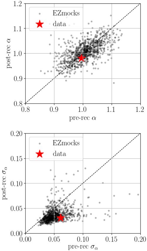
SDSS/eBOSS DR16 ELG LSS and isotropic BAO                                   3255
those. The LSS catalogues are also used in de Mattia et al. (2020) and       2 DATA
Tamone et al. (2020) to analyse the ELG anisotropic clustering. ELGs
                                                                             We describe in this section the target selection, the spectroscopic
are star-forming galaxies with strong emission lines – noticeably the
                                                                             observations, and the spectroscopic redshift (zspec ) estimation of the
[O II] doublet emitted at (λ3727, λ3729 Å), allowing a spectroscopic
                                                                             eBOSS/ELG sample.
redshift (zspec ) measurement in a reasonable amount of exposure
time, as there is no need to significantly detect the continuum. This
observational feature, combined with their abundance at z ∼ 0.5–
2 due to the high star formation density of the Universe then (e.g.          2.1 Imaging and target selection
Lilly et al. 1996; Madau, Pozzetti & Dickinson 1998; Madau &                 The ELG target selection is extensively described in Raichoor et al.
Dickinson 2014), makes them a promising tracer for LSSs surveys.             (2017) to which we refer the reader for more details.
The WiggleZ experiment (2006–2011, Drinkwater et al. 2010) was                  Targets are selected using the DECaLS part of the Legacy Imaging
the first ELG BAO survey. Now eBOSS paves the way for the next-              Surveys5 (Dey et al. 2019) grz photometry, which also provides
generation LSS surveys, which will heavily rely on the ELGs in the           the imaging for the DESI target selection. In detail, the DECaLS

                                                                                                                                                               Downloaded from https://academic.oup.com/mnras/article/500/3/3254/5942664 by guest on 22 February 2021
0.5  z  2 range, as PFS1 (Sugai et al. 2012; Takada et al. 2014),          program is a consistent processing of public imaging taken with the
DESI2 (DESI Collaboration 2016a,b), Euclid (Laureijs et al. 2011),           Dark Energy Camera (DECam Flaugher et al. 2015), mostly coming
and WFIRST 3 (Doré et al. 2018). Indeed, this eBOSS/ELG sample              from the DECaLS survey (co-PIs: A. Dey and D.J. Schlegel; NOAO
has already been used for several analyses, which strengthen our             Proposal # 2014B-0404) and the DES6 (PI: J. Frieman; NOAO
understanding of ELGs at z ∼ 1: exploring their physical content             Proposal # 2012B-0001). Comparat et al. (2016) and Raichoor et al.
(Gao et al. 2018; Huang et al. 2019), their dark matter haloes               (2016) demonstrated that DECaLS permits a better target selection
properties (Gonzalez-Perez et al. 2018; Guo et al. 2019; Gonzalez-           in terms of higher redshift and density than the SDSS imaging. The
Perez et al. 2020), and alternative methods to improve the removal           footprint is divided in two parts (see Fig. 1): ∼620 deg2 in the Fat
of systematics in their clustering (Kong et al. 2020; Rezaie et al.          Stripe 82 in the South Galactic Cap (SGC) at −43◦
3256        A. Raichoor et al.

                                                                                                                                                                 Downloaded from https://academic.oup.com/mnras/article/500/3/3254/5942664 by guest on 22 February 2021
Figure 1. Geometry of the ELG program. The NGC tiling is presented in the top panel: chunk eboss23 is at lower Dec. and chunk eboss25 at higher Dec.
The SGC tiling is presented in the bottom panel: chunk eboss21 is at R.A.0◦ . The colour-coding is the tiling completeness
(COMP BOSS), which represents the fraction of resolved fibres per sector (see Section 3.4). Additionally, we overlay some a posteriori angular veto masks,
which are detailed in Section 3.2: Mira star (light grey), DECam pointings with bad photometric calibration (dark grey), and two low-quality spectroscopic
plates (black). The regions without targets at R.A∼130◦ and Dec.∼20◦ correspond to the open cluster NGC 2632.

cuts for SGC:                                                                   divided in two chunks, eboss23 and eboss25. Observations are
                                                                                designed by defining the plate tiling (Blanton et al. 2003), which
21.825 < g < 22.825                                                  (1a)
                                                                                optimizes for each chunk the fraction of targets having a fibre
                                                                                for the budgeted number of plates. Fig. 1 shows the plate tiling,
− 0.068 × (r − z) + 0.457 < g − r < 0.112 × (r − z) + 0.773
                                                                                with the tiling completeness, defined as the fraction of resolved
                                                                     (1b)       targets (see Section 3.4, this corresponds to the COMP BOSS
                                                                                quantity in previous BOSS/eBOSS analysis). We note the narrow
0.218 × (g − r) + 0.571 < r − z < −0.555 × (g − r) + 1.901                      width (4◦ ) of the eboss21 chunk in the Dec. direction, which
                                                                     (1c)       is constrained by the available imaging. Given it is the order of
                                                                                the size of the BAO scale, this is likely not an optimal geometry,
and here the magnitude cuts for the NGC:
                                                                                but it is not a significant problem as the R.A. and radial directions
21.825 < g < 22.9                                                    (2a)       provide numerous ELG pairs at the BAO scale. Besides, this is fully
                                                                                accounted for in our analysis with our random catalogues (Section 3)
− 0.068 × (r − z) + 0.457 < g − r < 0.112 × (r − z) + 0.773                     and with the validation of the analysis with the mock catalogues (see
                                                                     (2b)       Sections 4 and 5). We report in Table 1 the details of the spectroscopic
                                                                                observations for each chunk and for the whole programme.
0.637 × (g − r) + 0.399 < r − z < −0.555 × (g − r) + 1.901.                        Details of the spectroscopic setup are presented in Raichoor et al.
                                                                                (2017). Each plate is observed with individual exposures of 15 min
                                                                     (2c)       until rSN2 > 22, where rSN2 is the median-squared signal-to-noise
It provides a list of 269 718 targets.                                          ratio (SN) in the red camera evaluated at the mountain. This is reached
                                                                                on average with 4.7 × 15 min exposures; the average SN on individual
                                                                                ELG spectra9 is ∼0.8. During the first month of operations (around
2.2 Spectroscopic observations                                                  half of the eboss21 chunk), observations were done with higher
The ELG spectroscopic observations are conducted with the BOSS                  rSN2 (∼40).
spectrograph (Smee et al. 2013) at the 2.5-m aperture Sloan Founda-                If one plate has to be unplugged before it reaches the minimum
tion Telescope at Apache Point Observatory in New Mexico (Gunn                  rSN2 , it is plugged again later and re-observed: as the fibres are
et al. 2006). The BOSS spectrographs resolution for 5950 Å< λ <                 not assigned to the same targets between the two pluggings, this
7850 Å, where the [O II] doublet lies for 0.6 < z < 1.1, is 1800 <              results in two PLATE-MJD reductions for the considered plate. This
R < 2500, which does not permit to clearly resolve the [O II] doublet           provides valuable independent, repeat observations for ELGs on that
(Comparat et al. 2013). 1000 objects are observed at once, with                 plate, which allows us to quantify the reliability of our redshift
1000 fibres plugged into a drilled plate, among which ∼850 are                  measurement (see Section 2.3).
assigned to ELGs. 305 plates have been allocated to the ELG program
and observations were undertaken between September 2016 and
February 2018 (57656 ≤ MJD ≤ 58171). Targeting was performed                    9 i.e. the average value of the idlspec2d SN    MEDIAN ALL quantity, which
on subsets of the full eBOSS/ELG area, called chunks: the SGC is                measures the median signal to noise per pixel across full spectrum in physical
divided in two chunks, eboss21 and eboss22, and the NGC is                      units of erg.s−1 .cm−2 .Å−1 ; see column (8) of Table 1.

MNRAS 500, 3254–3274 (2021)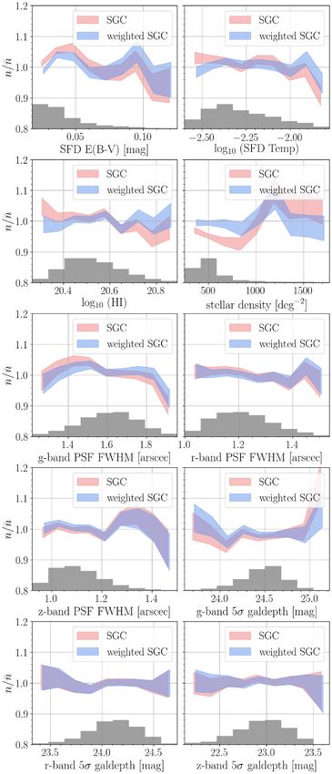
SDSS/eBOSS DR16 ELG LSS and isotropic BAO                                       3257
Table 1. Spectroscopic observations properties per chunk: (1): chunk name; (2): tiling area (deg2 ); (3): number of plates; (4): number of PLATE-MJD reductions;
(5): average observed time in minutes per PLATE-MJD; (6): average observed time in minutes included in the reduction per PLATE-MJD; (7): mean plate rSN2 ;
(8): mean SN per spectrum; (9): number of targets; (10): number of observed spectra; (11): number of spectra after removing duplicates; (12): number of targets
after applying the veto LSS masks; (13): number of star spectra after applying the veto LSS masks; (14): number of galaxy spectra after applying the veto LSS
masks; and (15): number of galaxy spectra after applying the veto LSS masks and with a reliable redshift.

(1)             (2)      (3)        (4)        (5)       (6)     (7)     (8)         (9)       (10)        (11)        (12)       (13)        (14)         (15)
                                    MJD         obs      kept                                              obs,uniq                           LSS,gal    LSS,gal
Chunk          Area     NPLATE     NPLATE      texp     texp    rSN2    SNspec       Ntarg       obs
                                                                                               Nspec      Nspec          LSS
                                                                                                                       Ntarg      LSS,star
                                                                                                                                 Nspec       Nspec      Nspec,reliable
              (deg2 )                         (min)    (min)

eboss21        171        46         46       122      100      28.7     0.99        40904     38992       38493       36314       333        33884       31200
eboss22        445       121        131        86       73      22.1     0.85       106897    111061      101954       79880       512        75585       69071
eboss23        377        87         92        70       60      25.4     0.82        76236     76250       71134       70935       544        65677       58648
eboss25        178        51         51        59       54      24.6     0.81        45141     42940       42863       42565       315        40141       36166
all           1170       305        320        82       70      24.0     0.84       269178    269243      254444      229694      1704       215287      195085

                                                                                                                                                                         Downloaded from https://academic.oup.com/mnras/article/500/3/3254/5942664 by guest on 22 February 2021
   Because of dead fibres or observational issues (e.g. incorrect plug-                     Following the eBOSS requirements (Dawson et al. 2016; Raichoor
ging of a fibre), some spectra are unusable. We identify those cases                     et al. 2017), redshift estimates should be precise (|v| < 300 km s−1 )
by using the ZWARNING quantity output by the redshift fitter (see                        and accurate (less than 1 per cent catastrophic redshifts, defined as
table 3 of Bolton et al. 2012): when one of the LITTLE COVERAGE,                         |v| > 1000 km s−1 ). To match these requirements, we define a
UNPLUGGED, BAD TARGET, or NODATA bits is turned on, we label                             redshift estimate reliable if the following criteria are satisfied:
the fibre as not valid, and as a consequence, we discard the spectrum
and consider that no spectroscopic observation has been taken.                           (ZWARNING == 0) and                                                     (3a)
   Overall, there are 14 799 repeat ELG spectra, or duplicates.
Duplicates happen for two reasons. First, when a PLATE has several                       (SN MEDIAN[i] > 0.5 or SN MEDIAN[z] > 0.5) and                          (3b)
MJD reductions: all ELGs on the plate will have as many zspec
measurements as MJD reductions. In that case, we consider as                             (zQ >= 1 or zCont >= 2.5).                                              (3c)
primary spectra all spectra coming from the MJD reduction with the                       In the following, we call a ‘failure’ a redshift measurement that does
higher plate SN, and as duplicates, the spectra from the other MJD                       not pass those equations, i.e. which is not considered as reliable. The
reductions. Secondly, in the plate overlap regions, any remaining                        first criterion (equation 3a) is based on the ZWARNING flag output
fibres are assigned to repeats: the fibre is then assigned to a target,                  by redrock (see Section 2.2) and ensures that the fitting did not
which already has a fibre assigned from another overlapping plate.                       encounter any problems. In particular, it assures that the coefficient in
In that case, we consider as primary the spectrum with a valid fibre                     front of the best-fitting archetype spectrum is positive, meaning that
and with the highest χ 2 difference between the best-fitting solution                    the best-fitting template is physically motivated (see Ross et al. 2020).
and the second best-fitting solution.                                                    The second criterion (equation 3b) ensures a minimum SN in the red
                                                                                         part of the spectrum, where the [O II] line is expected to be observed
                                                                                         at z ∼ 1.11 The third criterion (equation 3c) reduces the fraction of
2.3 Spectroscopic redshift estimation: redrock
                                                                                         catastrophic redshifts; it is based on the {zQ, zCont} a posteriori
The results presented in this paper use version v5 13 0 of the                           flags (see Comparat et al. 2016; Raichoor et al. 2017), which quantify
idlspec2d data reduction pipeline to extract and flux-calibrate                          the emission lines and continuum level of information. The impact of
the ELG 1D spectra from the raw 2D spectroscopic images (Bolton                          each cut, along with the improvement with respect to idlspec1d,
et al. 2012; Ahumada et al. 2020). As stated in Raichoor et al. (2017),                  is shown in Table 2 (the catastrophic rate is estimated with repeat
the BOSS/eBOSS redshift fitter, idlspec1d, is not optimized for                          observations, as described further in this section). One can see the
ELGs, as it has been designed for bright LRGs. Therefore, we used                        significant improvement brought by redrock with respect to the
for the 1D spectrum analysis redrock,10 the DESI redshift fitter,                        reliability criterion presented in Raichoor et al. (2017), based on
which provides more reliable redshifts.                                                  idlspec1d: it allows us to include in our cosmological 0.6 <
    We present here a summary of the redrock principle; we refer                         zspec < 1.1 sample more reliable redshifts (80.7 per cent versus
the reader to Ross et al. (2020) for more details. redrock tem-                          74.0 per cent, for a Poissonian fluctuation of ∼0.3 per cent), with
plates, labelled archetypes, are the most representative (simulated)                     a lower fraction of catastrophic rate (0.3 per cent versus 0.5 per cent,
physical spectra of DESI galaxies, QSOs, and stars. redrock                              for a Poissonian fluctuation of ∼0.06 per cent). Those improvements
fitting procedure includes two steps. In the first step, it finds the χ 2                are significant, well above the Poissonian noise fluctuations. We
minima using principal-component analysis (PCA) templates, based                         validate our reliability criteria with two approaches, visual inspection
on DESI archetypes. As the best-fitting PCA spectra can be non-                          and repeat observations.
physical, for each minimum vicinity, redrock then recomputes                                Three plates have been visually inspected, one from the
the χ 2 with archetypes. This approach ensures that the best-fitting                     eBOSS/ELG program (PLATE-MJD = 9236-57685) and two from
solution corresponds to a physical, meaningful, spectrum.                                pilot ELG programs (PLATE-MJD = 6931-56388 and 8123-56931).
                                                                                         We restrict here to the ∼1900 ELGs with 0.6 < zspec < 1.1 that
                                                                                         passed our reliable criteria listed in equations (3a), (3b), and (3c).
10 https://github.com/desihub/redrock;       we used a customed version of the           The inspector assigns a visual redshift and one of the following
tagged version 0.14.0, where we do not use the ANDMASK masking, as it
unnecessarily removes pixels close to sky emission lines from the fit, hence
creating artificial drops in the redshift density n(z), where the [O II] doublet         11 SN MEDIAN[i,z] is the median SN for all good pixels from the spectrum

falls close to sky lines; that version is internally labelled v5 13 0 no andmask.        corresponding to the i- and z-bands.

                                                                                                                               MNRAS 500, 3254–3274 (2021)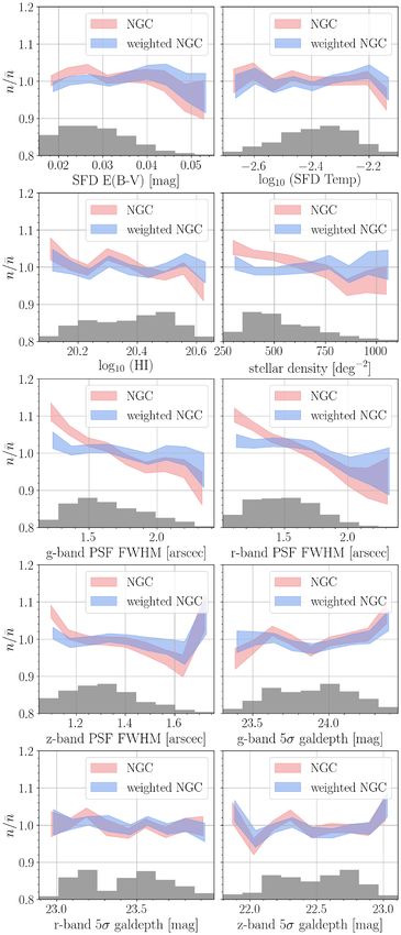
3258         A. Raichoor et al.
Table 2. Reliable redshift statistics for various criteria. We use the last line criterion. Estimate from our catastrophic rates is computed from repeat observations;
see Table 3 for our visual inspection results.

Redshift                                   Criterion                               Reliable           Reliable                 Catastrophic             Catastrophic
fitter                                                                              zspec         0.6 < zspec < 1.1               zspec               0.6 < zspec < 1.1

idlspec1d            Equation (1) of Raichoor et al. (2017)                        83.1%                74.0%                      0.5%                     0.5%
redrock              Equation (3a)                                                 93.0%                82.0%                      0.7%                     0.6%
redrock              Equation (3a) and equation (3b)                               91.8%                81.3%                      0.6%                     0.6%
redrock              Equation (3a), equation (3b), and equation (3c)               90.6%                80.7%                      0.3%                     0.3%

Table 3. Redshift measurement assessment from visual inspection of three              Table 4. Statistic for the ELG sample. The reported N are computed after
plates for ∼1900 ELGs, with 0.6 < zspec < 1.1 and passing equations (3a),             applying the LSS veto masks. A target is either observed or unobserved

                                                                                                                                                                             Downloaded from https://academic.oup.com/mnras/article/500/3/3254/5942664 by guest on 22 February 2021
(3b), and (3c). The visual inspection confidence flag meaning is: 3: definitely       because of close pairs or lack of fibre: Nobs + Ncp + Nmiss = Ntarg . Similarly,
correct, 2: features are visible and the redshift is likely to be correct, 1:         an observed target is classified as a star, as a galaxy, or a redshift failure (i.e.
information in the spectrum, but the redshift is a guess, and 0: no information,      does not pass equations 3): Nstar + Ngal + Nzfail = Nobs . Nused is the number
useless spectrum. For instance, 24.0 per cent of the inspected spectra have           of galaxies with 0.6 < zspec < 1.1. The geometric area is the tiling area, i.e.
confidence = 2, and 99.3 per cent of those have |v| < 300 km s−1 .                   covered by the plates. The unvetoed area is the area after applying the LSS
                                                                                      veto masks. The effective area is the unvetoed area after accounting for the
Conf. Flag       Percentage      |v| < 300 km s−1       |v| < 1000 km s−1           tiling completeness.

3                  71.5%                99.9%                    99.9%                                                    NGC                 SGC               Total
2                  24.0%                99.3%                    99.6%
1                   2.9%                94.5%                    96.3%                Ntarg                              113 500            116 194            229 694
0                   1.6%                 6.5%                     6.5%                Nobs                               106 677            110 314            216 991
All                100%                 98.1%                    98.2%                Ncp                                  5805              4797               10 602
                                                                                      Nmiss                                1018              1083               2 101
                                                                                      Ngal                                94 814            100 271            195 085
confidence flags: 3: definitely correct, 2: features are visible and the              Nstar                                859                845                1704
                                                                                      Nzfail                              11 004             9198               20 202
redshift is likely to be correct, 1: information in the spectrum, but the
                                                                                      Nused                               83 769            89 967             173 736
redshift is a guess, and 0: no information, useless spectrum. Visual                  Geometric area (deg2 )              554.1              616.1             1170.2
inspection results are reported in Table 3. The redrock redshift is                   Unvetoed area (deg2 )               372.8              360.9              733.8
almost in perfect agreement (99.8 per cent with |v| < 300 km.s−1 )                   Effective area (deg2 )              369.5              357.5              727.0
with the inspector redshift for confidence = 3 and confidence = 2                     Effective volume (Gpc3 )             0.30              0.30                0.60
(95.5 per cent of the sample). For confidence = 1 (2.9 per cent of the
sample), both redshift estimations mostly agree (∼95 per cent). For
confidence = 0 (1.6 per cent of the sample), we can conservatively                    a mean difference of v = 16 ± 39 km s−1 (−2 ± 47 km s−1 ) and
assume that the pipeline is wrong in most cases. Overall, based on                    only 1/146 (2/216) objects have v > 1000 km s−1 .
these visual inspections, we estimate that the pipeline provides a                       We thus conclude that the redrock redshift measurements pass-
redshift precision better than 300 km s−1 for 98.1 per cent of our                    ing our equations (3) are precise (precision better than 300 km s−1 for
sample and a catastrophic redshift for ∼1.8 per cent of our sample.                   ∼99 per cent of our sample) and accurate (expected catastrophic rate
   We present a second, independent estimate of catastrophic rate                     of ∼1 per cent), thus fulfilling the eBOSS/ELG requirements set at
with repeat observations, which provides us with ∼17 000 pairs of                     the beginning of the program.
observations of a given target. We restrict to the ∼13 000 repeats
where both redshift estimations pass our reliability criterion and
                                                                                      3 L A R G E - S C A L E S T RU C T U R E C ATA L O G U E S
consider a pair is catastrophic if the two redshift measurements differ
                                                                                      C R E AT I O N
by more than 1000 km s−1 . Following this approach, we find that
0.3 per cent of the sample have a catastrophic redshift measurement.                  We detail in this section the building of the LSS catalogues. These
Additionally, we can assess with repeats that 99.5, 95, and 50 per cent               LSS catalogues are used in this paper to measure the spherically
of our redshift estimates have a precision better than 300 km s−1 ,                   averaged BAO in configuration space. They are also used in de
100 km s−1 , and 20 km s−1 , respectively.                                            Mattia et al. (2020) and Tamone et al. (2020) for the measurement
   Lastly, we assess our redshift measurements with comparing with                    of the growth rate of structures and BAO in Fourier space and in
two external datasets overlapping our eBOSS/ELG footprint: DEEP2                      configuration space, respectively. They are publicly available.12
(Newman et al. 2013), which observations were done with the                              Table 4 summarizes the overall properties of these LSS catalogues.
DEIMOS spectrograph (resolution R ∼ 5900) on the Keck II 10-m                         The steps to build the LSS catalogues are: (1) define starting data
telescope, and WiggleZ (Drinkwater et al. 2010), which observations                   and random samples; (2) define and apply the angular veto masks
were done with the AAOmega spectrograph (resolution R ∼ 1300)                         to the data and the randoms; (3) define weights to correct for non-
on the AAT 3.9-m telescope. When restricting on our eBOSS/ELG                         cosmological fluctuations (redshift failures: w noz , close pairs: wcp ,
sample with a reliable redshift within 0.6 and 1.1, we find 146                       systematics due to photometry: w sys ), and optimize the contribution
matches with DEEP2 objects having a reliable redshift (Q = 4, 5) and
216 matches with WiggleZ objects having a reliable redshift (Q =
4, 5). Our eBOSS/ELG measurements are in good agreement with                          12 Alink to web page will be provided after DR16 papers are accepted for
the DEEP2 and WiggleZ ones: for DEEP2 (WiggleZ), we measure                           publication.

MNRAS 500, 3254–3274 (2021)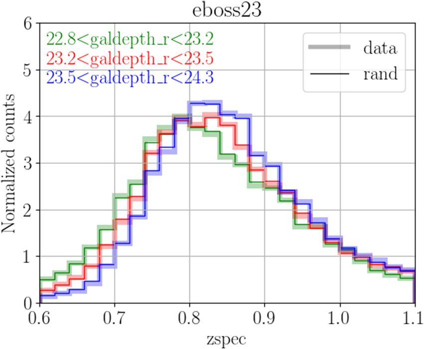
SDSS/eBOSS DR16 ELG LSS and isotropic BAO                                3259
Table 5. Angular veto mask properties. Bits 1, 2, 3, 4, and 5 have been applied      This affects the eboss23 chunk but also – to a lesser extent –
before the target selection (the few removed targets are due to slightly different   the eboss21 and eboss22 chunks; the eboss25 chunk is not
implementation). Apart from the eboss22 two low-quality plates removal,              affected by this mask. This mask can be exactly recovered with using
all veto masks are bit-coded (in the mskbit column in the catalogues).               the legacypipe depth images.
                                                                                        (iii) decam anymask (bit = 3): in the target selection, we re-
Bit                  Mask                    Removed area      Removed targets
                                                                                     quired decam anymask[grz] = 0, where decam anymask is a
                                                (deg2 )
                                                                                     legacypipe quantity, flagging objects where one of the underlying
1     Not g+r+z                                   67.2                  27           DECam images is defective at the pixel position corresponding to
2     xybug                                       49.7                   0           the centre of the object; this flag is often turned on for pixels close to
3     Recovered decam anymask                    210.1                 142           individual imaging CCD edges along the R.A.. In the DECaLS/DR3
4     tycho2inblob                                 4.7                   0           version, the decam anymask information is stored only where
5     Bright objects                              57.6                   7           objects are detected, making it extremely difficult to propagate that
6     Gaia stars                                  54.0              17 456
                                                                                     information to the random sample; however, since the DECaLS/DR7
7     Mira star                                   12.5               3555

                                                                                                                                                                  Downloaded from https://academic.oup.com/mnras/article/500/3/3254/5942664 by guest on 22 February 2021
8     Imprecise mskbit 3                           0.1                  15
                                                                                     version, this information is stored at the pixel level for each brick,
9     centerpost                                   0.6                 166           making it recoverable at any location. We thus re-run the part of the
10    TDSS FES targets                             1.3                 308           DECaLS/DR7 pipeline on the exact DECam imaging data set used
11    DECam bad phot. calib.                      72.7              16 325           for the ELG target selection (smaller than the DECaLS/DR7 one)
–     eboss22 low-quality plates                  13.9               3123            to produce that output, having in this way the decam anymask
–     Total                                      436.5              41 124
                                                                                     information at the pixel level.
                                                                                        (iv) tycho2inblob (bit = 4): in the target selection, we
                                                                                     required tycho2inblob = False, where tycho2inblob is a
of galaxies based on their number density at different redshifts and                 legacypipe column flagging objects whose light profile overlaps
apply inverse-variance weights w FKP ; and (4) assign redshifts to the               one of the Tycho2 stars (Høg et al. 2000). The legacypipe pipeline
randoms.                                                                             stores for each brick that information.
                                                                                        (v) bright objects and Tycho2 stars (bit = 5): we used geometrical
                                                                                     masks to veto the surrounding area of SDSS bright objects13 ; we
3.1 Data selection, random catalogues                                                also define a circular mask for each 0 mag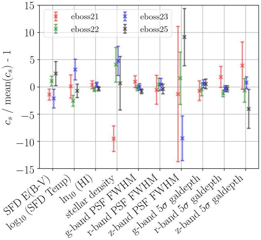
3260          A. Raichoor et al.
for this issue as follows. We use the Healpix16 scheme (Górski et al.
2005) to divide the sky into equal-area small pixels of ∼11 arcmin2
(corresponding to nside = 1024). We reject 37 pixels where the
percentage of objects with an improper recovered decam anymask
is greater than 10 per cent.
    (ix) centerpost (bit = 9): each plate has a hole in its centre to
fix it with the centrepost; as a consequence, no fibre can be placed
within 92 arcsec of the plate centre. Contrary to other BOSS/eBOSS
targets, the higher ELG density making the tiling denser, this does
not result in a ‘simple’ veto mask, as the position of plate centre
can be covered by another adjacent plate (see Fig. 1). However, for
simplicity, we simply mask these centerpost regions.
    (x) TDSS FES targets (bit = 10): on each ELG plate, ∼50 fibres

                                                                                                                                                          Downloaded from https://academic.oup.com/mnras/article/500/3/3254/5942664 by guest on 22 February 2021
are assigned to the Time Domain Spectroscopic Survey (TDSS,
Morganson et al. 2015; Ruan et al. 2016). A subsample of the TDSS
targets, the FES class targets (∼1 deg−2 ), has been tiled with the
same priority as the ELG targets. To account for that, we create          Figure 2. Illustration of the DECaLS-related, bright objects and stars masks
around each TDSS FES target a circular veto mask with a radius of         for a given DECaLS brick (0.25◦ × 0.25◦ , 3600 × 3600 pixels, with
62 arcsec, corresponding to the size of one fibre.                        0.262 arcsec/pixel). The xybug mask is the symmetric along the brick diagonal
    (xi) DECam bad photometric calibration (bit = 11): at the time of     of the not g+r+z mask. The decam anymask mask mostly follows the CCD
DECaLS/DR3, the DECaLS pipeline was including all public grz-             edges along R.A. (horizontal in the figure).
band DECam imaging over the DECaLS footprint, hence imaging
from various different programs. The latest DECaLS/DR8 release17          many zspec measurements rely. As a consequence, redshift failures
mostly restricts to DES and DECaLS observations and has a                 are significant (∼10 per cent of the observations) and present strong
significantly improved photometric calibration procedure. We take         dependencies on observing conditions, which need to be carefully
advantage of that data set to verify the photometric calibration of       modelled and corrected for in the LSS analysis (see, for instance,
our DECaLS/DR3 and DR5 imaging used for target selection. We              Blake et al. 2010; Bautista et al. 2018; Addison et al. 2019).
identify in this way some observing programs with improper photo-            We define the SSR as:
metric calibration (of the order of tens of mmag): such systematic                     Ngal
                                                                          SSR =                 ,                                            (4)
offset in the photometry implies a different target selection, as it              Ngal + Nzfail
is equivalent to move the boundaries of the photometric cuts. We          where Ngal is the number of spectra with a valid fibre, a reliable zspec
remove the regions covered by the DECam CCDs belonging to those           estimate, and not being a star, and Nzfail is the number of spectra
identified observing programs. This mask is displayed in dark grey        with a valid fibre but no reliable zspec estimate and not a star. We
in Fig. 1.                                                                beforehand apply all angular veto masks described in Section 3.2.
    (xii) eboss22 low-quality plates: lastly, we also remove the             To correct redshift failures, we derive weights from a fit of the
regions covered by two eboss22 spectroscopic plates (PLATE-               SSR as a function of two quantities, which correlate with the angular
MJD = 9430-58112 and 9395-58113), which have significantly                position of the fibres on the sky, namely the plate-average SN (pSN19 )
lower-than-average quality. Those plates bias the SSR = f(pSN)            and the (XFOCAL, YFOCAL) position in the focal plane:
fit in equation (6) (see next section). This mask is displayed in black
in Fig. 1.                                                                                         1
                                                                          wnoz =                               ,                                   (5)
                                                                                       fnoz,pSN · fnoz,XYFOCAL
   Fig. 2 illustrates the DECaLS-related, bright objects and stars
masks for a given DECaLS brick.                                              We perform the fit for each half-spectrograph (Spectro 1a: 1 ≤
   We provide in the associated data release the required information     FIBERID ≤ 250, Spectro 1b: 251 ≤ FIBERID ≤ 500, Spectro 2a:
to reproduce the angular masking when considering any (R.A., Dec.)        501 ≤ FIBERID ≤ 750, Spectro 2b: 751 ≤ FIBERID ≤ 1000) of
position: bits 1–7 can compute with the brickmask18 script, bits          each chunk (eboss21,eboss22, eboss23, eboss25). The
8–11 and the two eboss22 low-quality plates can be reproduced             rationale behind this approach stems from the specificity of each
with customed PYTHON lines.                                               chunk and the different response of each half-spectrograph. Indeed,
                                                                          eboss21 has longer spectroscopic exposure time on average and
                                                                          a particular geometry (hence having a non-standard position of the
3.3 Spectroscopic redshift failures                                       fibres in the focal plane), eboss21 and eboss22 have DES, deeper
                                                                          imaging, while eboss23 imaging is shallower and eboss25
The principle of using ELGs for LSS clustering relies on the fact that
                                                                          imaging comes from a different DECaLS release. It is known that
it is possible to measure the zspec thanks to emission lines, with no
                                                                          the second spectrograph (501 ≤ FIBERID ≤ 1000) has a better
requirement of high SN detection of the continuum, making them
                                                                          throughput (Smee et al. 2013): we do observe differences due to this
an interesting tracer. However, for low SN spectra (see Table 1),
                                                                          for our ELG sample, and we also observe that half-spectrographs
the BOSS spectrograph resolution of ∼2000 does not allow the
                                                                          have different responses; for instance, the mean SN per spectra
[O II] doublet to be resolved (Comparat et al. 2013), on which
                                                                          is 0.91, 0.87, 0.94, 0.88 for Spectro 1a, Spectro 1b, Spectro 2a,
                                                                          Spectro 2b, respectively. We currently do not find an explanation
                                                                          for that half-spectrograph difference in the mean SN. For simplicity,
16 http://healpix.jpl.nasa.gov
17 http://legacysurvey.org/dr8
18 https://github.com/cheng-zhao/brickmask/releases/tag/v1.0              19 i.e.   the average SN MEDIAN ALL for the ELG spectra.

MNRAS 500, 3254–3274 (2021)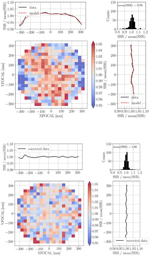
SDSS/eBOSS DR16 ELG LSS and isotropic BAO                               3261

                                                                                                                                                               Downloaded from https://academic.oup.com/mnras/article/500/3/3254/5942664 by guest on 22 February 2021
Figure 3. Fraction of reliable zspec (SSR) per plate, as a function of the plate
SN: each dot represents a PLATE-MJD reduction. For the NGC/SGC, the
SSR before weighting by 1/fnoz,pSN is displayed in green/magenta dots and
the SSR after weighting by 1/fnoz,pSN is displayed in blue/red triangles. The
model is fitted to each half-spectrograph for each chunk.

we display in Figs 3–5 the fitted results for all fibres from each
Galactic cap.
   The first quantity is the overall SN of the plate, pSN. As observa-
tions are performed at a rather low SN, the fraction of redshift failures
increases quickly for lower-than-average observing conditions. In
Fig. 3, we display the plate SSR, i.e. the fraction of reliable zspec per
plate, as a function of the plate SN. We model the SSR dependence
on the plate SN with the following function:
fnoz,pSN (x) = c0 − c1 × |x − c2 |c3 ,                                      (6)
where x is the pSN and the four coefficients c0 , c1 , c2 , and c3 are
fitted through a χ 2 minimization. For each fit, the number of fitted
points is the number of plates per chunk, reported in column (3) of
Table 1. Fig. 3 illustrates how the data populate the pSN, SSR space,
                                                                                   Figure 4. Fraction of reliable zspec (SSR) as a function of XFOCAL and
before (dots) and after (triangles) the weighting by 1/fnoz,pSN . Once
                                                                                   YFOCAL for the NGC, before (top panels) and after (bottom panels)
weighted, the SSR is independent of the plate SN.                                  weighting by 1/fnoz,XYFOCAL . The top- and right-side panels show the SSR
    The second quantity we use is the (XFOCAL,YFOCAL) po-                          as a function of XFOCAL and YFOCAL; the top-right histograms display
sition. On average, fibres from Spectro 1a are at YFOCAL0, from Spectro 1b at YFOCAL0. We model the SSR dependence on                                 Section 4.2. For each fit on the data, i.e. for each half-spectrograph
(XFOCAL,YFOCAL) with the following function:                                       of each chunk, we compare the rms (weighted by the number of
                                                                                   objects in each bin) of the SSR after correction by the redshift
fnoz,XYFOCAL (x, y) = c0 − c1 × |x − c2 |c3 − c4 × |y − c5 |c6 ,            (7)
                                                                                   failure weights, i.e. the weighted rms of the histogram in the right-
where (x, y) are the centre coordinates of bins in the (XFO-                       hand panel of Fig. 3, which we call σ w,pSN . In the baseline case
CAL,YFOCAL) plane, and the seven coefficients c0 , c1 , c2 , c3 ,                  where redshift failures are injected into the mocks deterministically
c4 , c5 , and c6 are fitted through a χ 2 minimization. For each fit,              following their nearest neighbour in the data, virtually all mocks
the number of fitted points is ∼350, the number of bins in the                     have σ w,pSN larger than the data, as expected since the redshift failure
(XFOCAL,YFOCAL) plane. Fig. 4 illustrates the behaviour for                        implementation departs from the fitted model. Additionally, for each
the NGC (Fig. 5 is similar for the SGC). The top panels show                       mock, we generate an alternative version where the redshift failures
the data before the weighting by /1fnoz, XYFOCAL . Some regions                    are injected in a stochastic way with a probability following the
have either systematically lower-than-average (XFOCAL∼−300,                        model predicted SSR of the nearest neighbour in the data. In this
YFOCAL∼−100; or extreme XFOCAL values) or higher-than-                             case, very few mocks (2/1000) have σ w,pSN larger than the data.
average (XFOCAL∼−50, YFOCAL∼50) SSR. Our fitted model                              Using the same criterion for the fit performed in bins of (XFO-
correctly reproduces that behaviour, as one can see from the red line              CAL,YFOCAL), we find a slightly better agreement, with 20/1000
in the side top panels, or in the bottom panels, which display the SSR             having a larger σ w,XYFOCAL . We therefore conclude that the fitted
after weighting by 1/fnoz,XYFOCAL .                                                model may be too simple to fully describe the complex systematics
    In order to quantify the goodness of the fit for equations (6) and             of the data. However, comparing cosmological fits performed with
(7), we use the set of 1000 EZmocks with systematics described in                  the two sets of mocks mentioned above, de Mattia et al. (2020)

                                                                                                                        MNRAS 500, 3254–3274 (2021)
3262        A. Raichoor et al.
                                                                           a sector being a region defined by a unique set of overlapping plates.
                                                                           The tiling completeness is included in the randoms systematic weight
                                                                           wsys and can be seen in Fig. 1.

                                                                           3.5 Systematics due to photometry
                                                                           Once corrected for systematics related to spectroscopic observations
                                                                           (wnoz and wcp ), our 0.6 < zspec < 1.1 data sample still has (angular)
                                                                           imprints of the photometry used for target selection that need to
                                                                           be corrected for. First, in regions with shallow imaging, higher
                                                                           photometric noise implies that more zspec < 0.6 objects than zspec >
                                                                           0.6 objects enter our selection box in the grz diagram, because of
                                                                           the density gradient in that grz diagram; we thus expect to have less

                                                                                                                                                       Downloaded from https://academic.oup.com/mnras/article/500/3/3254/5942664 by guest on 22 February 2021
                                                                           0.6 < zspec < 1.1 objects in shallow imaging regions. Other regions
                                                                           where we expect to have less 0.6 < zspec < 1.1 objects overall are
                                                                           regions with high Galactic extinction (because objects are dimmer)
                                                                           or regions with high stellar density (because each star is likely to
                                                                           blend with an ELG, which was not selected).
                                                                              We include the following systematic photometric quantities as a
                                                                           source of systematics: the DECaLS imaging depth (galdepth, 5σ
                                                                           detection limit for a galaxy with an exponential profile with a radius of
                                                                           0.45 arcsec) and seeing (psfsize) for the three grz bands, the stellar
                                                                           density (estimated from Gaia/DR2), and the Galactic extinction,
                                                                           using E(B−V), dust temperature (Schlegel et al. 1998), and the HI
                                                                           column density (HI4PI Collaboration 2016; Lenz, Hensley & Doré
                                                                           2017).
                                                                              We here describe the method to compute the wsys weights that
                                                                           correct for the systematics coming from the imaging used for the
                                                                           target selection and from Galactic foregrounds. We first apply the
                                                                           veto masks both to our data and random samples. We split the
                                                                           sky in Healpix pixels with nside = 256 (area ∼ 0.05 deg2 ).
                                                                           For each pixel p, we firstly compute the median value sp for each
                                                                           photometric quantity. Then, we compute ndat,p , the number of data
                                                                           weighted by wnoz · wcp , i.e. the number of 0.6 < zspec < 1.1 ELGs
                                                                           corrected for spectroscopic biases. The number of randoms weighted
                                                                           by COMP BOSS, nran,p , is obtained to derive the effective fractional
               Figure 5. Same as Fig. 4, but for the SGC.                  area of each pixel. For each chunk, we proceed to a multilinear fitting
                                                                                                    2
                                                                           with minimizing the χchunk   defined as:
                                                                                                                               2
have shown (their table 5) that the uncertainty in the modelling                      ndat,p − nran,p · ( +
                                                                                                                   s∈S cs · sp )
of redshift failures has a subdominant impact on the clustering            χchunk =
                                                                             2
                                                                                                                                    ,            (8)
                                                                                                           σp
measurements.                                                                        p∈ P

   The total redshift failure weight w noz applied on the data is the      where P is the list of the Healpix pixels inside the considered
inverse product of fnoz,pSN and fnoz,XYFOCAL . To avoid double counting                                                                   √
                                                                           chunk, S is the list of the photometric templates, σp = nran,p
redshift failures, we weight each object by the median SN correction       is the Poissonian error, and ( , cs ) are the fitted parameters. We
to perform the (XFOCAL,YFOCAL) fit (equation 7).                           present in Fig. 6 the fitted cs per chunk, the error bars being
                                                                           estimated from the 1000 fit results on the EZmocks with systematics
                                                                           (Section 4.2). Overall, the fitted cs agree at the 1–2σ level across
3.4 Fibre collision and tiling completeness
                                                                           the four chunks, except for the stellar density, where the eboss21
When two or more targets are closer than the fibre collision radius        chunk has a significantly lower coefficient; this could be explained
(62 arcsec on the sky), they cannot not be spectroscopically observed      by the fact that the stellar density spans significantly higher values
within a single plate. Those targets are said to ‘collide’ and form what   in eboss21 than in the other three chunks. We can then use the ( ,
we call a ‘collision group’ (see Blanton et al. 2003; Reid et al. 2016,    cs ) fitted parameters to define the weight for each Healpix pixel
for more details). This effect has to be corrected in the analysis, as     p:
it artificially changes the clustering of the sample. We weight each                          1
ELG with a valid fibre by the collision pair weight w cp given by          wsys,p =                          .                                 (9)
                                                                                      +       s∈S   cs · sp
the number of targets over the number of valid fibres within each
collision group. Collided or not valid fibres are declared resolved        Figs 7 and 8 display the dependency of the ELG density for each sys-
when they lie in the same collision group as an ELG valid fibre (see       tematics s before (red) and after (blue) applying the computed w sys ,
also Mohammad et al. 2020).                                                for the NGC and SGC, respectively. We see that our computation
   The tiling completeness COMP BOSS is defined as the ratio of            reduces the density variations where they are the strongest, e.g. for
the number of resolved fibres to the number of targets in each sector,     psfsize or the stellar density in the NGC.

MNRAS 500, 3254–3274 (2021)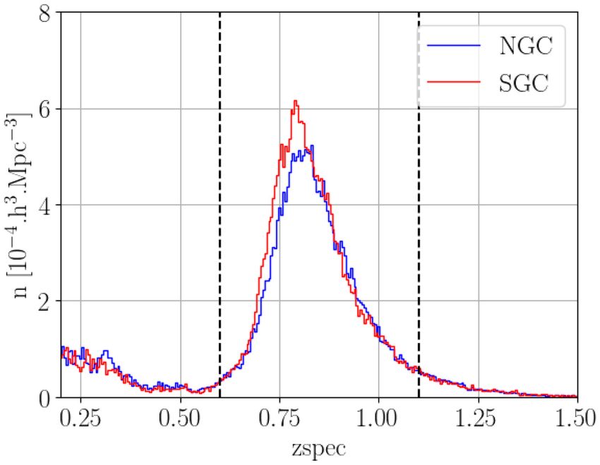
SDSS/eBOSS DR16 ELG LSS and isotropic BAO                                      3263

                                                                                                                                                                     Downloaded from https://academic.oup.com/mnras/article/500/3/3254/5942664 by guest on 22 February 2021
Figure 6. Per-chunk fitted coefficients cs to define the w sys weights (equa-
tion 8). For each systematic photometric quantity, the cs are normalized to the
mean over the four chunks. The error bars are estimated from the EZmocks
with systematics described in Section 4.2.

   We refer the interested reader to Kong et al. (2020), who find
consistent results with a fully independent method. Their approach,
developed in the DESI context and tested on the eBOSS/ELG sample,
consists in injecting fake, realistic sources in the imaging itself,
running the legacypipe photometric pipeline on it, and then
applying the target selection. The strength of that approach is that
it naturally accounts for any possible imaging systematics due to
imaging.

3.6 Weight normalization
The mean of photometric weights wsys of all ELG targets is
normalized to 1 in each chunk. w noz is then scaled such that the
mean of the data completeness weights w sys · wcp · wnoz of ELGs
with a reliable redshift or stars (the latter being assigned w noz = 1) is
equal to the mean of w sys over all resolved fibres. Then targets with
collided or invalid fibres are assigned w cp = 0. Objects that have an
unreliable redshift or stars are assigned w noz = 0.

3.7 Random redshifts and weights
Once cut over the chunk footprint and the angular veto masks, the
randoms have the same angular distribution as data. We then need
to attribute to the randoms redshifts with a similar radial distribution
as the data. We assign redshifts to randoms following the shuffled                Figure 7. Density fluctuations in the NGC for the 0.6 < zspec < 1.1 ELGs
scheme, i.e. picking up zspec values from the data, with a probability            with a reliable zspec , weighted by w noz · w cp , before (red) and after (blue)
proportional to wnoz · wcp · wsys , so that the weighted distributions            applying the w sys weights. The systematics are: E(B–V) and dust temperature,
of data and randoms match.                                                        H I column density, stellar density (from Gaia/DR2), grz-band imaging
                                                                                  seeing, grz-band imaging depth. In each panel, we also display with the filled
   However, we need to account for another effect. The ELG data
                                                                                  grey histogram the distribution of systematics values over the considered
n(z) depends on the depth of the imaging used for target selection                cap.
(markedly for eboss23, but also in the SGC), with n(z) having more
zspec < 0.8 ELGs in shallow imaging regions. Fig. 9 illustrates that
effect for the r-band imaging in eboss23, where the sample is split               imaging depth and apply the shuffled scheme in each subregion.
in three bins of r-band imaging depth. This implies an angular–radial             We define the three subregions with modelling the n(z) as a simple
relation that needs to be accounted for in the randoms.                           function of flux limits. We first define, at any position in the chunk,
   To account for this effect of depth on the target selection process,           fgrz , a combined grz-band imaging depth that correlates best with the
we split each chunk in three subregions of approximately constant                 data zspec . We define fgrz = + cg fg + cr fr + cz fz , a linear combination

                                                                                                                          MNRAS 500, 3254–3274 (2021)
3264 A. Raichoor et al.
Downloaded from https://academic.oup.com/mnras/article/500/3/3254/5942664 by guest on 22 February 2021
Figure 9. Illustration of the dependency of redshift distribution on imaging
depth for the eboss23 chunk, where the dependency is strong. Our randoms
(thin lines) faithfully reproduce the trend of the data (thick lines).
approximately constant depth imaging20 ; the data are binned with
the same three subregions. For a random with a fgrz value, we pick
a redshift from the data zspec from the corresponding fgrz bin, with a
probability proportional to w noz · wcp · wsys . That approach allows
us to reproduce this dependency in the randoms redshifts, as can be
seen in Fig. 9, where the randoms weighted n(z) closely follows that
of the data when splitting by r-band imaging depth. We note that no
significant n(z) dependence is found with the other systematics (listed
in Section 3.5); only a very mild dependence with psfsize g and
psfsize r for eboss23 is seen in the data, but a similar trend
is seen in the randoms, meaning that it is mainly driven by the
dependence with the depth.
For randoms, weights are defined as follows: wsys is the tiling
completeness COMP BOSS, and w noz = wcp = 1. Then, random
weights are normalized to ensure that the sum of weighted data over
the sum of weighted randoms is the same in each chunk z.
Using the shuffled scheme introduces a radial integral constraint
(de Mattia & Ruhlmann-Kleider 2019), which is particularly impor-
tant for this sample, as the random n(z) is tuned to the data n(z) in
small chunks. We correct for that effect with using the formalism
introduced in de Mattia & Ruhlmann-Kleider (2019). Zhao et al.
(2020a) and Tamone et al. (2020) study the impact of that correction
for the different multipoles, for the mocks and the data, respectively.
The monopole is marginally changed, whereas the quadrupole and
the hexadecapole are significantly changed.
Lastly, we remove 163 randoms belonging to tiny sectors where
there are no data with a reliable zspec , which is equivalent to restricting
Figure 8. Same as Fig. 7, but for the SGC. to sectors with COMP BOSS≥0.5 and SSR≥0.
of fg , fr , fz , the 5σ flux detection limits of the imaging at the position 3.8 FKP and redshift distribution
of an ELG in the g-, r-, z-bands. The ( , cg , cr , cz ) coefficients are
As in previous BOSS/eBOSS analyses (e.g. Anderson et al. 2014;
the fitted with minimizing:
Alam et al. 2017; Ata et al. 2018), we define inverse-variance wFKP
Ng weights to be applied to data and randoms. We define w FKP = 1/(1 +
2
2
χgrz = zspec,i − + cg fgi + cr fri + cz fzi n(z) · P0 ) (Feldman, Kaiser & Peacock 1994), where P0 = 4000
i=1 (Mpc/h)3 is the amplitude of the power spectrum at k ∼ 0.1 h Mpc−1 ,
× wnoz
i
· wcp
i
· wsys
i
, (10) a scale at which the FKP weights minimize the variance of the
where the sum is over the Ng ELGs of the chunk. We then bin the
randoms in three bins of fgrz , hence defining the three subregions of 20 Those regions are identified by the chunk z quantity in the catalogues.
MNRAS 500, 3254–3274 (2021)SDSS/eBOSS DR16 ELG LSS and isotropic BAO 3265
Downloaded from https://academic.oup.com/mnras/article/500/3/3254/5942664 by guest on 22 February 2021
Figure 10. Number density of ELGs in the eBOSS survey. The vertical
dashed lines indicate the redshift range used in our clustering measurement.
Table 6. Different cosmologies and redshift used in this paper. h is defined
such that H0 = 100 × h km s−1 Mpc−1 . All cosmologies are flat CDM,
hence = 1 − m . The BAO fits in Section 5 are performed with the
‘DR16 Fiducial’ cosmology.
DR16 fiducial OuterRim EZmocks
h 0.676 0.71 0.6777
m 0.31 0.26479 0.307115
2
bh 0.022 0.02258 0.02214
σ8 0.8 0.8 0.8225
ns 0.97 0.963 0.9611
mν (eV) 0.06 0 0
Redshift zeff = 0.845 zsnap = 0.865 zeff = 0.845
measurement and thus optimize the BAO measurement (Font-Ribera
et al. 2014). Since n(z) varies with the local clustering, the w FKP Figure 11. Effect of the weights on the clustering for the NGC (top panel)
weights tend to upweight (resp. down-weight) underdensities (resp. and the SGC (bottom panel). The vertical lines show the BAO fitting range
overdensities). We did verify that the induced systematic bias is small in this paper.
enough for our analysis.
The redshift distribution of our ELG sample, split by NGC and
SGC, is displayed in Fig. 10. The effective redshift of our sample 4 M O C K C ATA L O G U E S
is zeff = 0.845; as in other eBOSS analyses, zeff is defined as the
In order to validate and perform our BAO fitting method, we rely on
weighted
mean spectroscopic redshift of galaxy pairs (zi , zj ): zeff =
wtot,i wtot,j (zi +zj )/2 two sets of mock catalogues. The cosmology of each set of mock is
i,j
, where wtot = wsys · wcp · wnoz · wFKP and the reported in Table 6. We refer the reader to de Mattia et al. (2020) for
i,j wtot,i wtot,j
sum are performed over all galaxy pairs between 25 h−1 Mpc and more details on those both sets of mocks.
120 h−1 Mpc.
We use the fiducial eBOSS DR16 cosmology (reported in Table 6)
to derive the comoving number density. 4.1 Accurate N-body Sky-cut OuterRim mocks
The first set of mock catalogues used in the subsequent BAO analysis
is the Sky-cut OuterRim mocks, described in de Mattia et al. (2020).
3.9 Effects of weights on the monopole
The starting product is the OuterRim simulation (Heitmann et al.
We display in Fig. 11 how the weights computed in the previous 2019), which is one of the largest high-resolution N-body simulations
sections change the clustering of the ELG sample. As expected (see to date, as it contains 10 2403 particles with a mass of 1.85 · 109
e.g. Ross et al. 2017; Ata et al. 2018), the wsys weights have by far h−1 M over a volume of (3000 h−1 Mpc)3 . Avila et al. (2020)
the strongest impact on the clustering. We notice that the w cp weights have extracted from the OuterRim simulation the snapshot at zsnap =
have an impact at all scales in the SGC and decreasing the clustering: 0.865 and have produced accurate mocks, which faithfully reproduce
a possible interpretation is the ELG SGC chunk geometry, noticeably the DR16 ELG data sample small-scale clustering, using the Halo
eboss21 with its small area. Close pairs should have been missed Occupation Distribution modelling motivated by Gonzalez-Perez
preferentially around the edges and there are more edges because of et al. (2018). From those Avila et al. (2020) mocks, the Sky-cut
the small footprint. Lastly, the w noz weights have a marginal impact OuterRim mocks are generated by cutting the eBOSS/ELG footprint,
on the clustering. applying the veto masks, and reproducing the data n(z) distribution
MNRAS 500, 3254–3274 (2021)3266 A. Raichoor et al.
and accounting for the n(z) dependence with the imaging depth. an orientation of μ.21 We then compute the monopole correlation
Precisely, six nearly independent Sky-cut mocks are extracted from function ξ 0 (s), i.e. the first Legendre multipole with:
the OuterRim box; then, from each of those six mocks, we can extract
four disjoint ELG-like samples and use three line of sight for each 2l + 1 1
ξl (s) = Ll (μ)ξ (s, μ)dμ for l = 0, (12)
sample. 2 −1
We thus have 72 Sky-cut mocks overall but with only six of them where Ll (μ) is the lth -order (0th here) Legendre polynomial.
being almost fully uncorrelated. However, the correlation between We measure the difference in the BAO location between our
the other Sky-cut mocks is not problematic for our analysis, as we clustering measurement and that expected in our fiducial cosmology,
use the Sky-cut mocks to have a representative, mean signal expected which can mostly come either from a difference in projection or from
from our ELG sample (see Section 5.5). the difference between the BAO position in the true intrinsic primor-
dial power spectrum and that in the model, with the multiplicative
fid
shift depending on the ratio rdrag /rdrag , where rdrag is the comoving
4.2 Approximate EZmocks sound horizon at z = zdrag , the redshift at which the baryon-drag
Downloaded from https://academic.oup.com/mnras/article/500/3/3254/5942664 by guest on 22 February 2021
The second set of mocks consists of the 1000 EZmocks realizations optical depth equals unity (Hu & Sugiyama 1996). If we define
2 1/3
presented in Zhao et al. (2020a). The EZmocks are using the the spherically averaged distance DV (z) = DM (z) · czH (z)−1
Zel’dovich approximation (Zel’Dovich 1970) to generate a density as a combination of the Hubble parameter H(z) and the comoving
field and populate galaxies according to the desired tracer bias. As angular diameter distance DM (z), we can express the offset between
for the Sky-cut OuterRim mocks, those EZmocks are cut according the observed BAO location and our template as:
to the eBOSS/ELG footprint, have the veto masks applied, reproduce fid
DV (z)rdrag
the data n(z) distribution, and account for the dependence with the α= . (13)
imaging depth. DVfid (z)rdrag
Additionally, we build another set of 1000 EZmocks, where we Once we have our measurement of α, it can be converted to
include the observational systematics present in the data. The method, an angular location of the BAO, a dimensionless quantity that is
briefly summarized below, is described in details in de Mattia et al. independent of the cosmology:
(2020) to which we refer the interested reader. Angular systematics
are implemented with trimming the mocks – produced at a density DV (zeff = 0.845) D fid (zeff = 0.845)
=α V fid
. (14)
higher than the ELG one – according to a smoothed map of the data rdrag rdrag
observed density, and with adding contaminants (stars or objects
For our fiducial cosmology (‘DR16 Fiducial’ in Table 6), rdrag fid
=
outside 0.6 < z < 1.1), so that the data target density is reproduced 22
on average. Spectroscopic systematics are then implemented with 147.77 Mpc (obtained from CAMB; Lewis, Challinor & Lasenby
introducing realistic fibre collisions (following the plate geometry 2000; Howlett et al. 2012) and DVfid (zeff = 0.845) = 2746.8 Mpc.
and target priority) and redshift failures (using the nearest neighbour We generate a template BAO feature using the linear power
in the data). For each mock, we then compute the weighting scheme spectrum, Plin (k), obtained from CAMB and a ‘no-wiggle’ Pnw (k)
as we do for the data. We remark that, since weights are recomputed obtained from the Eisenstein & Hu (1998) fitting formulae,23 both
on each mock, the noise in the weight calculation due to shot using our fiducial cosmology (except where otherwise noted).
noise and cosmic variance is automatically propagated to the final Given Plin (k) and Pnw (k), we account for RSD and non-linear BAO
cosmological parameters. damping via
Those EZmocks with observational systematics are the ones used
(Plin − Pnw )e−k
2σ 2
P (k, μ) = C 2 (k, μ, s)
v + Pnw , (15)
in Section 5, in particular, to estimate the covariance matrices. The
set of EZmocks without systematics is used only in Section 5.5, where
when comparing to the OuterRim mocks, which have no systematics
included. σv2 = (1 − μ2 ) 2
⊥ /2 + μ2 2
|| /2, (16)
1 + μ2 β(1 − S(k))
C(k, μ, s) = . (17)
5 THE MODEL AND FITTING METHODOLOGY (1 + k 2 μ2 s2 /2)
S(k) is the smoothing applied in reconstruction: S(k) = e−k r /2
2 2
5.1 The model and r = 15 h−1 Mpc for the reconstruction applied to the eBOSS
We measure spherically averaged BAO measurements using the 2- ELG sample (see Section 5.3); S(k) = 0 for pre-reconstruction.
point correlation function. Our methodology closely follows that This matches the implementation of Ross et al. (2017), which was
described in Anderson et al. (2014), Ross et al. (2017), Ata motivated by Seo et al. (2016). For our fiducial analysis, we fix
et al. (2018), and references therein, to which we refer for more β = 0.593 and s = 3 h−1 Mpc. Given this is a spherically averaged
details. analysis that does not consider how the signal changes with respect
We first compute ξ (s, μ), the redshift-space 2D correlation
function as a function of s, the separation vector in redshift space, and 21 The
μ the cosine of the angle between s and the line-of-sight direction. pair-counting is done using the ‘DR16 Fiducial‘, ‘OuterRim’, and
‘DR16 Fiducial’ cosmology for the data, the OuterRim mocks, and the
We use the Landy & Szalay (1993) estimator:
EZmocks, respectively.
DD(s, μ) − 2DR(s, μ) + RR(s, μ) 22 https://camb.info/
ξ (s, μ) = , (11) 23 In order to best match the broad-band shape of the linear power spectrum,
RR(s, μ)
we use ns = 0.963, to be compared to 0.97 when generating the full linear
where DD, DR, and RR are the normalized number of data–data, power spectrum from CAMB. This linear power spectrum is same as used for
data–random, random–random pairs with a separation of s and BOSS and eBOSS galaxy analyses since DR11.
MNRAS 500, 3254–3274 (2021)You can also read