THE ECONOMIC IMPACT OF WEATHER AND CLIMATE1
←
→
Page content transcription
If your browser does not render page correctly, please read the page content below

THE ECONOMIC IMPACT OF WEATHER AND CLIMATE1

                                                                                          Richard S.J. Tola,b,c,d,e,f

                                           a
                                               Department of Economics, Jubilee Building, University of Sussex, Falmer, BN1 9SL, United Kingdom;
                                                                                       r.tol@sussex.ac.uk
                                                      b
                                                          Institute for Environmental Studies, Vrije Universiteit, Amsterdam, The Netherlands
                                                          c
                                                              Department of Spatial Economics, Vrije Universiteit, Amsterdam, The Netherlands
arXiv:2102.13110v3 [econ.GN] 5 May 2021

                                                                            d
                                                                                Tinbergen Institute, Amsterdam, The Netherlands
                                                                                         e
                                                                                             CESifo, Munich, Germany
                                                          f
                                                              Payne Institute for Earth Resources, Colorado School of Mines, Golden, CO, USA

                                          Abstract

                                          I propose a new conceptual framework to disentangle the impacts of weather and climate on
                                          economic activity and growth: A stochastic frontier model with climate in the production
                                          frontier and weather shocks as a source of inefficiency. I test it on a sample of 160 countries
                                          over the period 1950-2014. Temperature and rainfall determine production possibilities
                                          in both rich and poor countries; positively in cold countries and negatively in hot ones.
                                          Weather anomalies reduce inefficiency in rich countries but increase inefficiency in poor and
                                          hot countries; and more so in countries with low weather variability. The climate effect is
                                          larger than the weather effect.
                                          Keywords: climate change; weather shocks; economic growth; stochastic frontier analysis
                                          JEL codes: D24; O44; O47; Q54

                                               1
                                              Marco Letta expertly assisted with data collection and regressions. Max Auffhammer, Peter Dolton,
                                          Jurgen Doornik, Bill Greene, David Hendry, Andrew Martinez, Pierluigi Montalbano and Felix Pretis had
                                          excellent comments on earlier versions of this work. I also thank seminar participants at the EMCC-
                                          III conference, University of Sussex, UNU-MERIT University, the 2019 IAERE conference, Cambridge
                                          University, London School of Economics, Sapienza University of Rome, Shanghai Lixin University, Edinburgh
                                          University, University of Southern Denmark, Federal Reserve Bank of San Francisco, and CESifo.
                                          Preprint submitted to Elsevier                                                                   May 7, 2021
1. Introduction
Climate matters to the economy. Not in the way that classical thinkers such as Guan Zhong,
Hippocrates or Ibn Khaldun, or modern thinkers such as Huntington (1915) or Diamond
(1997) argue it does. Environmental determinism is inconsistent with the observations.
There are thriving economies in the desert, in the tropics, and in the polar circle. There is
destitution, too, in all these places. Climate is not destiny, but it does matter.
The prevailing view among economists, with some exceptions (Bloom and Sachs, 1998,
Sachs, 2003, Olsson and Hibbs, 2005, Barrios et al., 2010), is that climate does not matter for
economic development, only institutions do (Easterly and Levine, 2003, Rodrik et al., 2004).
Some argue that climate and geography partly shaped institutions in the past, but have
become irrelevant since (Acemoglu et al., 2001, 2002, Alsan, 2015). Institutional determinism
is just as inconsistent with the observations. The two halves of the Korean Peninsula and
of the island of Hispaniola are powerful reminders of the importance of institutions, but
climate matters for agriculture (Mendelsohn et al., 1994, Schlenker et al., 2005), for energy
demand (Mansur et al., 2008), for tourism (Lise and Tol, 2002), for transport (Koetse and
Rietveld, 2009), for labour productivity (Kjellstrom et al., 2009, Zander et al., 2015), and
for health (Sachs and Malaney, 2002)—and thus for the economy as a whole.
Climate matters, but it has been an empirical challenge to demonstrate this using country
data. Climate changes only slowly over time, its signal swamped by confounders, many of
which change more quickly than climate. Climate varies substantially over space, but so do a
great many other things that we know are important for development.2 The insignificance of
climate variables in cross-country studies may be due to a lack of statistical power. Indeed,
a climate association is significant in subnational income data (Nordhaus, 2006, Dell et al.,
2009, Desmet et al., 2018, Henderson et al., 2018, Kalkuhl and Wenz, 2020, Conte et al.,
2020, Alvarez and Rossi-Hansberg, 2021) and, as is shown below, in long panels. Because
of the confounders,3 this association cannot be given a causal interpretation.
Unlike the impact of climate, the impact of weather can be identified—or so people have
argued. Identification rests on the fact that weather is random (Heal and Park, 2016),
at least from the perspective of the economy. The problem with this argument is that
by now many different economic activities have been found to be affected by the weather
(see Auffhammer and Aroonruengsawat, 2011, Barreca et al., 2016, Deschenes and Green-
stone, 2007, Graff Zivin et al., 2020, Leightner, 1999, Li et al., 2018, Pechan and Eisenack,
2014, Ranson, 2014, Zhang et al., 2018, among others), and these activities impact one an-
other.footnoteMérel and Gammans (forthcoming) shows that non-linear panels with weather
but no climate variables are biased.

   2
     Druckenmiller and Hsiang (2018) propose the solve the confounding problem by spatial differencing,
which works if the variable of interest changes at a finer resolution than its confounders, but may work less
well if data are measured on different and irregular grids.
   3
     Andersen et al. (2016) argue that it is UV radiation, rather than climate, that affects development.

                                                     2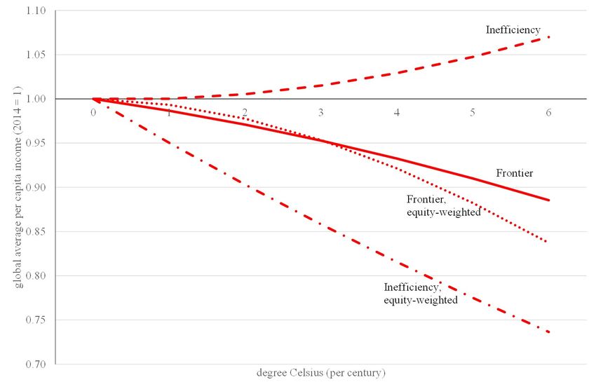
Causality notwithstanding, these studies show that weather matters to the economy. How-
ever, the impacts of weather shocks cannot readily be extrapolated to the impacts of climate
change (Dell et al., 2014, Kolstad and Moore, 2020). Climate is what you expect, weather is
what you get. Weather are draws from an probability distribution. Climate is that distribu-
tion. Climate change shifts the moments of the weather distribution (Auffhammer, 2018b).
Weather is unpredictable for more than a few days ahead. Adaptation to weather shocks
is therefore limited to immediate responses—put up an umbrella when it rains, close the
flood gates when it pours. Adaptation to climate change extends to changes in the capi-
tal stock—buy an umbrella, build flood gates. Furthermore, adaptation to climate change
depends on updates of the expectations for weather (Severen et al., 2018, Lemoine, 2017,
Bogmans et al., 2017). In other words, weather studies estimate the short-run elasticity,
whereas the long-run elasticity is needed to estimate the impact of climate change.
Hsiang (2016) and Deryugina and Hsiang (2017) argue that the marginal effect of a weather
shock equals the marginal climate effect. Climate change is not marginal but its total impact
is an integral of marginals. Their assumptions are quite restrictive, however. Economic
agents need to be (1) rational and their adaptation investments (2) optimized. Adaptation
needs to be (3) private and adaptation options (4) continuous. The economy needs to be in
a (5) spatial equilibrium and (6) markets complete. Adaptation investments are often long-
lived, so both spot and future markets should be complete. Spatial zoning and transport
hubs distort the spatial equilibrium. Adaptation is often lumpy, be it air conditioning or
irrigation. Some adaptation options, such as coastal protection, are public goods. Other
adaptation options, such as protection against infectious disease, have externalities. Agents
are not always rational, and decisions suboptimal. The result by Deryugina and Hsiang is
almost an impossibility theorem.
Weather affects economic activity, and so the measurement of the impact of climate on
economic activity. Weather can be seen as noise, but that noise may well be correlated
with climate, the right-hand-side variable of interest. I therefore propose a new way to
simultaneously model the impact of climate and weather, to show that both matter and
that previous work is misspecified.
The empirical strategy rests on the following assumptions. Climate affects production pos-
sibilities. This is obvious for agriculture: Holstein cows do well in Denmark but jasmine
rice does not; the reverse is true in Thailand. Climate also affects energy and transport,
and thus all other sectors of the economy. Weather affects the realization of the production
potential. Hot weather may slow down workers, frost may damage crops, floods may disrupt
transport and manufacturing. Conceptualized thus, climate affects the production frontier,
and weather the distance from that frontier. The econometric specification is therefore a
stochastic frontier analysis with weather variables in inefficiency and climate variables in the
frontier.4 Climate affects potential output, weather the output gap.

  4
    Kumar and Khanna (2019) estimate the impact of temperature and rainfall on inefficiency in output
growth. I here study inefficiency in output. They omit climate from the frontier.

                                                 3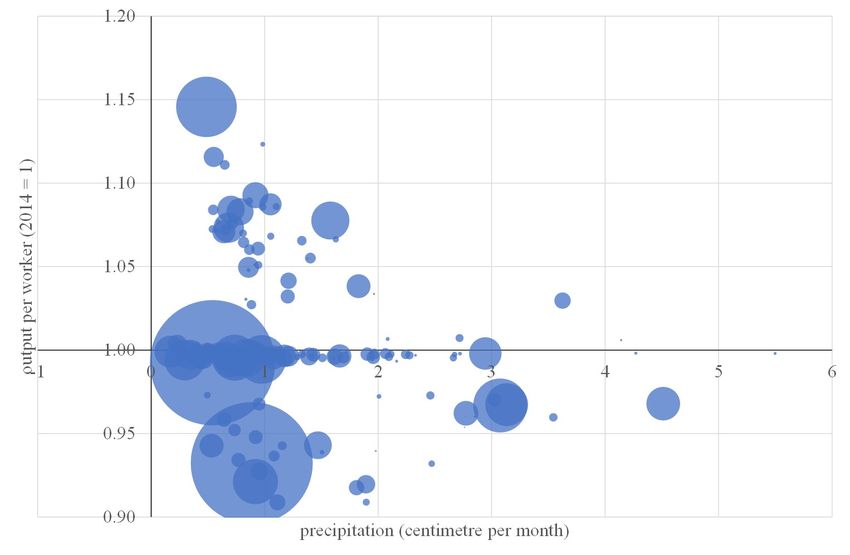
I apply the proposed method to a panel of output per worker, measured at the country
level. Dell et al. (2012), Letta and Tol (2018) and Newell et al. (2018) find that weather
shocks hit the economic growth of poorer countries harder. Burke et al. (2015) instead
find that hotter countries are hit harder, a specification adopted by Pretis et al. (2018),
Henseler and Schumacher (2019) and Kalkuhl and Wenz (2020). Generoso et al. (2020) has
a similar result. Within sample, it is difficult to distinguish between these two specifications
as hotter countries tend to be poorer. However, out of sample, a hotter, richer world would
be more vulnerable to weather shocks according to Burke, but less vulnerable according to
Dell. Kahn et al. (2019) reject heterogeneity. The results below shed new light on these
questions.
Moore and Lobell (2014) regress farm profits on the thirty-year average temperature and
rainfall, and the quadratic deviation from that average, thus accounting for both climate and
weather. Heutel et al. (forthcoming) regress mortality on weather, but interact the weather
effect with climate zones. Auffhammer (2018a) proposes a two-level hierarchical model with
the impact of weather at the bottom and its interaction with climate at the top.5 In the
model below, climate and weather interact too, but in a more intuitive way: Climate affects
potential output, weather the output gap; the impact of climate is deterministic, while the
effect of weather is stochastic.
The cross-validation study of Newell et al. (2018) finds that weather affects the level of
GDP rather than its growth rate, a specification adopted here in line with the intuition
sketched above. Furthermore, I assume that the economy is affected by unusual weather
rather than weather. Frost of -10℃ brought Texas to a standstill in February 2021, but is
a regular occurrence in North Dakota without major consequences. I therefore standard-
ize the weather, expressing temperature and precipitation in standard deviations from the
mean. This introduces an interaction between weather and climate, and an implicit model
of adaptation.
The paper proceeds as follows. Section 2 describes methods and data. Section 3 presents
the baseline results. Section 4 conducts the sensitivity analysis. Section 5 discusses the
implications for climate change. Section 6 concludes.

2. Methods and data
2.1. Methods
I assume a Cobb-Douglas production function:
                                                       β 1−β
                                          Yc,t = Ac,t Kc,t Lc,t                                        (1)

Total factor productivity Ac,t is the Solow residual in country c at time t: It captures
everything that affects output Yc,t that cannot be explained by capital Kc,t or labour Lc,t .

   5
    Bigano et al. (2006) use a similar model for tourist destination choice, with climate at destination at
the bottom and climate at origin at the top.
                                                    4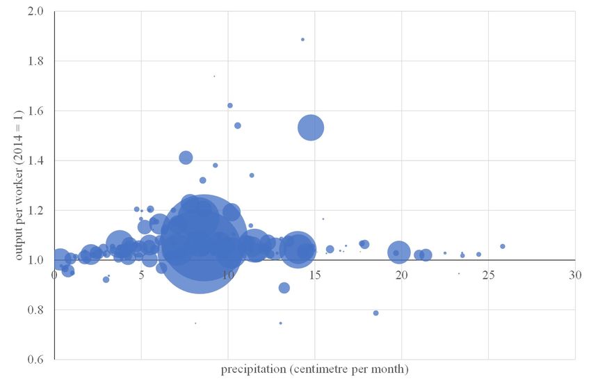
I concentrate Equation (1) by dividing K and L by labour force L, and denote the resulting
variables in lower case.
Taking natural logarithms, the equation to be estimated is:

                                          ln yc,t = α + β ln kc,t                                        (2)

I assume that total factor productivity is a function of moving averages of weather variables
(average temperature, T̄c,t , and precipitation, R̄c,t ). This is loosely based on Nordhaus
(1992). Weather shocks affect the variance of the stochastic component of permanent income.
Hence, Equation (2) becomes:

                    ln yc,t = β1 ln kc,t + f T̄c,t , R̄c,t + µc + t + vc,t − uc,t         (3)

where T̄c,t and R̄c,t are the average temperature c.q. precipitation in country c in the thirty
years preceding year t, µc is a full set of country fixed effects, t is a linear time trend,
vc,t ∼ N (0, σv2 ) and

                                                 Tc,t − T̄c,t            Rc,t − R̄c,t
                 uc,t ∼ E(λc,t ) = E γ0 + γ1 g                  + γ2 g                      (4)
                                                     τc,t                    ρc,t

where τ and ρ are the standard deviations of temperature and rainfall, respectively. Instead
of the unwieldy T − T̄ /τ , I write z(T ); ditto for R. This is standardized temperature and
                                                                            2                     2
precipitation. In the base specification, f T̄c,t , R̄c,t ≡ β2 T̄c,t + β3 T̄c,t + β4 R̄c,t + β5 R̄c,t +
β6 T̄c,t R̄c,t , a second-order Taylor approximation, and g(·) ≡ | · |. I refer to Equation (3) as
the frontier or potential output, and to Equation (4) as inefficiency or the output gap.
Note that in this specification, the impact of weather is stochastic. Unusual weather affects
the mean and standard deviation of the output gap.
I use the True Fixed-Effect (TFE) model (Greene, 2005) to estimate a one-step stochastic
frontier model in a fixed-effect setting with explanatory variables in the inefficiency pa-
rameter. I use the sfmodel package for Stata (Kumbhakar et al., 2015) to estimate the
model.
Equation (3) assumes that both error terms are stationary. This is a tall assumption.6 I
am not aware of any statistical test for stationarity that applies to this particular estimator
and these distributional assumptions.7 I use three remedies. First, I include a time trend in
Equation (3), and try many variants of that trend. Second, I show robustness to different
specifications. Third, I reformulate the model as an error-correction one. The output gap
follows
                  ∆ ln yc,t = ψ1 ∆z (Tc,t ) + ψ2 ∆z (Rc,t ) + ψ3 Vc,t + µc + wc,t           (5)

   6
     Taking first differences of all variables may get rid of unit roots in the frontier but would change the
distributional assumptions in inefficiency.
   7
     Rob Engle (personal communication) suggests that standard stationary tests would roughly apply here.
                                                     5
where potential output is
Vc,t = ln yc,t − µc − µt − ϑ1 ln kc,t − f (T̄c,t , R̄c,t ) (6)
and µt are time dummies which act as a non-parametric time trend.8 This alternative
estimation strategy shows that the findings are robust to the inclusion of non-parametric
time trends. This alternative specification is also better suited to explicitly model the path of
convergence towards the long-term equilibrium in a stochastic setting and provide empirical
evidence for the speed of recovery after weather perturbations. I of course also perform the
usual stationarity tests on the error-correction model.
I test for heterogeneity by interacting the variables of interest with dummies for poor coun-
tries and hot countries. I define a country as “poor” if the World Bank does.9 Alternative,
a country is deemed poor if its GDP per capita was below the 25th percentile of the distri-
bution in the year 1990.10 A “hot” country is defined as a country whose average annual
temperature is above the 75th percentile of the distribution.
2.2. Data
The dataset is an unbalanced panel consisting of 160 countries over the period 1950-2014.11
Data for this study come from two sources. Economic data on output, capital and labour
force are taken from the Penn World Table (PWT), PWT 9.0 (Feenstra et al., 2015). Weather
data are from the University of Delaware’s Terrestrial air temperature and precipitation:
1900-2014 gridded time series, (V 4.01) (Matsuura and Willmott, 2015). These gridded
data have a resolution of 0.5 × 0.5 degrees, corresponding roughly to 55 × 55 kilometers at
the equator. Following previous literature (Dell et al., 2014, Burke et al., 2015, Auffhammer
et al., 2013), we aggregate these grid cells at the country-year level, weighting them by
population density in the year 2000 using population data from Version 4 of the Gridded
Population of the World.12 , with the exception of Singapore.13 We use these weather data to
construct both the climate and weather variables as defined in Section 2.1. Table 1 presents
descriptive statistics for the key variables.14
8
The use of a non-parametric time trend was not possible in the baseline SFA model because the inclusion
of so many time dummies causes convergence issues in an already computationally cumbersome maximum
likelihood estimation.
9
The WB classification of high-income economies is available here.
10
1990 is the first year for which we have complete data on PPP GDP per capita for all countries. I choose
the 25th percentile of the income distribution because, after testing the 25th, 50th and 75th percentiles, the
specification using the 25th percentile resulted the best one according to the Wald Test.
11
Data are not missing randomly (Baltagi and Song, 2006). Warmer countries tend to have shorter records.
This is confirmed by a panel fixed-effect logit regression of having GDP data on the same climate variables
as in the base specification below. The correlation between the residuals of the base specification and the
logit model is -2.2%. Selection bias is therefore minimal.
12
Available here.
13
Singapore has a surface smaller than the size of the weather grids. Given it is one of the few countries
that are both rich and hot and thus increase the statistical power of the analysis, we kept it in the sample
by attributing to it the weather data of the grid cell in which it is situated.
14
See the Appendix for a complete list of countries and regions in the sample.
63. Results
Table 2 shows the results of the base specification outlined in Equations (3) and (4). Six
variants are presented. Column 1 reports homogeneous effects in both the frontier and
the inefficiency. In the frontier, capital per worker has a significant impact on output per
worker. The output elasticity is around 0.63, in line with previous estimates. This estimate
is robust to specification. Long-run temperature (i.e. climate) has a significant impact on
the production frontier, but precipitation does not, as in earlier papers (Dell et al., 2012,
Burke et al., 2015, Letta and Tol, 2018). Short-term weather anomalies, either temperature
or precipitation, are insignificant in determining inefficiency.
Columns 2 and 3 show heterogeneous impacts between rich and poor countries. The hy-
pothesis is that poor countries are disproportionately affected by climate and weather, as
economic activity is concentrated in agriculture and public investment in protective mea-
sures is limited. Column 2 allows heterogeneity only in the production frontier. That is,
I interact climate variables with the poor country dummy defined in Subsection 2.1. The
interaction terms are individually insignificant. Column 3 adds heterogeneity in inefficiency.
Results for the production frontier are almost unchanged. Impacts on inefficiency sharply
differ among rich and poor countries: the latter suffer from large and strongly significant
effect of temperature and rainfall anomalies, whereas the impact is smaller and positive in
rich countries.
Column 4 adds more heterogeneity in inefficiency by interacting weather anomalies with
the ’hot country’ dummy defined in Section 2.1. These interactions are significant, and
strengthen the significance of other parameters in the efficiency. Previous findings had
either poor countries (e.g. Dell et al., 2012, Letta and Tol, 2018) or hot countries (Burke
et al., 2015) particularly vulnerable to weather anomalies. I find both.
Columns 1-4 specify that, in the frontier, hot and cold countries respond differently to
temperature, and dry and wet countries differently to rainfall. Column 5 adds the interaction
between rainfall and temperature to the frontier. This interaction is negative, but less so in
poor countries. The rainfall terms are now significant too: Wetter countries are richer, and
this effect is weaker for poor countries.
Dropping the insignificant interaction terms between temperature and poverty (column 6)
hardly affects the parameter estimates. Column 6 is the preferred specification.
Weather anomalies increase inefficiency in poor countries, as expected. Weather anomalies
decrease inefficiency in rich countries—that is, unexpectedly much or little water, or unusu-
ally hot or cold weather stimulate the economy. This is harder to explain. It may reflect the
restoration effort after floods, and crop insurance and government support after droughts.
The data are GDP rather than NDP, and thus suffer from Bastiat’s broken window. This
effect is not observed in poor countries because restoration after natural disasters is limited
and delayed (Cavallo and Noy, 2011).
I interpret the effect size below, after discussing the robustness of the results.
74. Robustness
I implement three different types of robustness checks: sensitivity to different specifications
in the SFA model; an alternative distributional assumption for the inefficiency parameter;
and an error-correction model to formally test for non-stationarity. For all these sensitiv-
ity tests, with the exception of the error-correction model, I only report estimates of the
preferred specification, column 6 of Table 2.
4.1. Alternative specifications
This first set of robustness checks implements the same baseline model described in Equa-
tions (3) and (4) but adopts a broad set of different specification choices for key variables
and interactions.
4.1.1. Poor v rich
I test whether the core findings are driven by the somewhat arbitrary discrimination between
rich and poor countries. I replace the World Bank classification of countries that are rich15
by the “poorest 25% in 1990”. Results are in column 2 of Table 3. Column 1 repeats the
base specification (column 6) of Table 2.
For the production frontier, results are qualitatively the same as in Table 2. The main
difference is that precipitation loses much of its predictive power, highlighting that different
economies do respond differently to the availability of water resources. As for the inefficiency,
results are again qualitatively similar to the baseline model, but coefficients are closer to
zero and less significant. The log-pseudolikelihood is much lower.
4.1.2. Squared anomalies
Second, I replace absolute weather anomalies in the inefficiency term with squared anomalies.
This places a heavier weight on larger anomalies. See column 3 of Table 3. The results for
the production frontier are largely unaffected, and the qualitative results for the inefficiency
are as above. The log-pseudolikelihood falls.
4.1.3. Linear anomalies
The weather anomalies in Equation (4) are absolute anomalies. Cold and hot weather, wet
and dry spells are assumed to equally increase technical inefficiency. Column 4 of Table 3
instead use the anomalies. Estimates for the production frontier are almost unaltered. The
parameters for inefficiency become insignificant. Economies are affected by unusual weather,
rather than by the weather per se. Adaptation matters.
4.1.4. Asymmetric anomalies
I also test for asymmetric anomalies, disentangling negative and positive weather shocks on
inefficiency. This is the preferred specification of Kahn et al. (2019). Results are in column
5 of Table 3. The frontier is not affected. The results are much as above, with anomalous
15
Available here.
8weather being good for rich countries but bad for hot and poor countries. While there is
some evidence for asymmetry between the impact of wet and dry spells, cold and hot spells,
the increase in the log-pseudolikelihood is minimal (less than 6 points) for the six additional
parameters estimated.
4.1.5. Weather in the frontier
I also look at weather effects on productivity, moving weather anomalies from the inefficiency
parameter to the production frontier. Results are in column 6 of Table 3. The frontier does
not change. Coefficients of weather variables are individually insignificant and the log-
pseudolikelihood is sharply lower. This specification, variations of which are often used in
literature, is not the preferred one.
4.1.6. Half-normal distribution
Equation (4) assumes an exponential half-normal distribution for inefficiency. Column 7 of
Table 3 show results for the half-normal distribution.16 The estimates for the frontier are as
above. The inefficiency parameters are much the same, but the interactions with heat lose
significance.
The log-pseudolikelihood falls. One key difference is that the standard deviation of the
inefficiency
√ equals its expected value for the exponential distribution, but its expected value
times 0.5π − 1 for the half-normal distribution. The data are overdispersed for the half-
normal.
4.2. Institutions
4.2.1. Capital as a substitute for climate
I find a significant association between climate and economic performance. In the con-
centrated Cobb-Douglas production function, Equation (1), there are two determinants of
output per worker: climate and capital per worker. In this specification, capital is a de
facto substitute for climate, with a constant elasticity. I test that assumption, answering
the question whether sufficient capital would make a country immune from the influence
of its climate. I therefore interact long-run temperature variables with capital per worker
in the production frontier. See Table 4, Columns 2 and 3; column 1 reproduces the base
model from Table 2. Rainfall is significant and so are its interactions with capital. The in-
teractions have the opposite signs. That is, climate’s influence on output shrinks as capital
deepens. The interaction between temperature, rainfall and capital is insignificant. The log-
pseudolikelihood increases by 7 points. However, interactions work both ways. The output
elasticity of capital now depends on rainfall, varying between 0.73 in the driest countries
and 0.93 in the wettest ones. A 5.5% increase in rainfall, well within the climate change
projections for this century, would lead to increasing returns to scale and explosive economic
growth. I therefore keep the base specification as is.
16
Truncated-normal models with fixed-effects are known to suffer severe convergence issues, and this case
was no exception. It is therefore excluded.
9Column 2 only changes the frontier. In column 3, I replace the interaction with the poverty
dummy by an interaction with capital per worker. Signs change and the log-pseudolikelihood
falls. Poverty is more than a lack of capital, and poverty drives vulnerability to weather
shocks.
4.2.2. Institutions vs climate
In the debate on the long-run determinants of growth and development, some find that
climate plays a fundamental role in shaping long-run development, whereas others argue
that the impact of climate disappears when accounting for institutions, although climate
may have shaped those institutions. I test this in column 4 of Table 4. As a proxy for
institutional quality, I use the Polity2 Score.17 This categorical variable is an aggregate
score which ranges from -10 (hereditary monarchy) to 10 (consolidated democracy). While
this is not the best indicator for institutional quality, it is correlated with other indicators.
Historical depth is the key advantage of Polity2 over other indicators, which are available
only for recent years. I interact it with long-run precipitation in the production frontier.
The results for inefficiency are essentially the same as in the base specification. In the
frontier, the impact of temperature and capital is unchanged. However, the effect of rainfall
is very different. Polity2 and its interactions have an insignificant effect.
4.3. Cointegration
Non-stationarity is a key concern in any long panel of economic data. The residuals of the
stochastic frontier model do not pass a stationarity test. See Table A1. Panel stationarity
tests require that the residuals of every country are stationary. Equation (3) has a common
trend for all countries. The panel is unbalanced, with fewer observations for hotter and
poorer countries in the early years. It should therefore not come as a surprise that the
model fails the test for panel cointegration.
Table A2 shows the results if the model is estimated without a trend, a linear trend (as
above), and a polynomial trend of order two or three; and if a different linear trend is used
for poor and for other countries. Qualitatively, the impact of climate and weather is the
same. The differences between estimates are not significant. Although the residuals of the
alternative models are not stationary (results not shown), the stability of the results suggest
that the regression results are not spurious.
Table A1 supports that suggestion. Output and capital per capita are non-stationary, but
the climate and weather variables are. That means that the residuals of the model are non-
stationary because output and capital do not cointegrate (after inclusion of a trend). The
impact of climate and weather on output per worker is not spurious—climate and weather
do not explain the residual trend in output because there is no trend in the climate and
weather data.
17
The Polity Project Database, annual national data for the period 1800-2017, can be downloaded here.
10The rightmost columns of Table A1 re-estimate the model in first differences. Note that
the difference between two exponential distribution is not an exponential distribution; an
stochastic frontier model in first differences is a different specification. The second-to-
rightmost column estimates the frontier in first-differences and adds lagged variables to
inefficiency. Reassuringly, the output elasticity of capital does not significantly change when
the model is estimated in first differences. The impact of weather and climate either becomes
insignificant or much smaller.
In the rightmost column, I estimate the frontier in first differences, adding the first difference
of the estimated inefficiencies in the base specification (column (6) in Table 2, colum “linear”
in Table A1). Inefficiency enters without explanatory variables. This is a different speci-
fication than the base one—the sum of exponential distributions is not exponential—and
two-stage estimation is inefficient. That said, the signs and significance of the coefficients
are as in the base specification. Estimated values are different from the base specification
for temperature, precipitation and their interaction. The bottom row of Table A1 shows
that differencing does not solve the cointegration problems—economic growth is too variable
over time and space to be captured by a simple model.18 Qualitatively, however, the results
remain—the impact of climate on the frontier is not spurious.
4.4. Error-correction model
As a further empirical test, I estimate the error-correction model (ECM) defined in Equa-
tions (5) and (6). I assume that weather anomalies cause short-term deviations from the
long-run equilibrium, while climate affects the long-run equilibrium growth path of the econ-
omy. The error-correction model is dynamic, unlike the stochastic frontier models above,
tracking the time needed to absorb the perturbation caused by weather anomalies. The
ECM specification allows for country and year fixed-effects, replacing the linear time trend
in the stochastic frontier.
Table 5 presents the results for the long-run co-integrating vector, Table 6 for the short-run
error-correction. In the short-run error-correction estimates, V is the residual of Table 6,
Column 4, since this specification fits the data best.
The output elasticity of capital in the co-integrating vector is much the same as above.
The climate variables and their interactions with the poverty dummy are not individually
significant, with a few occasional exceptions, but the log-pseudolikelihood reveals that they
are jointly significant: 162 points gain for 10 parameters. This is confirmed by Table A4:
Without the climate variables, the Im et al. (2003) test firmly rejects the null-hypothesis
that the residuals are stationary.
The cointegrating vector and the stochastic frontier model have the same signs on the
climate variables and on their interactions with poverty. Qualitatively, the above findings
are confirmed.
18
I re-estimated the model with country fixed-effects in first differences (results not shown); the impact
of climate on the frontier is not materially affected, but the residuals do not become stationary.
11Table A4 shows that the residuals of the short-run equation are stationary. Table 6 shows
the estimates. The cointegrating vector is highly significant. The parameter estimate of
0.06 indicates rather fast convergence to the equilibrium relationship. Precipitation is not
significant but temperature is, in poor countries. This result is qualitatively different from
the stochastic frontier model—but similar to Dell et al. (2012).
Note that the results in Table 6 are for the standardized temperature and precipitation,
rather than their absolute values. This is a further deviation from the stochastic frontier
model. Table A3 shows the results for the absolute anomalies. The results are much the
same, except that temperature now also affects rich countries. The log-pseudolikelihood is
lower, however.
5. Implications
The impact of climate change is highly nonlinear in this model. The effect size is therefore
hard to grasp. Furthermore, there are 160 countries in the database. There are many
scenarios and models of climate change, and many scenarios and models of future economic
growth. Exploring all possible futures is a combinatorial explosion, and would shed little light
on how the model presented here works. So instead, I used stylized scenarios to illustrate
the impact of climate change, according to column 6 in Table 2, on the 2014 population,
economy and climate.
The production frontier, Equation (3), depends on the thirty-year average of the level of
temperature and precipitation. This is projected to change over time. Inefficiency, Equation
(4), depends on the absolute value of the standardized temperature and rainfall. Without
climate change, there are weather shocks to inefficiency and hence economic output. With
climate change, weather shocks are different.
I consider warming between 1℃ and 6℃, and 0.01℃/year and 0.06℃/year. This is the
range shown in the Fifth Assessment Report of the Intergovernmental Panel on Climate
Change (IPCC). I let rainfall increase or decrease by up to 30%, again within the range of
expectations for this century. The impact of these scenarios on the frontier is immediate.
The impact of climate change on inefficiency follows from the deviation of the actual weather
from the expected weather. Without climate change, the expected temperature shock is zero.
With a 3℃ per century warming, the expected temperature shock is 15 × 0.03/τc per year,
where the factor 15 is there because I use the 30-year average and standard deviation for
normalization.
Climate affects production possibilities, and anomalous weather the realisation of those
possibilities. Climate change will affect both. Extrapolating statistical models is always
tricky. Here, the frontier is estimated on a wide range of climates, while inefficiency depends
on time-varying standardization of weather variables. Both help to make extrapolation more
reliable.
12Figure 1 shows the global average impact, separately for changes in temperature and pre-
cipitation. The impact on the frontier is not out of line with previous studies (Tol, 2018): A
5% loss for 3℃ warming. The function is almost linear. The impact on inefficiency is more
non-linear, but smaller and positive because the impact on rich countries dominates.
This is confirmed by the second set of graphs in Figure 1. The above results compute
the global average output. The two remaining graphs compute the global average utility,
expressed in its income equivalent, assuming a rate of risk aversion of one (Fankhauser et al.,
1997). At the frontier, these equity-weighted impact are more linear and larger if warming
exceeds 3℃. This is because poorer countries are hit harder by climate change at the frontier.
This is more pronounced in inefficiency: The sign flips, and the global average impact is
substantially larger than on the frontier.
The right panel of Figure 1 show the impact of changes in precipitation. At the frontier,
the impacts are large. Drying would be a loss, wettening a gain. These impacts are less
pronounced if the national impacts are equity-weighted. This follows from Table 2: Poor,
hot countries have smaller parameters. For inefficiency, change matters rather than the
direction of change; inefficiency is determined by deviations from experience, regardless of
whether that deviation is more or less water than expected. The impacts are more modest.
Equity-weighting again flips the sign: Poor countries are negatively affected, rich countries
positively.
Figure 2 shows the results by country, for a 3℃ warming and a 20% increase in precipitation
over a century. In all figures, the size of the bubble is proportional to the population size in
2014.
The top left figure shows the impact of warming on the frontier, plotted against the average
temperature for 1985-2014. The spread is quite large, ranging from a 90% increase to a 70%
decrease. Colder countries see more positive impacts, hotter countries more negative ones.
The figure separates poor countries—which are essentially on a continuous lines—and rich
ones—which are more dispersed because the impact of wealth is interacted with precipita-
tion. Richer countries face more negative impacts.
The top right figure shows the impact of warming on inefficiency, plotted against the standard
deviation of the temperature for 1985-2014. Effect sizes are smaller than on the frontier,
ranging between a 20% decline and a 15% increase, and fall for countries with greater climate
variability. There are three separate graphs, corresponding with the interactions in Table
2. Rich countries see benefits, poor but cool countries moderate losses, and poor and hot
countries large losses.
The bottom left figure plots the impact of wettening on the frontier against average precipi-
tation in 1985-2014. Heterogeneity is again large, ranging from the 15% loss to a 90% gain.
There is little structure in the graph.
The bottom right figure plots the impact of wettening on inefficiency against the standard
deviation of precipitation in 1985-2014. Effect sizes are smaller than on the frontier, ranging
13between a 10% loss and the 15% gain, and fall with greater climate variability. There are
again three separate graphs. Rich countries see gains, poor and cool countries small losses,
and poor and hot countries large losses.
6. Discussion and conclusion
I use stochastic frontier analysis to jointly model the impacts of weather and climate on
economic activity in most countries over 65 years. I distinguish production potential, affected
by climate, and the realisation of economic output, affected by weather. Weather shocks thus
have a transient effect, climate change a permanent impact. Warming affects production
potential, positively in cold, negatively in hot countries; and more so in rich, wet countries.
Changes in precipitation also affect the frontier. The impacts are heterogeneous without an
obvious pattern. Climate change also affects inefficiency, particularly in countries with little
climate variability, reducing the output gap in rich countries but increasing it in poor and
hot countries. The weather effect is small compared to the climate effect. These results are
qualitatively and quantitatively robust to alternative specifications, controls, and estimators.
Dell et al. (2012) find that poor countries are particularly vulnerable to weather shocks,
Burke et al. (2015) find that hot countries are. In the Burke (Dell) specification, countries
would grow more (less) vulnerable to unusual weather in a hotter and richer future. I find
that both are true, and that the impact of heat is about as strong as the impact of poverty.
Reduced outdoor work and manual labour, decreased relative importance agriculture in
output and work force, and greater diffusion of adaptive capital such as air conditioning
would help poorer countries to dampen the negative effects of weather shocks—but only to
a degree, as the effort needed to alleviate the heat rises with the temperature.
The impact of weather shocks found here cannot directly be compared to previous studies.
Letta and Tol (2018) model economic growth as a function of the change in temperature,
Dell et al. (2012), Burke et al. (2015), Pretis et al. (2018) and Kalkuhl and Wenz (2020)
as a function of the temperature level. Kahn et al. (2019) come closest to my specification,
but they use (asymmetric) weather anomalies rather than standardized weather. Another
key difference with those papers is that, here, the impact of a weather shock is transitory.
Unusual weather increases inefficiency, but the economy bounces back the next year, regis-
tering higher growth. If my specification is right, then previous studies that excluded lagged
temperature effects are wrong.19
Previous studies, Barrios et al. (2010) and Generoso et al. (2020) excepted, did not find
a significant impact of precipitation. This is a puzzling result, as droughts and floods are
more devastating than heat and cold. The same result is found here, in the frontier, unless
I interact precipitation with temperature and poverty. Net water—rainfall minus evapo-
ration—matters rather than gross water—rainfall—and more so in countries that depend
more on agriculture. Precipitation also has a significant effect on inefficiency, one that varies
strongly with its variability. Previous studies did not standardize weather variables.
19
The lags in Dell et al. (2012) are insignificant.
14The impact on the frontier is larger than in previous studies of the impact of climate change
(Tol, 2018). Compared to some previous empirical studies (Easterly and Levine, 2003, Ro-
drik et al., 2004), climate has a significant effect, also when controlling for institutional
quality, perhaps because I used more data (as did Nordhaus, 2006, Dell et al., 2009, Hender-
son et al., 2018, Kalkuhl and Wenz, 2020), perhaps because I modelled heteroskedasticity.
Previous studies did not do this and therefore their estimators would be inefficient and, if
weather-related heteroskedasticity correlates with climate, may be biased.
Higher income, more capital nor better institutions fully insulate countries from the influence
of their climate. This contradicts earlier studies (Acemoglu et al., 2001, 2002, Alsan, 2015).
Besides the methodological advance and the new insights, the model proposed here also
provides a way forward for stochastic integrated assessment models, some of which (e.g. Cai
and Lontzek, 2019, Hambel et al., 2021) combine a deterministic climate change impact
function with stochastic weather realisations.20 The framework in this paper separates the
deterministic from the stochastic.
I do not include all impacts of climate change. I omit direct impacts on human welfare, such
as biodiversity and health. The model does not capture the range of events which could be
triggered by climate change but lie outside the current range of historical experience, such
as thawing permafrost(Wirths et al., 2018), a thermohaline circulation shutdown (Anthoff
et al., 2016) or unprecedented sea level rise (Nordhaus, 2019). Because of data availability,
I use democracy as a proxy for high-quality government. I limit the attention to aggregate
economic activity. Adaptation and expectations are implicit in the model, as are production
risks and risk preferences. The projections with respect to climate change are static, not
dynamic.
The econometrics also need improvement. While cointegration does not seem to be an issue,
the stationarity tests used here were not designed for the error structure assumed. I ignored
heterogeneity, time-varying parameters, cross-sectional dependence, and spatial spillovers.
The numerical results are therefore far from final. The methodological advancement in this
work is more important: the joint, simultaneous estimation of the impact of two different,
but often confused, phenomena: weather and climate. I defer to future research the task
of refining the theoretical and empirical framework proposed here, and applying it to other
macro contexts and, crucially, household and firm data.
References
D. Acemoglu, S. Johnson, and J. A. Robinson. The colonial origins of comparative development: An
empirical investigation. American Economic Review, 91(5):1369–1401, December 2001. doi: 10.1257/aer.
91.5.1369.
D. Acemoglu, S. Johnson, and J. A. Robinson. Reversal of fortune: Geography and institutions in the making
of the modern world income distribution. The Quarterly Journal of Economics, 117(4):1231–1294, 2002.
20
See Estrada and Tol (2015) for a discussion of the pitfalls and an alternative.
15M. Alsan. The effect of the tsetse fly on African development. American Economic Review, 105(1):382–410,
January 2015. URL http://www.aeaweb.org/articles?id=10.1257/aer.20130604.
J. L. C. Alvarez and E. Rossi-Hansberg. The economic geography of global warming. Working Paper 28466,
National Bureau of Economic Research, February 2021. URL http://www.nber.org/papers/w28466.
T. B. Andersen, C.-J. Dalgaard, and P. Selaya. Climate and the emergence of global income differences.
The Review of Economic Studies, 83(4):1334–1363, 2016. URL http://dx.doi.org/10.1093/restud/
rdw006.
D. Anthoff, F. Estrada, and R. S. J. Tol. Shutting down the Thermohaline Circulation. American Eco-
nomic Review, 106(5):602–06, May 2016. URL https://www.aeaweb.org/articles?id=10.1257/aer.
p20161102.
M. Auffhammer. Climate adaptive response estimation: Short and long run impacts of climate change
on residential electricity and natural gas consumption using big data. Working Paper 24397, National
Bureau of Economic Research, March 2018a. URL http://www.nber.org/papers/w24397.
M. Auffhammer. Quantifying economic damages from climate change. Journal of Economic Perspectives,
32(4):33–52, 2018b.
M. Auffhammer and A. Aroonruengsawat. Simulating the impacts of climate change, prices and population
on california’s residential electricity consumption. Climatic Change, 109(1):191–210, Dec 2011. URL
https://doi.org/10.1007/s10584-011-0299-y.
M. Auffhammer, S. M. Hsiang, W. Schlenker, and A. Sobel. Using weather data and climate model output
in economic analyses of climate change. Review of Environmental Economics and Policy, 7(2):181–198,
2013.
B. Baltagi and S. Song. Unbalanced panel data: A survey. Statistical Papers, 47(4):493–523, 2006. doi:
10.1007/s00362-006-0304-0.
A. Barreca, K. Clay, O. Deschenes, M. Greenstone, and J. Shapiro. Adapting to climate change: The
remarkable decline in the us temperature-mortality relationship over the twentieth century. Journal of
Political Economy, 124(1):105–159, 2016. doi: 10.1086/684582.
S. Barrios, L. Bertinelli, and E. Strobl. Trends in rainfall and economic growth in Africa: A neglected
cause of the African growth tragedy. The Review of Economics and Statistics, 92(2):350–366, 2010. URL
https://doi.org/10.1162/rest.2010.11212.
A. Bigano, J. M. Hamilton, and R. S. J. Tol. The impact of climate on holiday destination choice. Climatic
Change, 76:389–406, 2006.
D. Bloom and J. Sachs. Geography, demography, and economic growth in Africa. Brookings Papers on
Economic Activity, (2):207–295, 1998. doi: 10.2307/2534695.
C. Bogmans, G. Dijkema, and M. van Vliet. Adaptation of thermal power plants: The (ir)relevance of
climate (change) information. Energy Economics, 62:1–18, 2017. doi: 10.1016/j.eneco.2016.11.012.
M. Burke, S. M. Hsiang, and E. Miguel. Global non-linear effect of temperature on economic production.
Nature, 527(7577):235–239, 2015.
Y. Cai and T. S. Lontzek. The social cost of carbon with economic and climate risks. Journal of Political
Economy, 127(6):2684–2734, 2019. URL https://doi.org/10.1086/701890.
E. Cavallo and I. Noy. Natural disasters and the economy - a survey. International Review of Environmental
and Resource Economics, 5(1):63–102, 2011. doi: 10.1561/101.00000039.
B. Conte, K. Desmet, D. K. Nagy, and E. Rossi-Hansberg. Local sectoral specialization in a warming
world. Working Paper 28163, National Bureau of Economic Research, December 2020. URL http:
//www.nber.org/papers/w28163.
M. Dell, B. F. Jones, and B. A. Olken. Temperature and income: Reconciling new cross-sectional and
panel estimates. American Economic Review, 99(2):198–204, May 2009. URL https://www.aeaweb.
org/articles?id=10.1257/aer.99.2.198.
M. Dell, B. F. Jones, and B. A. Olken. Temperature shocks and economic growth: Evidence from the
last half century. American Economic Journal: Macroeconomics, 4(3):66–95, July 2012. URL http:
//www.aeaweb.org/articles?id=10.1257/mac.4.3.66.
M. Dell, B. F. Jones, and B. A. Olken. What do we learn from the weather? The new climate-economy
16literature. Journal of Economic Literature, 52(3):740–798, 2014.
T. Deryugina and S. Hsiang. The marginal product of climate. Working Paper 24072, National Bureau of
Economic Research, November 2017. URL http://www.nber.org/papers/w24072.
O. Deschenes and M. Greenstone. The economic impacts of climate change: Evidence from agricultural
output and random fluctuations in weather. American Economic Review, 97(1):354–385, 2007.
K. Desmet, D. K. Nagy, and E. Rossi-Hansberg. The geography of development. Journal of Political
Economy, 126(3):903–983, 2018. URL https://doi.org/10.1086/697084.
J. Diamond. Guns, Germs and Steel: A short history of everybody for the last 13,000 years. W.W. Norton,
New York, 1997.
H. Druckenmiller and S. Hsiang. Accounting for unobservable heterogeneity in cross section using spatial
first differences. Working Paper 25177, National Bureau of Economic Research, 2018. URL http:
//www.nber.org/papers/w25177.
W. Easterly and R. Levine. Tropics, germs, and crops: how endowments influence economic develop-
ment. Journal of Monetary Economics, 50(1):3–39, 2003. ISSN 0304-3932. doi: https://doi.org/10.1016/
S0304-3932(02)00200-3.
F. Estrada and R. S. J. Tol. Toward Impact Functions For Stochastic Climate Change. Climate Change
Economics, 6(04):1–13, 2015. doi: 10.1142/S2010007815500153.
S. Fankhauser, R. Tol, and D. Pearce. The Aggregation of Climate Change Damages: a Welfare Theoretic
Approach. Environmental & Resource Economics, 10(3):249–266, 1997. doi: 10.1023/A:1026420425961.
R. C. Feenstra, R. Inklaar, and M. P. Timmer. The next generation of the penn world table. American
Economic Review, 105(10):3150–82, 2015.
R. Generoso, C. Couharde, O. Damette, and K. Mohaddes. The growth effects of El Niño and La Niña:
Local weather conditions matter. Annals of Economics and Statistics, (140):83–126, 2020. URL https:
//www.jstor.org/stable/10.15609/annaeconstat2009.140.0083.
J. Graff Zivin, Y. Song, Q. Tang, and P. Zhang. Temperature and high-stakes cognitive performance:
Evidence from the national college entrance examination in China. Journal of Environmental Economics
and Management, 104, 2020. doi: 10.1016/j.jeem.2020.102365.
W. Greene. Fixed and random effects in stochastic frontier models. Journal of productivity analysis, 23(1):
7–32, 2005.
C. Hambel, H. Kraft, and E. Schwartz. Optimal carbon abatement in a stochastic equilibrium model with
climate change. European Economic Review, 132:103642, 2021. URL https://www.sciencedirect.com/
science/article/pii/S0014292120302725.
G. Heal and J. Park. Reflections—Temperature stress and the direct impact of climate change: A review
of an emerging literature. Review of Environmental Economics and Policy, 10(2):347–362, 2016. URL
http://dx.doi.org/10.1093/reep/rew007.
J. V. Henderson, T. Squires, A. Storeygard, and D. Weil. The global distribution of economic activity:
Nature, history, and the role of trade. The Quarterly Journal of Economics, 133(1):357–406, 2018. URL
http://dx.doi.org/10.1093/qje/qjx030.
M. Henseler and I. Schumacher. The impact of weather on economic growth and its production factors.
Climatic Change, 154(3):417–433, 2019. doi: 10.1007/s10584-019-02441-.
G. Heutel, N. H. Miller, and D. Molitor. Adaptation and the mortality effects of temperature across
u.s. climate regions. The Review of Economics and Statistics, pages 1–33, forthcoming. URL https:
//doi.org/10.1162/rest_a_00936.
S. Hsiang. Climate econometrics. Annual Review of Resource Economics, 8(1):43–75, 2016. URL https:
//doi.org/10.1146/annurev-resource-100815-095343.
E. Huntington. Civilization and climate. Yale University Press, New Haven, 1915. URL https:
//jscholarship.library.jhu.edu/bitstream/handle/1774.2/33468/31151027498744.pdf.
K. S. Im, M. Pesaran, and Y. Shin. Testing for unit roots in heterogeneous panels. Journal of
Econometrics, 115(1):53–74, 2003. URL https://www.sciencedirect.com/science/article/pii/
S0304407603000927.
M. E. Kahn, K. Mohaddes, R. N. C. Ng, M. H. Pesaran, M. Raissi, and J.-C. Yang. Long-term macroeconomic
17effects of climate change: A cross-country analysis. Working paper, University of Cambridge, 2019.
M. Kalkuhl and L. Wenz. The impact of climate conditions on economic production. Evidence from a
global panel of regions. Journal of Environmental Economics and Management, 103:102360, 2020. URL
http://www.sciencedirect.com/science/article/pii/S0095069620300838.
T. Kjellstrom, R. Kovats, S. Lloyd, T. Holt, and R. Tol. The direct impact of climate change on regional
labor productivity. Archives of Environmental and Occupational Health, 64(4):217–227, 2009.
M. Koetse and P. Rietveld. The impact of climate change and weather on transport: An overview of
empirical findings. Transportation Research Part D: Transport and Environment, 14(3):205–221, 2009.
doi: 10.1016/j.trd.2008.12.004.
C. D. Kolstad and F. C. Moore. Estimating the economic impacts of climate change using weather obser-
vations. Review of Environmental Economics and Policy, 14(1):1–24, 2020. URL https://doi.org/10.
1093/reep/rez024.
S. Kumar and M. Khanna. Temperature and production efficiency growth: empirical evidence. Climatic
Change, 156(1-2):209–229, 2019. doi: 10.1007/s10584-019-02515-5.
S. C. Kumbhakar, H. Wang, and A. P. Horncastle. A practitioner’s guide to Stochastic Frontier Analysis
using Stata. Cambridge University Press, 2015.
J. Leightner. Weather-induced changes in the tradeoff between SO2 and NO(x) at large power plants. Energy
Economics, 21(3):239–259, 1999. doi: 10.1016/S0140-9883(98)00018-8.
D. Lemoine. Expect above average temperatures: Identifying the economic impacts of climate change.
Working Paper 23549, National Bureau of Economic Research, June 2017. URL http://www.nber.org/
papers/w23549.
M. Letta and R. S. J. Tol. Weather, climate and total factor productivity. Environmental and Resource
Economics, 2018. URL https://doi.org/10.1007/s10640-018-0262-8.
J. Li, L. Yang, and H. Long. Climatic impacts on energy consumption: Intensive and extensive margins.
Energy Economics, 71:332–343, 2018. doi: 10.1016/j.eneco.2018.03.010.
W. Lise and R. Tol. Impact of climate on tourist demand. Climatic Change, 55(4):429–449, 2002.
E. Mansur, R. Mendelsohn, and W. Morrison. Climate change adaptation: A study of fuel choice and
consumption in the US energy sector. Journal of Environmental Economics and Management, 55(2):
175–193, 2008.
K. Matsuura and C. Willmott. Terrestrial air temperature and precipitation: 1900–2014 gridded time series
(version 4.01), 2015.
R. Mendelsohn, W. D. Nordhaus, and D. Shaw. The impact of global warming on agriculture: A ricardian
analysis. The American Economic Review, 84(4):753–771, 1994. URL http://www.jstor.org/stable/
2118029.
P. Mérel and M. Gammans. Climate econometrics: Can the panel approach account for long-run adaptation?
American Journal of Agricultural Economics, n/a(n/a), forthcoming. URL https://onlinelibrary.
wiley.com/doi/abs/10.1111/ajae.12200.
F. Moore and D. Lobell. Adaptation potential of European agriculture in response to climate change. Nature
Climate Change, 4(7):610–614, 2014. doi: 10.1038/nclimate2228.
R. G. Newell, B. C. Prest, and S. Sexton. The GDP temperature relationship: Implications for climate
change damages. Technical report, Resources for the Future, 2018. URL http://www.rff.org/research/
publications/gdp-temperature-relationship-implications-climate-change-damages.
W. Nordhaus. Economics of the disintegration of the greenland ice sheet. Proceedings of the National
Academy of Sciences, 116(25):12261–12269, 2019. URL https://www.pnas.org/content/116/25/12261.
W. D. Nordhaus. An optimal transition path for controlling greenhouse gases. Science, 258(5086):1315–1319,
1992. URL https://science.sciencemag.org/content/258/5086/1315.
W. D. Nordhaus. Geography and macroeconomics: New data and new findings. Proceedings of the Na-
tional Academy of Science, 103(10):3510–3517, 2006. URL www.pnas.org/cgi/doi/10.1073/pnas.
0509842103.
O. Olsson and D. J. Hibbs. Biogeography and long-run economic development. European Economic Review,
49(4):909–938, 2005.
18You can also read