The Single-Noun Prior for Image Clustering
←
→
Page content transcription
If your browser does not render page correctly, please read the page content below
The Single-Noun Prior for Image Clustering

                                                                                   Niv Cohen & Yedid Hoshen
                                                                           School of Computer Science and Engineering
                                                                            The Hebrew University of Jerusalem, Israel
arXiv:2104.03952v1 [cs.CV] 8 Apr 2021

                                                                Abstract                                that they represent many possible attributes, most of which,
                                                                                                        are not relevant for the ground-truth clusters. As an illus-
                                           Self-supervised clustering methods have achieved in-         trative example, we can consider the ”bird” and ”airplane”
                                        creasing accuracy in recent years but do not yet perform        classes in CIFAR10 (see Fig.1). While most humans would
                                        as well as supervised classification methods. This con-         cluster the images according to object category, clustering
                                        trasts with the situation for feature learning, where self-     by other attributes such as color, background (e.g. ”sky”
                                        supervised features have recently surpassed the perfor-         or ”land”) or object pose (e.g. ”top view” or ”profile”) is
                                        mance of supervised features on several important tasks.        apriori perfectly valid. The task description does not spec-
                                        We hypothesize that the performance gap is due to the diffi-    ify which of the many attributes should be used for cluster-
                                        culty of specifying, without supervision, which features cor-   ing. To address this problem, a line of recent works pre-
                                        respond to class differences that are semantic to humans.       sented approaches to indirectly ”hint” the clustering algo-
                                        To reduce the performance gap, we introduce the ”single-        rithm which images should be clustered together, by using
                                        noun” prior - which states that semantic clusters tend to       image augmentation to remove unwanted attributes [39,47].
                                        correspond to concepts that humans label by a single-noun.      We will discuss such approaches in Sec.2.
                                        By utilizing a pre-trained network that maps images and             The main idea in this work is based on the observa-
                                        sentences into a common space, we impose this prior ob-         tion that the groundtruth attributes of most image cluster-
                                        taining a constrained optimization task. We show that our       ing tasks are nouns rather than adjectives. For example if
                                        formulation is a special case of the facility location prob-    we consider CIFAR10, we find that the ground truth clus-
                                        lem, and introduce a simple-yet-effective approach for solv-    ters are given by class names which are nouns such as ”air-
                                        ing this optimization task at scale. We test our approach on    plane” or ”horse” rather than adjectives such as color or
                                        several commonly reported image clustering datasets and         viewing angle. This motivates our proposed ”single-noun
                                        obtain significant accuracy gains over the best existing ap-    prior” which constrains images within a cluster to be de-
                                        proaches.                                                       scribable by a single-noun of the English language. In order
                                                                                                        to map between images and language, we rely on a recent
                                                                                                        pretrained neural network that maps images and sentences
                                        1. Introduction                                                 into a common latent space. An alternative approach is to
                                            One of the core tasks of computer vision is to classify     use zero-shot classification (as in CLIP [36]) with an exten-
                                        images into semantic classes. When supervision is avail-        sive dictionary of English nouns. However, this approach
                                        able, this can be done at very high accuracy. Image clus-       has a different objective, classifying each image into its
                                        tering aims to solve this task when supervision is unavail-     most suitable finegrained category rather than grouping im-
                                        able by dividing the images into a number of groups that are    ages into a small number (K) of clusters. In zero-shot clas-
                                        balanced in size and semantically consistent. Consistency       sification, single classes fragment into an extremely large
                                        typically means that images within a given group have low-      set of nouns, as the groundtruth class name is only a coarse
                                        variability according to some semantic similarity measure.      description of each image. Instead, we must learn to select
                                        Recent advances in deep feature learning have significantly     K nouns, out of the entire dictionary, to cluster our images.
                                        improved the performance of image clustering methods, by           Our key technical challenge is therefore to select the K
                                        self-supervised learning of image representations that bet-     nouns that cluster the images into semantically consistent
                                        ter align with human semantic similarity measures. Despite      groups out of a long list of English language nouns (82, 115
                                        this amazing progress, image clustering performance still       nouns) . We show that this task can be formulated as an un-
                                        significantly lags behind supervised classification.            constrained K facility location problem, a commonly stud-
                                            One major issue with using self-supervised features is      ied NP-hard problem in algorithmic theory. Although ad-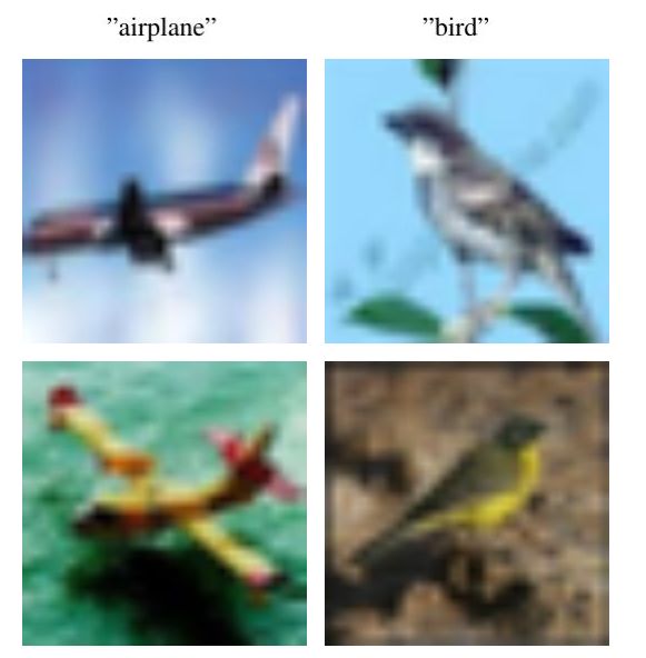
jointly) [3, 4, 14]. An issue that remains is that such ap-
                                                                         proaches are ”free” to learn arbitrary sets of features, and
                                                                         therefore might clusters according to attributes not related
                                                                         to the ground truth labels. To overcome this issue, a promis-
                                                                         ing line of approaches use carefully selected augmentations
                                                                         to remove the nuisance attributes and direct learning to-
                                                                         wards more semantic features [32, 39, 47]. These ideas are
                                                                         often combined with contrastive learning [42]. The work by
                                                                         Van Gansbeke et al. [45] suggested a two stage approach,
                                                                         where features are first learned using a self-supervised task,
                                                                         and then used as a prior for learning the features for cluster-
                                                                         ing. In practice, we often look for clusters which would be
Figure 1. While ground truth CIFAR10 labels associate classes ac-        balanced in size, at least approximately. Many works uti-
cording to object category, clustering according to color or view-       lize an information theoretic criterion to impose such bal-
ing angle can be equally valid. Our ”whitelisting” approach uses         ancing [10, 15, 19].
nouns as the only attributes that can be used for clustering.                Clustering using pretrained features: Some research
                                                                         has also been done on image clustering using features pre-
vanced methods exist for the solution with approximation                 trained on some auxiliary supervised data [12]. While pre-
guarantees, the most popular methods do not scale to our                 trained features are not always applicable, they are often
tasks. Instead, we suggest to solve the optimization task us-            general enough to boost performance on datasets signifi-
ing a more scalable approach, that can be seen as discretized            cantly different than the auxiliary data [23]. However, using
version of K-means                                                       this extra supervision alone does not result in performance
   Using an extensive English dictionary of nouns presents               increase with respect to to the best self-unsupervised meth-
another issue: some uninformative nouns such as ”entity”                 ods. We will also show similar results in this work.
have an embedding similar to a large proportion of images.                   Color name-based features: Color quantization, di-
We propose a unsupervised criterion for selecting a sublist              vides all colors into a discrete number of color groups.
of performant, informative nouns. We extensively evaluate                Although simple K-means approaches are common, it has
our method against top clustering methods that do not use                been argued that grouping according to a list of colors that
our single-noun prior and show that it yields significant per-           have names in the English language provides superior re-
formance gains.                                                          sults to simple clustering only based on the pixel color
   Our main contribution are:                                            statistics [30, 44, 52]. Color name-based identification was
                                                                         further applied to other tasks, such as image classification,
  1. Introducing the single-noun prior to address the prob-              visual tracking and action recognition [43]. As one exam-
     lem of finding meaningful image clusters.                           ple, for the task of person re-identification in surveillance,
                                                                         color names were used as a prior in order to define bet-
  2. Mapping image clustering under the single-noun prior
                                                                         ter similarity metrics, which led to better performance [51],
     to the well-studied facility location problem.
                                                                         and scalability [34]. Our approach can be seen as extending
  3. Suggesting a scalable and empirically effective solu-               these ideas from pixel colors to whole images.
     tion for solving the optimization task.                                 Joint embedding for images and text: Finding the joint
                                                                         embedding of images and text is a long-standing research
  4. Proposing an unsupervised criterion for removing uni-
                                                                         task [31]. A key motivation for looking into such joint em-
     formative nuisance nouns from the noun list.
                                                                         bedding is reducing the requirement for image annotations,
2. Related Works                                                         needed for supervised machine learning classifiers. This
                                                                         can instead be done by utilizing freely-available text cap-
    Self-supervised deep image clustering: Deep features                 tions from the web [21, 35, 38]. It was also suggested that
trained using self-supervised criteria are used extensively              such learned representations can be used for transfer learn-
for image clustering. Early methods learned deep fea-                    ing [11, 28]. Radford et al. [36] presented a new method,
tures using an auto-encoder with a reconstruction constraint             CLIP, that also maps images and sentences into a common
[48, 49]. More recent approaches directly optimize cluster-              space. CLIP was trained using a contrastive objective and
ing objectives during feature learning. Specifically, a com-             provides encoders for images and text. It was shown that
mon approach is to cluster images according to their learned             CLIP can be used for very accurate zero-shot classification
features, and use this approximate clustering for further im-            of standard image datasets, by first mapping all category
provement of the features (this can be done iteratively or               names to embeddings and then for each image choosing

                                                                     2
the category name with the embedding nearest to it. Our clustering according to high-level semantic attributes to-
method relies on the outstanding infrastructure provided wards the goal of clustering by object category. Despite
by CLIP but tackles image clustering rather than zero-shot the more semantic nature of deep features, they still contain
classification. The essential difference is that in CLIP the information on many attributes beyond the object category
set of image labels is provided whereas in clustering the set (including color, texture, pose etc.). Without further super-
of categories is unknown. vision, self-supervised deep features do not perform as well
Uncapacitated facility location problem (UFLP): The as supervised classification methods at separating groups
UFLP problem is a long-studied task in economics, com- according to classes. Although augmentation methods are
puter science, operations research and discrete optimiza- able to remove some attributes from the learned features,
tion. It aims to open a set of facilities, so that they serve all hand-crafting augmentations for all nuisance attributes is a
clients at a minimal cost. Since its introduction in the 1960s daunting (and probably an impossible) task.
(e.g. Kuehn [25]), it attracted many theoretical and heuris-
tic solutions. It has been shown by Guha and Khuller [13] 3.2. The Single-Noun Prior
that the metric UFLP can be solved with a constant approx- Our main proposed idea is to further constrain the clus-
imation guarantee bounded by ρ > 1.463. Different solu- tering task, beyond merely the visual cluster coherence re-
tions methodologies have been applied to the task includ- quirement. Instead of using augmentations as a way of spec-
ing: greedy methods [1], linear-programming with round- ifying the attributes we do not wish to cluster by (”blacklist-
ing [40] and linear-programming primal-dual methods [18]. ing”) - we provide a list of the possible attributes that may
Here, we are concerned with the Uncapcitated K-Facility be used for clustering (”whitelisting”). The whitelisting ap-
Location Problem (UKFLP) [8, 17], which limits the num- proach is more accurate than the blacklisting approach, as
ber of facilities to K. We formulate our optimization ojec- the number of unwanted attributes is potentially infinite and
tive as the UKFLP and use a fast, relaxed variant of the augmentations that remove all those attributes may not be
method of Arya et al. [1]. known.
Our technical approach is called the ”single-noun” prior.
3. Image Clustering with the Single-Noun We first utilize a pre-trained network for mapping images
Prior and nouns into a common feature space. We replace the
within-image coherence requirement, by the requirement
Our goal is to cluster images in a semantically mean- that embeddings of images in a given cluster v ∈ Sk will be
ingful way. We are given NI images, which are mapped similar to the embedding of a single-noun of our dictionary
into feature vectors {v1 ..vNI }, vi ∈ Rd . We further assume w ∈ W describing the cluster. The set of plausible nouns
a list of NW nouns, such that every noun is mapped into (W) can be chosen given the specification of the whitelisted
a vector embedding {u1 ..uNW }, ui ∈ Rd . The list of all attributes.
noun embeddings is denoted as W. The images and nouns In the clustering literature, it is typically required to clus-
are assumed to be embedded in the same feature space, ter a set of images by their object category attribute. We
in the sense that for each image, its nearest noun in fea- observe that the set of object category names is a subset of
ture space provides a good description of the content of the commonly used nouns in the English language. For ex-
the image. We aim to divide the images into K clusters ample, in CIFAR10, the class names are 10 commonly used
{S1 ..SK }. Each cluster should consist of semantically sim- English nouns (”airplane”, ”automobile”, ”bird”, etc.). We
ilar images. We denote the cluster centers by a set of vectors therefore take the entire list of nouns in the WordNet dataset
{c1 ..cK }, ck ∈ Rd . (over 82k nouns) [29] and calculate the embedding for each
noun using the pretrained network, obtaining the noun list
3.1. On the Effectiveness of Features for Clustering W (for details see Sec.5.5).
The above formulation of clustering essentially relies on
3.3. Removing Non-Specific Nouns
the availability of some automatic measure for evaluating
semantic similarity. This is poorly specified as similarity While almost all plausible nouns are contained in the list
may be determined by a large number of attributes such as W, some nouns in the list may have a meaning that is too
object category, color, shape, texture, pose etc. (See Fig.1). general, which may describe images taken out of more than
The choice of image features determines what attributes one groundtruth class, or even be related to all the images in
will be used for measuring similarity. Low level features the dataset. Examples for such nouns are: ’entity’, ’abstrac-
such as raw pixels, color histograms or edge descriptors tion’, ’thing’, ’object’, ’whole’. We would like to filter out
(e.g. SIFT [27] or HOG [9]) are sensitive to low-level at- of our list those nouns that are ambiguous w.r.t. the ground
tributes such as color or simple measures of object pose. truth classes of each dataset, in order to prevent ”false” clus-
More recently, self-supervised deep image features enabled ters. To this end, we first score the ”generality” of each noun
3by calculating the average noun embedding: of a cluster). The optimal assignment should minimize the
sum squared distance between each image and its assigned
1 X
noun. The squared distance between image vi and noun uj
uavg = ui (1)
NW is denoted dij . We can now restate our loss as:
i=1..NW
P
We calculate the generality score s for each noun, as the in- min i∈1..N,j∈1..NW dij xij
xij ,yj
ner product between its embedding ui and the average noun P
s.t. ∀i ∈ 1..N : j∈1..NW xij = 1 (4)
embedding uavg :
P xij ≤ yj
s(ui ) = ui · uavg (2) j∈1..NW yj ≤ K
Where the bottom two constraints limit the number of
We find that this score is indeed higher for the less specific nouns to be at most K.
nouns described earlier. We remove from the list all nouns Solving UKFLP is NP-hard, and the problem of approx-
that have a ”generality score” s higher than some quantile imation algorithms for UKFLP have been studied exten-
level 0 < q ≤ 1, and define the new sublist Wq ⊆ W sively both in terms of complexity and approximation ra-
(|Wq | ≈ q · |W|, where |.| denotes the length of a set). We tio guarantees (see Sec.2). Yet, as the distance matrix dij
choose the quantile q for each dataset using an unsupervised is very large, we could not run the existing solutions at
criterion which considers the balance of the resulting clus- the scale of most of our datasets (there may be as many
ters. Our unsupervised criterion will be detailed in Sec.6. as 82k allowed nouns-”sites” and 260k images-”clients”).
We therefore suggest a relaxed version of the popular Local
3.4. Semantically Coherent Clusters
Search algorithm.
We consider a cluster Sk describable by a single-noun ck
if the embeddings of its associated images are near the em-
4.2. Local Search algorithm
bedding of the noun ck ∈ Wq . We formulate this objective, The Local Search algorithm [1] is an effective, estab-
using the within-cluster sum of squares (WCSS) loss: lished method for solving facility location problems. It
starts with ”forward greedy” initialization: in the first K
PK P 2 steps, we open the new facility (choose a new noun as cen-
min j=1 v∈Sj kv − cj k ter) that minimizes the loss the most among all unopened
{c1 ..cK },{S1 ..SK } (3)
s.t. cj ∈ Wq sites (unselected nouns). For better results, we instead use
Ward’s clustering initialization as described in the end of
The objective is to find assignments {S1 ..Sk } and nouns this section. After initialization, we iteratively perform the
{c1 ..ck } ⊆ Wq , so that the sum of square distances for each following procedure: In each step, we look to swap p of our
cluster between the assigned images and the corresponding selected nouns by p unselected nouns, such that the loss is
noun is minimal. Note that this is not the same as K-means, decreased. If such nouns are found, the swap is applied. We
as the cluster centers are constrained within the discrete set repeat this step until better swaps cannot be found or the
of nouns W whereas in K-means they are unconstrained. maximal number of iterations is reached. The complexity
of this algorithm is O(NI · NW ), making it slow to run even
4. Optimization for our smallest dataset. Therefore, we report the results
only on the STL10 dataset in Sec. 5.4.
4.1. The Uncapacitated Facility Location Problem
4.3. Local Search Location Relaxation Method
We first formalize our optimization problem, by restat-
ing it as an uncapacitated K-facility location problem (UK- As our task is very high-dimensional, running Local
FLP). The UKFLP is a long studied discrete optimization Search (or similar UKFLP algorithms) becomes too slow to
task (see Sec. 2). In the UKFLP task we are asked to ”open” be practical. Therefore, we suggest an alternative, a contin-
K ”facilities” out of a larger set of sites Wq , and assign each uous relaxation approach which is much faster to compute
”client” to one of the K facilities, such that the sum of dis- (with complexity O(NI + NW )). In short, our method first
tances between the ”clients” and their assigned ”facilities” finds the optimal (unconstrained) centered, and than map
is minimal. In our case, the clients are the image embed- them to the allowed set Wq . We iterates the following steps
dings v1 , v2 ..vNI , which are assigned to a set of K noun until convergence:
embeddings selected from the complete list Wq . We look We first assign each of our images v1 ..vN to clusters
to optimize an assignment variable xij ∈ {0, 1} indicat- {S1 ..SK } according to the nearest cluster center (”Voronoi
ing whether the ”client” vi is assigned to the ”facility”, the tessellation”)
noun uj . We also use a variable yj ∈ {0, 1} to determine if
2 2
a facility was opened in site j (if the noun uj is the center Sk0 = {vi | kvi − ck0 k ≤ kvi − ck k , ∀k} (5)
4After assignment, the center locations {c1 ..cK } are set
to be the average feature in each cluster, which minimizes
the WCSS (Eq.3) loss without the constraint. Precisely, we
recompute each cluster center according to the image as-
signment Sk : cj = |S1j | v∈Sj v. However, this is an in-
P
feasible solution as cluster centers will generally not be in
Wq . We therefore replace each cluster center cj with its
nearest neighbour noun in Wq . The result of this step is a
new set of K nouns that form the cluster centers. Instead
of using this new list of nouns as the new cluster centers,
we keep K − p nouns from the previous iteration and select
p nouns from the current set, such that the combined set Figure 2. A qualitative illustration of our results. Left: we present
of nouns decreases the loss in Eq. 3. This is similar to the 3 images of the clusters containing the ’Norwegian elkhound’ dogs
swap in the Local Search algorithm, but differently from it, of the ImageNet Dogs datasets. The results of our method are on
we limit our search space to the new set of K nouns rather top, while the pre-trained visual clustering baseline is at the bot-
than the entire noun list Wq . If no loss decreasing swap is tom. We can see that the cluster computed by our method is more
found, we terminate. invariant to different factors of non-semantic variation while the
Empty and excessively large clusters: In some cases, visual-only baseline clusters similar looking dogs together even if
the discrete nature of the single-noun constraint results in they do not belong to the same species. Right: The noun ’Cer-
berus’ (a mythical 3-headed dog) demonstrates a peculiar failure
excessively large clusters or one of our K centers being
mode of our method w.r.t. to the ImageNet-Dog ground truth
”empty” of samples. In the case of empty clusters, we re-
classes, as it forms clusters containing multiple dogs regardless
place the center location with that of a word which would of their breed.
”attract” more samples. Specifically, we choose that noun
that has the most samples as its nearest neighbours (among
Table 1. Statistics of datasets used in our experiments
those not already is use). To address the problem of ex-
cessively large clusters, we split the samples in that cluster Name Classes Images Dimension
among the nouns in Wq (by distance), and replace the cen- CIFAR-10 10 60,000 32×32×3
ter of the largest cluster with the noun that was chosen by CIFAR-100/20 20 60,000 32×32×3
the largest number of images across the entire dataset. Im- STL-10 10 13,000 96×96×3
ages that only loosely fit the cluster are therefore likely to ImageNet-Dog 15 19,500 2561 ×256×3
be reassigned to other clusters. ImageNet-50 50 65,000 256×256×3
Cluster initialization: We initialize the cluster assign- ImageNet-100 100 130,000 256×256×3
ments using Ward’s clustering on the image embeddings ImageNet-200 200 260,000 256×256×3
v1 , v2 ..vNI . See Sec.5.5 for implementation details and
Sec.5.4 for alternatives.
5. Experiments task, we use the combination of the train and test sets for
We report the results of our method on the datasets that both training and evaluation (a total of 60, 000 images).
are most commonly used for evaluating image clustering, STL10: Another commonly used dataset for image clus-
comparing our results with both fully unsupervised and pre- tering evaluation [7]. Similarly to CIFAR10, we combine
trained clustering methods. We use the three most common the train and test sets. We only use the test set images for
clustering metrics: accuracy (ACC), normalized mutual in- which groundtruth labels exist (a total of 13, 000 images).
formation (NMI) and adjusted rand index (ARI). CIFAR20-100: We use the coarse-grained 20-class ver-
sion of CIFAR100 [24]. we use the combination of the
5.1. Benchmarks train and test sets for both training and evaluation (a total
In this section, we describe the datasets used in our ex- of 60, 000 images).
perimental comparison. The statistics of the datasets are ImageNet dataset: We follow the top performing meth-
summarized in in Tab.1. ods [45] [42], and compare on subsets of the ImageNet-Dog
CIFAR10: The most commonly used dataset for cluster- and ImageNet-50/100/200 derived dataset2 .
ing evaluation [24]. Due to the unsupervised nature of this
1 ImageNet dimension may vary between images 2 https://github.com/vector-1127/DAC/tree/master/Datasets description
5Table 2. Clustering performance comparison on the commonly used benchmarks (%)
CIFAR-10 CIFAR-20/100 STL-10 ImageNet-Dog
NMI ACC ARI NMI ACC ARI NMI ACC ARI NMI ACC ARI
k-means [26] 8.7 22.9 4.9 8.4 13.0 2.8 12.5 19.2 6.1 5.5 10.5 2.0
SC [54] 10.3 24.7 8.5 9.0 13.6 2.2 9.8 15.9 4.8 3.8 11.1 1.3
AE† [2] 23.9 31.4 16.9 10.0 16.5 4.8 25.0 30.3 16.1 10.4 18.5 7.3
DAE† [46] 25.1 29.7 16.3 11.1 15.1 4.6 22.4 30.2 15.2 10.4 19.0 7.8
SWWAE† [55] 23.3 28.4 16.4 10.3 14.7 3.9 19.6 27.0 13.6 9.4 15.9 7.6
GAN† [37] 26.5 31.5 17.6 12.0 15.3 4.5 21.0 29.8 13.9 12.1 17.4 7.8
VAE† [22] 24.5 29.1 16.7 10.8 15.2 4.0 20.0 28.2 14.6 10.7 17.9 7.9
JULE [50] 19.2 27.2 13.8 10.3 13.7 3.3 18.2 27.7 16.4 5.4 13.8 2.8
DEC [48] 25.7 30.1 16.1 13.6 18.5 5.0 27.6 35.9 18.6 12.2 19.5 7.9
DAC [4] 39.6 52.2 30.6 18.5 23.8 8.8 36.6 47.0 25.7 21.9 27.5 11.1
DCCM [47] 49.6 62.3 40.8 28.5 32.7 17.3 37.6 48.2 26.2 32.1 38.3 18.2
IIC [19] - 61.7 - - 25.7 - - 49.9 - - - -
DHOG [10] 58.5 66.6 49.2 25.8 26.1 11.8 41.3 48.3 27.2 - - -
AttentionCluster [32] 47.5 61.0 40.2 21.5 28.1 11.6 44.6 58.3 36.3 28.1 32.2 16.3
MMDC [39] 57.2 70.0 - 25.9 31.2 - 49.8 61.1 - - - -
PICA [16] 59.1 69.6 51.2 31.0 33.7 17.1 61.1 71.3 53.1 35.2 35.2 20.1
SCAN [45] 71.2 81.8 66.5 44.1 42.2 26.7 65.4 75.5 59.0 - - -
MICE [42] 73.5 83.4 69.5 43.0 42.2 27.7 61.3 72.0 53.2 39.4 39.0 24.7
Pretrained 66.8 72.6 57.0 45.1 46.7 26.2 90.2 94.9 88.9 28.4 31.0 17.5
Ours 73.1 85.3 70.2 44.4 43.3 26.3 92.9 97.0 93.4 50.5 55.1 38.1
5.2. Baseline Methods serves as a good comparison point for our method, explor-
ing the utility of our single-noun prior.
Here, we summarize several top performing, relevant
baselines methods. A more general overview of the recently 5.3. Clustering Results
published related works is presented in Sec.2, and a specific
reference for each compared method can be found in Tab.2. We present our clustering results on the described bench-
marks in Tab.2. We compare our results to a large number
SCAN [45]: This method presented a two stage ap- of previous methods using the numbers reported in the cited
proach, which first learns a representation of the data us- paper, when available, and otherwise leave a blank entry.
ing a self-supervised task, and later uses that representation We also present in a comparison against SCAN [45] and
as a prior to optimize the features for clustering. The self- its features on the three random subsets of the ImageNet
supervised feature learning method (namely, SimCLR [5] dataset in Tab.3. We can see that our method achieves the
or MoCo [6]) is used to retrieve the nearest neighbours of highest results on all compared benchmarks.
each image using high level features. The features are then
Noun-based priors: Our single-noun prior improves re-
optimized to satisfy: i) similarity within nearest neighbours
sults significantly for all datasets except CIFAR20-100. The
ii) entropy (uniform distribution among clusters).
pretrained features do not by themselves achieve better clus-
MICE [42]: This method combines a mixture of con- tering accuracy than the self supervised method on most
trastive experts. A gating function is used to weight the ex- benchmarks, demonstrating that our prior is critical. We can
perts based on the the input image. As the gating function see in Tab.5 that the class names of CIFAR10, and the nouns
serves as a soft partitioning of the dataset, each expert is that our method chose as the centers of the corresponding
trained to solve a subtask conditional on the gating function clusters, are closely related. While the class names used by
assignment. the creators of the datasets are only rarely recovered exactly,
Pretrained: We present a naive baseline, based on purely for most classes the cluster centers are a typical subcategory
visual clustering of our image features. The cluster assign- of the original class (”jowett” for car”, ”bulbul” for ”bird”,
ment resulting from this naive method is also used as the ”egyptian cat” for cat”, etc.). A second type of center, is
initialization of our algorithm (see Sec. 4.3). This base- a noun describing a component or an activity strongly as-
line performs better then previously published pretrained sociated with the ”true” class (”ramjet” for ”airplane” or
baselines (Guerinat al. [12] achieves at most 60.8% on CI- ”chukker” for ”horse”). Yet, as can be seen Tab.4, the cen-
FAR10), this is mainly due to the better feature extractor. It ters we found are often on par with the groundtruth class
6Table 3. Clustering performance comparison on randomly selected classes from ImageNet (%)
ImangeNet 50 classes 100 classes 200 classes
NMI ACC ARI NMI ACC ARI NMI ACC ARI
MoCo K-means 77.5 65.9 57.9 76.1 59.7 50.8 75.5 52.5 43.2
SCAN 80.5 75.1 63.5 78.7 66.2 54.4 75.7 56.3 44.1
Pretrained K-means 77.6 66.0 57.6 75.0 61.7 51.9 72.1 53.5 43.8
Pretrained Ward’s 80.4 73.5 61.3 76.2 64.9 52.6 62.0 34.2 23.0
Ours 84.7 82.7 74.4 80.5 73.1 62.8 74.9 59.8 48.6
names in terms of the optimization loss (Eq. 3), and in some line, which utilizes the pretrained visual features alone, only
cases also in terms of accuracy. outperforms other methods on CIFAR20-100 and STL10
datasets, while it underperforms on CIFAR10, ImageNet-
Table 4. Comparison to supervised cluster names (CIFAR10) Dog and the three other ImageNet derived datasets. We
Ours Groundtruth Class names conclude that while pretrained features, when available, are
a strong naive baseline, they are insufficient to convincingly
Acc (%) 85.3 86.0
outperform the top unsupervised methods (e.g. SCAN,
Loss 1.43 1.43
MICE). To evaluate the strength of the CLIP pretrained fea-
tures used in our method, we compare the CLIP encoder to
an ImageNet pretrained wideResnet50x2 [53] and find the
Non-semantic clusters: For CIFAR20-100, our single- the CLIP features compare favourably (Tab.7).
noun prior, not only does not help, but actually impairs the To further understand the importance of our pretrained
results of the pretrained features. A deeper inspection into image features, we compare their performance against the
the 20 aggregated classes of the CIFAR20-100 dataset, finds MoCo features of SCAN [45] (one of the top performing
that the aggregate classes contain mixtures of classes that method) on the ImageNet 50, 100, and 200 benchmarks.
are not strongly semantically related. For example, com- We evaluate clustering using our pretrained visual features
pare ”vehicles 1” aggregate class (”bicycle, bus, motorcy- both with K-means and Ward’s clustering. The results are
cle, pickup truck, train”) to ”vehicles 2” aggregate class reported in Tab.3. We see again that the pretrained visual
(”lawn-mower, rocket, streetcar, tank, tractor”). It is not features of CLIP used in our method by themselves yield
reasonable to assume that ”rocket” should be clustered se- inferior results to the top unsupervised methods. Instead,
mantically, or visually, with ”lawn-mower” rather than with our strong performance is due to the new single-noun prior.
”train”. The single-noun prior therefore does not make Self labeling: SCAN [45] suggested adding an extra
sense in such an artificial setting. On the other hand,for self-labelling step to further boost results. Our method with-
the full CIFAR100 labels (100 classes), which is not com- out self-labeling outperforms SCAN with self-labeling on
monly used for benchmarking clustering, our single-noun most datasets. The exception is CIFAR10 where SCAN
prior does improve the pretrained results from an accuracy with self-labeling achieves 87.6% which is higher than our
of 37.7% to an accuracy of 41.8%. results without self-labeling. We therefore run our method
on CIFAR10 with an extra self-labeling step using Fix-
Table 5. Glossary of CIFAR10 class names and assigned nouns
Match [41], and achieve an accuracy of 92.8%. This suggest
that self-labeling boosts performance independently of the
Classname Cluster Classname Cluster
base clustering method.
airplane ramjet dog maltese dog
truck milk float frog barking frog 5.4. Ablation studies
automobile jowett ship pilot boat Facility location optimization methods: As explained
horse chukker cat egyptian cat in Sec.4.3, our optimization method can be viewed as a re-
bird bulbul deer pere david’s deer laxed version of the Local Search algorithm. We initially
ignore the discrete constraint, optimize the centers loca-
tions, and then apply a ”rounding” process. For STL10
Comparison of the underlying features: Our setting - our smallest datasets, we were able to run the original
assumes the availability of two components not assumed Local Search algorithm with a single swap in each step
by previous methods: pretrained visual features and a com- (also known as the Portioning around Medoids algorithm
mon feature space for text and images. Our pretrained base- or PAM). As can be seen in Tab.6, PAM reaches compara-
7ble losses to our method, both methods achieve loss values photo of a ***” prompt, where *** is a single-noun from
that are lower than the loss with the groundtruth nouns as our dictionary.
center (Lgt = 1.48). These metrics suggest that both meth- Feature normalization: Following CLIP [36], we L2
ods can effectively optimize the objective, and differences normalize our image and text features at initialization, and
in results are due to the stochastic nature of the methods and at each step of our algorithm. Working with normalized
the fact the objective does not perfectly specify the full im- features implies that the Euclidean distance used throughout
age classification task. Yet, the time complexity of PAM is our algorithm is equivalent to the cosine similarity metric.
significantly greater than that of our relaxed version. Metrics: For the NMI and accuracy score we used the
It was theoretically shown that the approximation bound code3 provided by Shiran et. al. [39]. For the ARI score,
on the loss acieved by PAM improves as the number of we use the adjusted rand score function from scikit-learn
swaps per-iterations p is increased. On the other hand, the library [33].
runtime complexity is exponential in p. We explored the Nearest neighbours retrieval: For nearest neighbours
performance of our method with all possible numbers of retrieval and plain K-means clustering we use faiss library
swap. Different choices of the number of swaps p achieved [20].
very similar accuracy, suggesting the minima we find typi- Clustering initialization: For Ward’s agglomerative
cally are unaffected by it. clustering we use scikit-learn library [33].
Self-labelling: We use the FixMatch [41] PyTorch im-
Table 6. Comparison between PAM and our method (STL10) plementation, initializing it with the 100 most confident
Ours PAM samples in each of our clusters.
Acc (%) 96.8 96.3
Loss 1.47 1.47
6. Analysis
The expressivity of our model: We report the accuracy
on CIFAR10 using the groundtruth class names as the nouns
Design choices: In Tab.7 we compare different initial- (See Tab.4). We see that the solution we found for CIFAR10
ization options of our method. Ward’s agglomerative clus- is close to optimal zero-shot classification result. We note
tering initialization is better than K-means clustering, prob- that the while the CLIP [36] paper reports better classifica-
ably as K-means tends to ”get stuck” in local minima. tion results, it uses extensive prompts engineering which is
beyond the scope of this paper. Furthermore, as the ground
Table 7. Comparison of initialization methods (CIFAR10) truth results actually achieve a similar loss to ours, a further
improvement of our method is more likely to come from
CLIP-Ward CLIP-Kmeans ResNet-Ward extending the expressivity of our model rather than a better
optimization process.
Acc (%) 72.6 69.4 64.6
Filtering our nouns list: Before running the algorithm,
we filter out nouns whose ”generality” score is above some
quantile q, as mentioned in Sec.3.3. To do so in unsuper-
vised way, we try a set of values for q (see implementation
5.5. Implementation details
details 5.5), and run our algorithm with each them. For each
Optimization: We run our algorithm with p = #classes 2 value of q, we obtain cluster assignments, and calculate the
swaps per iteration. For every experiment we run our algo- entropy. We choose to use the q value for which our noun
rithm for 30 iterations which was checked to be enough for list Wq gives the most balanced clustering for each dataset,
convergence for all datasets. We note that in our variation of measured as the highest entropy cluster assignment. For il-
relaxed Local Search, we randomly replace p of our centers lustration, in Fig.3 we show that the accuracy of our cluster-
with the new ones, and execute the replacement if the loss ing, and the entropy value are correlated for different quan-
with the new centers is lower. tile threshold q.
Dictionary: For each dataset we try different quantile
levels q of ”generality” filtering. We use 20 q values be- 7. Conclusion
tween 0.05, and 1 in 0.05 intervals and choose between
We presented the ”single-noun” prior for biasing cluster-
them using our unsupervised criterion as we will show in
ing methods towards more semantic clusters. The task was
Sec.6.
shown to be mathematically equivalent to the uncapcitated
Features: We used the CLIP [36] pretrained model for
K-facility location problem, and we suggested an efficient
our pretrained visual and text features. For the visual fea-
optimization method for solving it. While our approach
tures we choose the ViT-B-32 network. For the text features
we use the suggested transformer, applied with a ”This is a 3 https://github.com/guysrn/mmdc/blob/main/utils/metrics.py
8Figure 3. CIFAR10 Accuracy vs. Unsupervised criterion Proceedings of the fourteenth international conference on
artificial intelligence and statistics, pages 215–223. JMLR
Workshop and Conference Proceedings, 2011.
[8] Gérard Cornuéjols, George Nemhauser, and Laurence
Wolsey. The uncapicitated facility location problem. Tech-
nical report, Cornell University Operations Research and In-
dustrial Engineering, 1983.
[9] Navneet Dalal and Bill Triggs. Histograms of oriented gra-
dients for human detection. In 2005 IEEE computer soci-
ety conference on computer vision and pattern recognition
(CVPR’05), volume 1, pages 886–893. Ieee, 2005.
[10] Luke Nicholas Darlow and Amos Storkey. Dhog: Deep hier-
archical object grouping. arXiv preprint arXiv:2003.08821,
2020.
[11] Karan Desai and Justin Johnson. Virtex: Learning visual
representations from textual annotations. arXiv preprint
arXiv:2006.06666, 2020.
[12] Joris Guérin, Stephane Thiery, Eric Nyiri, Olivier Gibaru,
is very effective, we acknowledge that not all clusters are and Byron Boots. Combining pretrained cnn feature extrac-
defined by nouns. Other datasets classes, such as ones in tors to enhance clustering of complex natural images. Neu-
rocomputing, 423:551–571, 2021.
which classes are defined by activities, might benefit from
[13] Sudipto Guha and Samir Khuller. Greedy strikes back: Im-
other lists, for example those of single-adjectives. Explor-
proved facility location algorithms. Journal of algorithms,
ing this setting is left for future work. 31(1):228–248, 1999.
[14] Philip Haeusser, Johannes Plapp, Vladimir Golkov, Elie Al-
Acknowledgements jalbout, and Daniel Cremers. Associative deep clustering:
Training a classification network with no labels. In German
This work was partly supported by the Federmann Cy- Conference on Pattern Recognition, pages 18–32. Springer,
ber Security Research Center in conjunction with the Israel 2018.
National Cyber Directorate. [15] Weihua Hu, Takeru Miyato, Seiya Tokui, Eiichi Matsumoto,
and Masashi Sugiyama. Learning discrete representations
References via information maximizing self-augmented training. In In-
ternational Conference on Machine Learning, pages 1558–
[1] Vijay Arya, Naveen Garg, Rohit Khandekar, Adam Meyer-
1567. PMLR, 2017.
son, Kamesh Munagala, and Vinayaka Pandit. Local search
[16] Jiabo Huang, Shaogang Gong, and Xiatian Zhu. Deep se-
heuristics for k-median and facility location problems. SIAM
mantic clustering by partition confidence maximisation. In
Journal on computing, 33(3):544–562, 2004.
Proceedings of the IEEE/CVF Conference on Computer Vi-
[2] Yoshua Bengio, Pascal Lamblin, Dan Popovici, Hugo sion and Pattern Recognition, pages 8849–8858, 2020.
Larochelle, et al. Greedy layer-wise training of deep net- [17] Kamal Jain, Mohammad Mahdian, and Amin Saberi. A new
works. Advances in neural information processing systems, greedy approach for facility location problems. In Proceed-
19:153, 2007. ings of the thiry-fourth annual ACM symposium on Theory
[3] Mathilde Caron, Piotr Bojanowski, Armand Joulin, and of computing, pages 731–740, 2002.
Matthijs Douze. Deep clustering for unsupervised learning [18] Kamal Jain and Vijay V Vazirani. Approximation algorithms
of visual features. In Proceedings of the European Confer- for metric facility location and k-median problems using the
ence on Computer Vision (ECCV), pages 132–149, 2018. primal-dual schema and lagrangian relaxation. Journal of the
[4] Jianlong Chang, Lingfeng Wang, Gaofeng Meng, Shiming ACM (JACM), 48(2):274–296, 2001.
Xiang, and Chunhong Pan. Deep adaptive image cluster- [19] Xu Ji, João F Henriques, and Andrea Vedaldi. Invariant in-
ing. In Proceedings of the IEEE international conference on formation clustering for unsupervised image classification
computer vision, pages 5879–5887, 2017. and segmentation. In Proceedings of the IEEE/CVF Inter-
[5] Ting Chen, Simon Kornblith, Mohammad Norouzi, and Ge- national Conference on Computer Vision, pages 9865–9874,
offrey Hinton. A simple framework for contrastive learning 2019.
of visual representations. In International conference on ma- [20] Jeff Johnson, Matthijs Douze, and Hervé Jégou. Billion-
chine learning, pages 1597–1607. PMLR, 2020. scale similarity search with gpus. IEEE Transactions on Big
[6] Xinlei Chen, Haoqi Fan, Ross Girshick, and Kaiming He. Data, 2019.
Improved baselines with momentum contrastive learning. [21] Armand Joulin, Laurens Van Der Maaten, Allan Jabri, and
arXiv preprint arXiv:2003.04297, 2020. Nicolas Vasilache. Learning visual features from large
[7] Adam Coates, Andrew Ng, and Honglak Lee. An analysis of weakly supervised data. In European Conference on Com-
single-layer networks in unsupervised feature learning. In puter Vision, pages 67–84. Springer, 2016.
9[22] Diederik P Kingma and Max Welling. Auto-encoding varia- tional generative adversarial networks. arXiv preprint
tional bayes. arXiv preprint arXiv:1312.6114, 2013. arXiv:1511.06434, 2015.
[23] Simon Kornblith, Jonathon Shlens, and Quoc V Le. Do [38] Mert Bulent Sariyildiz, Julien Perez, and Diane Larlus.
better imagenet models transfer better? In Proceedings of Learning visual representations with caption annotations.
the IEEE/CVF Conference on Computer Vision and Pattern arXiv preprint arXiv:2008.01392, 2020.
Recognition, pages 2661–2671, 2019. [39] Guy Shiran and Daphna Weinshall. Multi-modal deep clus-
[24] Alex Krizhevsky, Geoffrey Hinton, et al. Learning multiple tering: Unsupervised partitioning of images. arXiv preprint
layers of features from tiny images. 2009. arXiv:1912.02678, 2019.
[25] Alfred A Kuehn and Michael J Hamburger. A heuristic [40] David B Shmoys, Éva Tardos, and Karen Aardal. Approxi-
program for locating warehouses. Management science, mation algorithms for facility location problems. In Proceed-
9(4):643–666, 1963. ings of the twenty-ninth annual ACM symposium on Theory
[26] Stuart Lloyd. Least squares quantization in pcm. IEEE trans- of computing, pages 265–274, 1997.
actions on information theory, 28(2):129–137, 1982. [41] Kihyuk Sohn, David Berthelot, Chun-Liang Li, Zizhao
[27] David G Lowe. Object recognition from local scale-invariant Zhang, Nicholas Carlini, Ekin D Cubuk, Alex Kurakin, Han
features. In Proceedings of the seventh IEEE international Zhang, and Colin Raffel. Fixmatch: Simplifying semi-
conference on computer vision, volume 2, pages 1150–1157. supervised learning with consistency and confidence. arXiv
Ieee, 1999. preprint arXiv:2001.07685, 2020.
[28] Dhruv Mahajan, Ross Girshick, Vignesh Ramanathan, [42] Tsung Wei Tsai, Chongxuan Li, and Jun Zhu. Mi{ce}: Mix-
Kaiming He, Manohar Paluri, Yixuan Li, Ashwin Bharambe, ture of contrastive experts for unsupervised image cluster-
and Laurens Van Der Maaten. Exploring the limits of weakly ing. In International Conference on Learning Representa-
supervised pretraining. In Proceedings of the European Con- tions, 2021.
ference on Computer Vision (ECCV), pages 181–196, 2018.
[43] Joost Van De Weijer and Fahad Shahbaz Khan. An overview
[29] George A Miller. Wordnet: a lexical database for english.
of color name applications in computer vision. In Interna-
Communications of the ACM, 38(11):39–41, 1995.
tional Workshop on Computational Color Imaging, pages
[30] Aleksandra Mojsilovic. A computational model for color 16–22. Springer, 2015.
naming and describing color composition of images. IEEE
[44] Joost Van De Weijer, Cordelia Schmid, Jakob Verbeek, and
Transactions on Image processing, 14(5):690–699, 2005.
Diane Larlus. Learning color names for real-world applica-
[31] Yasuhide Mori, Hironobu Takahashi, and Ryuichi Oka.
tions. IEEE Transactions on Image Processing, 18(7):1512–
Image-to-word transformation based on dividing and vector
1523, 2009.
quantizing images with words. In First international work-
shop on multimedia intelligent storage and retrieval manage- [45] Wouter Van Gansbeke, Simon Vandenhende, Stamatios
ment, pages 1–9. Citeseer, 1999. Georgoulis, Marc Proesmans, and Luc Van Gool. Scan:
Learning to classify images without labels. In European
[32] Chuang Niu, Jun Zhang, Ge Wang, and Jimin Liang. Gat-
Conference on Computer Vision, pages 268–285. Springer,
cluster: Self-supervised gaussian-attention network for im-
2020.
age clustering. In European Conference on Computer Vision,
pages 735–751. Springer, 2020. [46] Pascal Vincent, Hugo Larochelle, Isabelle Lajoie, Yoshua
[33] Fabian Pedregosa, Gaël Varoquaux, Alexandre Gramfort, Bengio, Pierre-Antoine Manzagol, and Léon Bottou.
Vincent Michel, Bertrand Thirion, Olivier Grisel, Mathieu Stacked denoising autoencoders: Learning useful represen-
Blondel, Peter Prettenhofer, Ron Weiss, Vincent Dubourg, tations in a deep network with a local denoising criterion.
et al. Scikit-learn: Machine learning in python. the Journal Journal of machine learning research, 11(12), 2010.
of machine Learning research, 12:2825–2830, 2011. [47] Jianlong Wu, Keyu Long, Fei Wang, Chen Qian, Cheng Li,
[34] Raphael Prates, Cristianne RS Dutra, and William Robson Zhouchen Lin, and Hongbin Zha. Deep comprehensive cor-
Schwartz. Predominant color name indexing structure for relation mining for image clustering. In Proceedings of the
person re-identification. In 2016 IEEE International Con- IEEE/CVF International Conference on Computer Vision,
ference on Image Processing (ICIP), pages 779–783. IEEE, pages 8150–8159, 2019.
2016. [48] Junyuan Xie, Ross Girshick, and Ali Farhadi. Unsupervised
[35] Ariadna Quattoni, Michael Collins, and Trevor Darrell. deep embedding for clustering analysis. In International
Learning visual representations using images with captions. conference on machine learning, pages 478–487. PMLR,
In 2007 IEEE Conference on Computer Vision and Pattern 2016.
Recognition, pages 1–8. IEEE, 2007. [49] Bo Yang, Xiao Fu, Nicholas D Sidiropoulos, and Mingyi
[36] Alec Radford, Jong Wook Kim, Chris Hallacy, Aditya Hong. Towards k-means-friendly spaces: Simultaneous deep
Ramesh, Gabriel Goh, Sandhini Agarwal, Girish Sastry, learning and clustering. In international conference on ma-
Amanda Askell, Pamela Mishkin, Jack Clark, et al. Learn- chine learning, pages 3861–3870. PMLR, 2017.
ing transferable visual models from natural language super- [50] Jianwei Yang, Devi Parikh, and Dhruv Batra. Joint unsuper-
vision. Image, 2:T2, 2021. vised learning of deep representations and image clusters. In
[37] Alec Radford, Luke Metz, and Soumith Chintala. Un- Proceedings of the IEEE conference on computer vision and
supervised representation learning with deep convolu- pattern recognition, pages 5147–5156, 2016.
10[51] Yang Yang, Jimei Yang, Junjie Yan, Shengcai Liao, Dong
Yi, and Stan Z Li. Salient color names for person re-
identification. In European conference on computer vision,
pages 536–551. Springer, 2014.
[52] Lu Yu, Lichao Zhang, Joost van de Weijer, Fahad Shahbaz
Khan, Yongmei Cheng, and C Alejandro Parraga. Beyond
eleven color names for image understanding. Machine Vision
and Applications, 29(2):361–373, 2018.
[53] Sergey Zagoruyko and Nikos Komodakis. Wide residual net-
works. arXiv preprint arXiv:1605.07146, 2016.
[54] Lihi Zelnik-Manor and Pietro Perona. Self-tuning spectral
clustering, 2004. Advances in Neural Information Process-
ing Systems, 17, 2005.
[55] Junbo Zhao, Michael Mathieu, Ross Goroshin, and Yann
Lecun. Stacked what-where auto-encoders. arXiv preprint
arXiv:1506.02351, 2015.
11You can also read