Topological Information Retrieval with Dilation-Invariant Bottleneck Comparative Measures
←
→
Page content transcription
If your browser does not render page correctly, please read the page content below
Topological Information Retrieval with Dilation-Invariant
                                          Bottleneck Comparative Measures
                                          Athanasios Vlontzos1,∗,† , Yueqi Cao2,∗ , Luca Schmidtke1 , Bernhard Kainz1 , and Anthea Monod2,†

                                          1 Department of Computing, Imperial College London, UK
                                          2 Department of Mathematics, Imperial College London, UK

                                          * These authors contributed equally to this work
                                          † Corresponding e-mail: athanasios.vlontzos14@imperial.ac.uk, a.monod@imperial.ac.uk
arXiv:2104.01672v2 [stat.ML] 1 Aug 2021

                                          Abstract
                                          Appropriately representing elements in a database so that queries may be accurately matched is a central
                                          task in information retrieval; recently, this has been achieved by embedding the graphical structure of the
                                          database into a manifold in a hierarchy-preserving manner using a variety of metrics. Persistent homology is
                                          a tool commonly used in topological data analysis that is able to rigorously characterize a database in terms
                                          of both its hierarchy and connectivity structure. Computing persistent homology on a variety of embedded
                                          datasets reveals that some commonly used embeddings fail to preserve the connectivity. We show that those
                                          embeddings which successfully retain the database topology coincide in persistent homology by introducing
                                          two dilation-invariant comparative measures to capture this effect: in particular, they address the issue of
                                          metric distortion on manifolds. We provide an algorithm for their computation that exhibits greatly reduced
                                          time complexity over existing methods. We use these measures to perform the first instance of topology-
                                          based information retrieval and demonstrate its increased performance over the standard bottleneck distance
                                          for persistent homology. We showcase our approach on databases of different data varieties including text,
                                          videos, and medical images.

                                          Keywords: Bottleneck distance; Database embeddings; Dilation invariance; Information retrieval; Persis-
                                          tent homology.

                                          1    Introduction
                                          The fundamental problem of information retrieval (IR) is to find the most related elements in a database
                                          for a given query. Given that queries often comprise multiple components, candidate matches must satisfy
                                          multiple conditions, which gives rise to a natural hierarchy and connectivity structure of the database. This
                                          structure is important to maintain in performing IR. For example, when searching for a person named “John
                                          Smith” in a database, the search algorithm may search among all entries with the last name “Smith” and
                                          then among those entries, search for those with the first name “John.” Additionally, cycles and higher order
                                          topological features in the database correspond to entries that are directly related and may be, for instance,
                                          suitable alternative matches: as an example, in online shopping, when recommendations for other products
                                          are proposed as either alternative or complementary to the original query (i.e., they are recommended for their
                                          connection). The hierarchical and connectivity structure of databases motivates the study of the topology of
                                          databases. Topology characterizes abstract geometric properties of a set or space, such as its connectivity.
                                          Prior work has used point-set topology to describe databases (Egghe, 1998; Clementini et al., 1994; Egghe
                                          and Rousseau, 1998; Everett and Cater, 1992a). In this paper, we explore an alternative approach based on
                                          algebraic topology.
                                              Topological data analysis (TDA) has recently been utilized in many fields and yielded prominent results,
                                          including imaging (Crawford et al., 2020; Perea and Carlsson, 2014), biology and neuroscience (Anderson
                                          et al., 2018; Aukerman et al., 2020), materials science (Hiraoka et al., 2016; Hirata et al., 2020), and sensor
                                          networks (Adams and Carlsson, 2015; de Silva and Ghrist, 2006). TDA has also recently gained interest
                                          in machine learning (ML) in many contexts, including loss function construction, generative adversarial
                                          networks, deep learning and deep neural networks, representation learning, kernel methods, and autoencoders
(Brüel-Gabrielsson et al., 2019; Hofer et al., 2017, 2019; Hu et al., 2019; Moor et al., 2020; Reininghaus et al.,
2015).
Persistent homology is a fundamental TDA methodology that extracts the topological features of a dataset
in an interpretable, lower-dimensional representation (Edelsbrunner et al., 2000; Frosini and Landi, 1999;
Zomorodian and Carlsson, 2005). Persistent homology is particularly amenable to data analysis since it
produces a multi-scale summary, known as a persistence diagram, which tracks the presence and evolution
of topological features. Moreover, persistent homology is robust to noise and allows for customization of the
chosen metric, making it applicable to a wide range of applications (Cohen-Steiner et al., 2007).
In this paper, we apply persistent homology to the setting of database queries and IR to understand the
structure and connectivity of databases, which are possibly unknown, but may be summarized using topology.
Persistent homology, in particular, provides an intuition on the prominence of each topological feature within
the dataset. We show that the topological characteristics of a hierarchical and interdependent database
structure are preserved in some commonly used embeddings and not in others. Moreover, we find that
there is a high degree of similarity between topology-preserving embeddings. To capture and quantify this
similarity, we introduce the dilation-invariant bottleneck dissimilarity and distance for persistent homology
to mitigate the issue of metric distortion in manifold embeddings. We use these measures in an exploratory
analysis as well as to perform an IR task on real databases, where we show increased performance over the
standard bottleneck distance for persistent homology. To the best of our knowledge, this is the first instance
where TDA tools are used to describe database representations and to perform IR.
The remainder of this paper is structured as follows. We close this first Section 1 with a discussion
on related work. We then present the key ideas behind TDA in Section 2 and introduce our dilation-
invariant bottleneck comparative measures. In Section 3 we present efficient methods to compute both
dilation-invariant bottleneck comparative measures and prove results on the correctness and complexity of
our algorithms. In particular, we show that the time complexity of our algorithm to compute the dilation-
invariant bottleneck distance is vastly more efficient than existing work that computes the related shift-
invariant bottleneck distance. In Section 4, we present two applications to data: an exploratory data
analysis on database representations and an IR task by classification. We conclude in Section 5 with some
thoughts from our study and directions for future research.
Related Work. IR has been a topic of active research, particularly within the natural language processing
(NLP) community. Document retrieval approaches have proposed a sequence-to-sequence model to increase
performance in cross-lingual IR (Boudin et al., 2020; Liu et al., 2020). A particularly interesting challenge in
IR in NLP is word-sense disambiguation, where the closest meaning of a word given a context is retrieved.
Approaches to this problem have been proposed where the power of large language models is leveraged to
embed not only words but also their contexts; the embeddings are further enriched with other sources, such
as the WordNet hierarchical structure, before comparing the queries to database elements (Bevilacqua and
Navigli, 2020; Scarlini et al., 2020; Yap et al., 2020). Inference is usually done either using cosine similarity
as a distance function or through a learned network.
IR also arises in contexts other than NLP, such as image and video retrieval (Long et al., 2020). Image
and video retrieval challenges, such as those proposed by Heilbron et al. (2015); Google (2018), have inspired
the development of a wide variety of techniques.
Topology-enabled IR. Prior work that adapts topology to IR proposes topological analysis systems in the
setting of point-set topology: these models are theoretical, and use separation axioms in topological spaces
to describe the restriction on topologies to define a threshold for retrieval (Egghe, 1998; Clementini et al.,
1994; Egghe and Rousseau, 1998; Everett and Cater, 1992b,a). A tool set based on point-set topology has
also been proposed to improve the performance of enterprise-related document retrieval (Deolalikar, 2015).
More recently, and relevant to the task of IR, Aloni et al. (2021) propose a method that jointly implements
geometric and topological concepts—including persistent homology—to build a representation of hierarchical
databases. Our approach is in contrast to this work and other data representation or compression tasks,
such as that by Moor et al. (2020), in the sense that we do not seek to impose geometric or topological
structure on a database nor do we explicitly enforce a topological constraint. Rather, we seek to study its
preconditioned hierarchical structure using persistent homology and use this information to perform IR.
22 Topological Data Analysis
TDA adapts algebraic topology to data. Classical topology studies features of spaces that are invariant
under smooth transformations (e.g., “stretching” without “tearing”). A prominent example for such features
is k-dimensional holes, where dimension 0 corresponds to connected components, dimension 1 to cycles,
dimension 2 to voids, and so on. Homology is a theoretical concept that algebraically identifies and counts
these features. The crux of topological data analysis is that topology captures meaningful aspects of the
data, while algebraicity lends interpretability and computational feasibility.
2.1 Persistent Homology
Persistent homology adapts homology to data and outputs a set of topological descriptors that summarizes
topological information of the dataset. Data may be very generally represented as a finite point cloud,
which is a collection of points sampled from an unknown manifold, together with some similarity measure
or metric. Point clouds may therefore be viewed as finite metric spaces. Persistent homology assigns a
continuous, parameterized sequence of nested skeletal structures to the point cloud according to a user-
specified proximity rule. The appearance and dissipation of holes in this sequence is tracked, providing
a concise summary of the presence of homological features in the data at all resolutions. We now briefly
formalize these technicalities; a complete discussion with full details can be found in the literature on applied
and computational topology (e.g., Carlsson (2009); Ghrist (2008); Edelsbrunner and Harer (2008)).
Although the underlying idea of homology is intuitive, computing homology can be challenging. One
convenient workaround is to study a discretization of the topological space as a union of simpler building
blocks assembled in a combinatorial manner. When the building blocks are simplices (e.g., vertices, lines,
triangles, and higher-dimensional facets), the skeletonized version of the space as a union of simplices is a
simplicial complex, and the resulting homology theory is simplicial homology, for which there exist efficient
computational algorithms (see, e.g., Munkres (2018) for a background reference on algebraic topology). Thus,
in this paper, we will use simplicial homology over a field to study a finite topological space X; (X, dX ) is
therefore a finite metric space.
A k-simplex is the convex hull of k+1 affinely independent points x0 , x1 , . . . , xk , denoted by [x0 , x1 , . . . , xk ];
a set of k-simplices forms a simplicial complex K. Simplicial homology is based on simplicial k-chains, which
are linear combinations of k-simplices in finite K over a field F. A set of k-chains thus defines a vector space
Ck (K).
Definition 1. The boundary operator ∂k : Ck (K) → Ck−1 (K) maps to lower dimensions of the vector
Pk
spaces by sending simplices [x0 , x1 , . . . , xk ] 7→ i=0 (−1)i [x0 , . . . , x̂i , . . . , xk ] with linear extension, where x̂i
indicates that the ith element is dropped. Bk (K) := im ∂k+1 is the set of boundaries; Zk (K) := ker ∂k is
the set of cycles. The kth homology group of K is the quotient group Hk (K) := Zk (K)/Bk (K).
Homology documents the structure of K, which is a finite simplicial complex representation of a topo-
logical space X. Simplicial complexes K may be constructed according to various assembly rules, which
give rise to different complex types. In this paper, we work with the Vietoris–Rips (VR) complexes and
filtrations.
Definition 2. Let (X, dX ) be a finite metric space, let r ∈ R≥0 . The Vietoris–Rips complex of X is the
simplicial complex with vertex set X where {x0 , x1 , . . . , xk } spans a k-simplex if and only if the diameter
d(xi , xj ) ≤ r for all 0 ≤ i, j ≤ k.
A filtration of a finite simplicial complex K is a sequence of nested subcomplexes K0 ⊆ K1 ⊆ · · · ⊆ Kt =
K; a simplicial complex K that can be constructed from a filtration is a filtered simplicial complex. In this
paper, filtrations are indexed by a continuous parameter r ∈ [0, t]; setting the filtration parameter to be the
diameter r of a VR complex yields the Vietoris–Rips filtration.
Persistent homology computes homology in a continuous manner when the simplicial complex evolves
continuously over a filtration.
Definition 3. Let K be a filtered simplicial complex. The kth persistence module derived in homology of
K is the collection PHk (K) := {Hk (Kr )}0≤r≤t , together with associated linear maps {ϕr,s }0≤rFigure 1: Illustration of a VR filtration and persistent homology. For a sample of points, a closed metric ball
is grown around each point. The radius of the balls is the VR threshold, r. Points are connected by an edge
whenever two balls have a non-empty intersection; k-simplices are spanned for intersections of k balls. As
r grows, the collection of k-simplices evolves, yielding a VR filtration. The topology of the VR filtration is
tracked in terms of the homological features (connected components, cycles, voids) that appear (are “born”),
evolve, and disappear (“die”) as r grows, and documented in a persistence diagram (right-most). In this
figure, red points correspond to H0 homology, or connected components, and green points correspond to H1
homology, or cycles.
Persistent homology, therefore, contains information not only on the individual spaces {Kr } but also
on the mappings between every pair Kr and Ks where r ≤ s. Persistent homology keeps track of the
continuously evolving homology of X across all scales as topological features (captured by simplices) appear,
evolve, and disappear as the filtered simplicial complex K evolves with the filtration parameter r.
Persistent homology outputs a collection of intervals where each interval represents a topological feature
in the filtration; the left endpoint of the interval signifies when each feature appears (or is “born”), the right
endpoint signifies when the feature disappears or merges with another feature (“dies”), and the length of the
interval corresponds to the feature’s “persistence.” Each interval may be represented as a set of ordered pairs
and plotted as a persistence diagram. A persistence diagram of a persistence module, therefore, is a multiset
of points in R2 . Typically, points located close to the diagonal in a persistence diagram are interpreted as
topological “noise” while those located further away from the diagonal can be seen as “signal.” The distance
from a point on the persistence diagram to its projection on the diagonal is a measure of the topological
feature’s persistence. Figure 1 provides an illustrative depiction of a VR filtration and persistence diagram.
In real data applications (and in this paper), persistence diagrams are finite.
2.2 Distances Between Persistence Diagrams
The set of all persistence diagrams can be endowed with various distance measures; under mild regularity
conditions (of local finiteness of persistence diagrams), it is a rigorous metric space. The bottleneck distance
measures distances between two persistence diagrams as a minimal matching between the two diagrams,
allowing points to be matched with the diagonal ∆, which is the multiset of all (x, x) ∈ R2 with infinite
multiplicity, or the set of all zero-length intervals.
Definition 4. Let M be the space of all finite metric spaces. Let Dgm(X, dX ) be the persistence diagram
corresponding to the VR persistent homology of (X, dX ). Let D = {Dgm(X, dX ) | (X, dX ) ∈ M} be the
space of persistence diagrams of VR filtrations for finite metric spaces in M. The bottleneck distance on D
is given by
d∞ (Dgm(X, dX ), Dgm(Y, dY )) = inf sup kx − γ(x)k∞ ,
γ x∈Dgm(X,d )
X
where γ is a multi-bijective matching of points between Dgm(X, dX ) and Dgm(Y, dY ).
The fundamental stability theorem in persistent homology asserts that small perturbations in input data
will result in small perturbations in persistence diagrams, measured by the bottleneck distance (Cohen-
4Steiner et al., 2007). This result together with its computational feasibility renders the bottleneck distance
the canonical metric on the space of persistence diagrams for approximation studies in persistent homology.
Persistence diagrams, however, are not robust to the scaling of input data and metrics: the same point
cloud measured by the same metric in different units results in different persistence diagrams with a poten-
tially large bottleneck distance between them. One way that this discrepancy has been previously addressed
is to study filtered complexes on a log scale, such as in Bobrowski et al. (2017); Buchet et al. (2016); Chazal
et al. (2013). In these works, the persistence of a point in the persistence diagram (in terms of its distance
to the diagonal) is based on the ratio of birth and death times, which alleviates the issue of artificial infla-
tion in persistence arising from scaling. Nevertheless, these approaches fail to recognize when two diagrams
arising from the same input data measured by the same metric but in different units should coincide. The
shift-invariant bottleneck distance proposed by Sheehy et al. (2018) addresses this issue by minimizing over
all shifts along the diagonal, which provides scale invariance for persistence diagrams.
A further challenge is to recognize when the persistent homology of an input dataset is computed with
two different metrics and we would like to deduce that the topology the dataset is robust to the choice of
metric. Neither log-scale persistence nor the shift-invariant bottleneck distance is able to recognize when two
persistence diagrams are computed from the same dataset but with different metrics. We therefore introduce
the dilation-invariant bottleneck dissimilarity which mitigates this effect of metric distortion on persistence
diagrams. The dilation-invariant bottleneck dissimilarity erases the effect of scaling between metrics used to
construct the filtered simplicial complex and instead focuses on the topological structure of the point cloud.
2.3 Dilation-Invariant Bottleneck Comparison Measures
The dilation-invariant bottleneck comparison measures we propose are motivated by the shift-invariant
bottleneck distance proposed by Sheehy et al. (2018), which we now briefly overview. Let F = {f : X → R}
be the space of continuous tame functions over a fixed triangulable topological space X, equipped with
supremum metric dF (f, g) = supx |f (x) − g(x)|. Define an isometric action of R on F by
R×F →F
(c, f ) 7→ f + c.
The resulting quotient space F = F/R is a metric space with the quotient metric defined by
dF ([f ], [g]) = inf sup |f (x) + c − g(x)| = inf dF (f + c, g).
c∈R x∈X c∈R
Let D∞ = {Dgm(f ) | f ∈ F} be the space of persistence diagrams of functions in F, equipped with the
standard bottleneck distance. Similarly, we can define the action
R × D∞ → D∞
(c, Dgm(f )) 7→ Dgm(f + c).
The resulting quotient space D∞ = D/R is a metric space with the quotient metric defined by
dS ([Dgm(f )], [Dgm(g)]) = inf d∞ (Dgm(f + c), Dgm(g)). (1)
c∈R
The quotient metric dS is precisely the shift-invariant bottleneck distance: effectively, it ignores translations
of persistence diagrams, meaning that two persistence diagrams computed from the same metric but measured
in different units will measure a distance of zero with the shift-invariant bottleneck distance.
From this construction, we derive the dilation-invariant dissimilarity and distance in the following two
ways. In a first instance, we replace shifts of tame functions by dilations of finite metric spaces. A critical
difference between our setting and that of the shift-invariant bottleneck distance is that dilation is not an
isometric action, thus the quotient space can only be equipped with a dissimilarity.
In our second derivation, we convert dilations to shifts using the log map which gives us a proper distance
function, however is valid only for positive elements, i.e., diagrams with no persistence points born at time
0.
Before we formalize the dilation-invariant bottleneck dissimilarity and distance, we first recall the Gromov–
Hausdorff distance (e.g., Burago et al., 2001; De Gregorio et al., 2020).
5Definition 5 (Gromov–Hausdorff Distance). For two metric spaces (X, dX ) and (Y, dY ), a correspondence
between them is a set R ⊆ X × Y where πX (R) = X and πY (R) = Y where πX and πY are canonical
projections of the product space; let R(X, Y ) denote the set of all correspondences between X and Y . A
distortion d˜ of a correspondence with respect to dX and dY is
˜ dX , dY ) =
d(R, sup |dX (x, x0 ) − dY (y, y 0 )|. (2)
(x,y),(x0 ,y 0 )∈R
The Gromov–Hausdorff distance between (X, dX ) and (Y, dY ) is
1 ˜ dX , dY ).
dGH ((X, dX ), (Y, dY )) = inf d(R, (3)
2 R∈R(X,Y )
Intuitively speaking, the Gromov–Hausdorff distance measures how far two metric spaces are from being
isometric.
Remark 6. In the case of finite metric spaces, such as in this paper, the supremum in (2) is in fact a maximum
and the infimum in (4) is a minimum.
2.3.1 The Dilation-Invariant Bottleneck Dissimilarity
Let (M, dGH ) be the space of finite metric spaces, equipped with Gromov–Hausdorff distance dGH . Let R+
be the multiplicative group on positive real numbers. Define the group action of R+ on M by
R+ × M → M,
(4)
(c, (X, dX )) 7→ (X, c · dX ).
Unlike the shift-invariant case, here, the group action is not isometric and thus we cannot obtain a quotient
metric space. Instead, we have an asymmetric dissimilarity defined by
dGH ((X, dX ), (Y, dY )) = inf dGH ((X, c · dX ), (Y, dY )).
c∈R+
Note that multiplying a constant to the distance function results in a dilation on the persistence diagram and
that for VR persistence diagrams Dgm(X, dX ), a simplex is in the VR complex of (X, dX ) with threshold r
if and only if it is in the VR complex of (X, c · dX ) with threshold cr. Therefore, any point in the persistence
diagram Dgm(X, c · dX ) is of the form (cu, cv) for some (u, v) ∈ Dgm(X, dX ). This then gives the following
definition.
Definition 7. For two persistence diagrams Dgm(X, dX ), Dgm(Y, dY ) corresponding to the VR persistent
homology of finite metric spaces (X, dX ) and (Y, dY ), respectively, and a constant c in the multiplicative
group on positive real numbers R+ , the dilation-invariant bottleneck dissimilarity is given by
dD (Dgm(X, dX ), Dgm(Y, dY )) = inf d∞ (Dgm(X, c · dX ), Dgm(Y, dY )). (5)
c∈R+
The optimal dilation is the positive number c∗ ≥ 0 such that dD (Dgm(X, dX ), Dgm(Y, dY )) = d∞ (c∗ ·
Dgm(X, dX ), Dgm(Y, dY )).
As we will see later on in Section 3 when we discuss computational aspects, the optimal dilation is always
achievable and the infimum in (5) can be replaced by the minimum. This is possible if we assume the value
of c = 0 falls within the search domain, which would amount to Y being a single-point space, which will be
further discussed in this section. Assuming this replacement of the minimum, we now summarize properties
of dD .
Proposition 8. Let A and B be two persistence diagrams. The dilation-invariant bottleneck dissimilarity
(5) satisfies the following properties.
1. Positivity: dD (A, B) ≥ 0, with equality if and only if B is proportional to A, i.e., B = c∗ A for the
optimal dilation c∗ . The dissimilarity correctly identifies persistence diagrams under the action of
dilation.
62. Asymmetry: The following inequality holds:
dD (A, B) ≥ c∗ · dD (B, A). (6)
3. Dilation Invariance: For any c > 0, dD (cA, B) = dD (A, B). For a dilation on the second variable,
dD (A, cB) = c · dD (A, B). (7)
4. Boundedness: Let D0 be the empty diagram; i.e., the persistence diagram with only the diagonal of
points with infinite multiplicity ∆, and no persistence points away from ∆. Then
dD (A, B) ≤ min{d∞ (A, B), d∞ (D0 , B)}. (8)
Proof. To show positivity, the “only if” direction holds due to the fact that the optimal dilation is achievable.
Thus, dD (A, B) = d∞ (c∗ A, B) = 0 for c∗ ≥ 0 and B = c∗ A since d∞ is a distance function.
To show asymmetry, we consider the bijective matching γ : c∗ A → B. If c∗ = 0, the inequality holds by
1 1
positivity. If c∗ > 0, the inverse γ −1 yields a matching from ∗ B → A with matching value ∗ · dD (A, B).
c c
Therefore c∗ dD (B, A) ≤ dD (A, B).
To show dilation invariance, notice that by Definition 7, dD will absorb any coefficient on the first
variable. It therefore suffices to prove that (7) holds on the second variable. Let c∗ be the dilation such
that dD (A, B) = d∞ (c∗ A, B), and let γ : c∗ A → B be the optimal matching. Then for any other c > 0,
ca 7→ cγ(a) is also a bijective matching from c · c∗ A → cB. This gives dD (A, cB) ≤ c · dD (A, B). Conversely,
if there is a dilation c0 and a bijective matching γ 0 : c0 A → cB such that the matching value is less than
c0 1 c0
c · dD (A, B), then a 7→ γ 0 (c0 a) gives a bijective matching from A → B with matching value less than
c c c
dD (A, B) which contradicts the selection of c∗ . Therefore, dD (A, cB) = c · dD (A, B).
Finally, to show boundedness, if we take a sequence of dilations approaching 0, then dD (A, B) ≤
d∞ (B, D0 ). If c = 1, then dD (A, B) = d∞ (A, B). Therefore, dD (A, B) ≤ min{d∞ (A, B), d∞ (D0 , B)}.
(a) (b) (c)
Figure 2: A synthetic example to illustrate the asymmetry of dD : (a) Two synthetic persistence diagrams:
red and green; (b) Scaling the green diagram to obtain dD (green, red); (c) Scaling the red diagram to obtain
dD (red, green). The value of dD depends on the scale of the second variable: as seen here, dD (green, red) is
much smaller than dD (red, green).
Remark 9. A simple illustration of the asymmetry of dD is the following: let A = D0 be the empty persistence
diagram and B be any nonempty diagram. Then dD (A, B) = d∞ (D0 , B) but dD (B, A) = 0. In this example,
equality of (6) cannot be achieved, so it is a strict inequality.
We also give an illustrative example of asymmetry of dD in Figure 2.
Finally, as a direct corollary of the fundamental stability theorem in persistent homology (Cohen-Steiner
et al., 2007; Chazal et al., 2009), we have the following stability result for the dilation-invariant bottleneck
dissimilarity.
7Proposition 10 (Dilation-Invariant Stability). Given two finite metric spaces (X, dX ) and (Y, dY ), we have
that
dD (Dgm(X, dX ), Dgm(Y, dY )) ≤ 2dGH ((X, dX ), (Y, dY )) (9)
where Dgm denotes the persistence diagram of the VR filtration of the two metric spaces.
Proof. In Chazal et al. (2009) the stability theorem states that for any c > 0,
d∞ (Dgm(X, cdX ), Dgm(Y, dY )) ≤ 2dGH ((X, cdX ), (Y, dY )) (10)
Taking the infimum of both sides of (10) gives the result, (9).
2.3.2 The Dilation-Invariant Bottleneck Distance
We now study a construction that gives rise to a distance function. Here, we consider persistence diagrams
where all points have positive coordinates.
Definition 11. Consider the equivalence classes defined by dilation given as follows: for persistence diagrams
A and A0 , we set A ∼ A0 if and only if A = cA0 for some positive constant c. Let [A] and [B] be two equivalence
classes. The dilation-invariant bottleneck distance is given by
DS ([A], [B]) = dS (log(A), log(B)), (11)
where dS is the quotient metric (1).
Proposition 12. The function DS given by (11) is a well-defined metric on the equivalence classes defined
by dilation.
Proof. If A0 = cA is another representative in the class [A], then log(A0 ) = log(A) + log(c) and dS (log(A) +
log(c), log(B)) = dS (log(A), log(B)). By symmetry it also holds for [B], so DS is well-defined.
We always have that DS ([A], [B]) ≥ 0 and when log(A) and log(B) differ by a shift, equality is achieved:
this is equivalent to A and B differing by a dilation. Symmetry and the triangle inequality are consequences
of dS being a proper metric. Thus DS is a well-defined distance function, as desired.
2.4 A Connection to Weak Isometry
Recent work by De Gregorio et al. (2020) defines a general equivalence relation of weak isometry as follows.
Let (X, dX ) and (Y, dY ) be two finite metric spaces; they are said to be weakly isometric, (X, dX ) =w (Y, dY ),
if and only if there exists a bijection φ : X → Y and a strictly increasing function ψ : R+ → R+ such that
ψ(dX (x1 , x2 )) = dY (φ(x1 ), φ(x2 )).
Weak isometry thus considers all possible rescaling functions ψ, which includes dilations, given by
ψ c : R + → R+ ,
t 7→ ct.
For two finite metric spaces, the following function is a dissimilarity (De Gregorio et al., 2020):
dw ((X, dX ), (Y, dY )) = inf dGH ((X, ψ ◦ dX ), (Y, dY )) + inf dGH ((X, dX ), (Y, ψ ◦ dY )), (12)
ψ∈I ψ∈I
where I is the set of all strictly increasing functions over R+ . By definition d˜ is symmetric, which is critical
in the proof of the following result (De Gregorio et al., 2020, Proposition 3):
dw ((X, dX ), (Y, dY )) = 0 ⇐⇒ (X, dX ) =w (Y, dY ). (13)
In particular, in the construction of ψX , the inverse of ψY is needed to show that ψX is invertible and thus
to extend ψX to the whole of R+ . If either of two terms in the sum of dw given by (12) is dropped, the
relation (13) does not hold.
8Notice that a straightforward symmetrization of the dilation-invariant bottleneck dissimilarity may be
obtained by
dD (A, B) + dD (B, A)
dsym (A, B) = . (14)
2
This symmetrization now resembles the dissimilarity (12) proposed by De Gregorio et al. (2020). However, a
symmetric dissimilarity may not be practical or relevant in IR: by the dilation invariance property in Propo-
sition 8, we may end up with different scales between the query and database, leading to an uninterpretable
conclusion. An illustration of this effect is given later on with real data in Section 4.2.
We therefore only need one component in (12), which then gives a form parallel to the dilation-invariant
bottleneck dissimilarity (5). Fortunately, the conclusion (13) still holds for the dilation-invariant bottleneck
dissimilarity, even if we lose symmetry.
Proposition 13. Given two finite metric spaces (X, dX ) and (Y, dY )
dGH ((X, dX ), (Y, dY )) = 0
if and only if there exists c∗ > 0 such that (X, c∗ dX ) is isometric to (Y, dY ), or c∗ = 0 and (Y, dY ) is a
one-point space.
Proof. It suffices to prove the necessity. Our proof follows in line with that of Proposition 3 in De Gregorio
et al. (2020); the main difference is that we do not need to prove the bijectivity and monotonicity for the
rescaling function since we have already identified them as positive real numbers.
Set dGH = 0. There exists a sequence of real positive numbers {cn } such that
lim dGH ((X, ci dX ), (Y, dY )) = 0. (15)
n→∞
Recall from Definition 5, the Gromov–Hausdorff distance is given by a distortion of correspondences. Thus,
condition (15) is equivalent to saying there is a sequence {cn } and a sequence of correspondences {Rn } such
that limn→∞ d(R˜ n , (X, cn dX ), (Y, dY )) = 0. For finite metric spaces, the set of correspondences R is also
finite. By passing to subsequences, we can find a correspondence R0 and a subsequence {cnk } such that
limk→∞ |cnk dX (x, x0 ) − dY (y, y 0 )| = 0 for all (x, y), (x0 , y 0 ) ∈ R0 . Thus the sequence {cnk } converges to a
number c∗ ≥ 0 such that dGH ((X, c∗ dX ), (Y, dY )) = 0.
If c∗ > 0 then (X, c∗ dX ) is isometric to (Y, dY ), as desired; if c∗ = 0, then (X, 0 · dX ) degenerates to a
one-point space (since all points are identified) and so does (Y, dY ).
3 Implementation of Methods
We now give computation procedures for the dilation-invariant bottleneck dissimilarity and distance. We also
give theoretical results on the correctness and complexity of our algorithms. Finally, we give a performance
comparison of our proposed algorithm against the current algorithm to compute shift-invariant bottleneck
distances Sheehy et al. (2018).
3.1 Computing the Dilation-Invariant Bottleneck Dissimilarity
We now give an algorithm to search for the optimal dilation and compute the dilation-invariant bottleneck
dissimilarity. The steps that we take are as follows: first, we show that the optimal dilation value c∗ falls
within a compact interval, which is a consequence of the boundedness property in Proposition 8. Then we
present our algorithm to search for the optimal dilation c∗ and assess the correctness of the algorithm and
analyze its computational complexity. Finally, we improve the search interval by tightening it to make our
algorithm more efficient, and reveal the structure of the dissimilarity function with respect to the dilation
parameter.
For convenience, we first state the following definitions.
Definition 14. Let A be a persistence diagram.
91. The persistence of a point a = (ax , ay ) ∈ R2 is defined as pers(a) := ay − ax . For a persistence diagram
A, the characteristic diagram χ(A) is the multiset of points in A with the largest persistence;
2. The persistence of a diagram is defined as the largest persistence of its points pers(A) := maxa∈A {pers(a)} =
pers(χ(A));
3. The bound of a diagram is defined as the largest ∞-norm of its points bd(A) := maxa∈A {|a|∞ } =
maxa∈A {ay };
As above in Proposition 8, the empty diagram D0 consists of only the diagonal of points with infinite
multiplicity ∆ and we adopt the convention that D0 = 0A for every A.
3.1.1 Existence of an Optimal Dilation c∗
Searching for c∗ over the entire ray (0, ∞) is intractable, but thanks to the boundedness of dD (A, B), we
only need to search for c∗ over values of c where cA lies in the ball centered at B with radius d0 , where
d0 is the smaller of the standard bottleneck distance either between A and B or between B and the empty
diagram D0 . This yields a compact interval within which c∗ lives.
Theorem 15. Let A and B be persistence diagrams and set d0 := min{d∞ (A, B), d∞ (D0 , B)}. The optimal
dilation c∗ lies in the interval
pers(B) − 2d0 pers(B) + 2d0
, .
pers(A) pers(A)
pers(B) + 2d0
Proof. For values of c > , we have
pers(A)
c pers(B)
d∞ (cA, B) ≥ d∞ (cA, ∆) − d∞ (B, ∆) = pers(A) −
2 2
pers(B) + 2d0 pers(B)
> pers(A) − = d0 ≥ dD (A, B).
2pers(A) 2
pers(B) − 2d0
Similarly, for values of c < , then pers(cA) = c · pers(A) < pers(B) − 2d0 . Therefore,
pers(A)
d∞ (cA, B) ≥ d∞ (B, D0 ) − d∞ (cA, D0 ) > d0 ≥ dD (A, B).
These observations combined give us the result that the optimal dilation must reside in the interval
pers(B) − 2d0 pers(B) + 2d0
, .
pers(A) pers(A)
Remark 16. The optimal dilation c∗ need not be unique. In numerical experiments, we found that there can
be multiple occurrences of c∗ within the search interval.
3.1.2 A Direct Search Method
pers(B) − 2d0 pers(B) + 2d0
Set cmin := and cmax := . Consider the uniform partition cmin = t0 < t1 <
pers(A) pers(A)
· · · < tN = cmax where
cmax − cmin 4d0
ti+1 − ti = = .
N N pers(A)
We then search for the minimum of the following sequence
N
dc
D (A, B) := min{d∞ (ti A, B)}i=0 (16)
and set c∗ := arg minti {d∞ (ti A, B)}N
i=0 .
10Complexity: Our direct search approach calls any bipartite matching algorithm to compute bottleneck
distances N times. In software packages such as persim in scikit-tda (Nathaniel Saul, 2019), the Hopcroft–
Karp algorithm is used to compute the standard bottleneck distance. The time complexity of the Hopcroft–
Karp algorithm is O(n2.5 ), where n is the number of points in the persistence diagrams (Hopcroft and
Karp, 1971). Thus the overall complexity for our direct search algorithm is O(N n2.5 ). Efrat et al. (2001)
present a bipartite matching algorithm for planar points with time complexity O(n1.5 logn) which was then
implemented to the setting of persistence diagrams by Kerber et al. (2017). The total complexity of our
direct search can therefore be improved to O(N n1.5 logn) using software libraries such as GUDHI (The GUDHI
Project, 2021) or Hera (Kerber et al., 2016).
Correctness: The convergence of this algorithm relies on the continuity of the standard bottleneck distance
function. Specifically, for dc
D (A, B) given by (16), we have the following convergence result.
Theorem 17. Given any partition cmin = t0 < t1 < · · · < tN = cmax ,
4d0 bd(A)
D (A, B) − dD (A, B) ≤
0 ≤ dc .
N pers(A)
Proof. For any c, c0 > 0, by the triangle inequality |d∞ (cA, B) − d∞ (c0 A, B)| ≤ d∞ (cA, c0 A). Consider the
7 c0 a for any a ∈ A. Thus,
trivial bijection given by ca →
d∞ (cA, c0 A) ≤ |c − c0 | · max kak∞ = |c − c0 |bd(A).
a∈A
For any N -partition of the interval [cmin , cmax ], the optimal dilation must lie in a subinterval c∗ ∈ [tj , tj+1 ]
for some j. Then
∗ 4d0
D (A, B) − dD (A, B) ≤ d∞ (tj A, B) − dD (A, B) ≤ d∞ (tj A, c A) ≤
dc bd(A).
N pers(A)
Remark 18. The convergence rate is at least linear with respect to partition number N .
In light of Theorem 17, notice that although the standard bottleneck distance function is continuous,
it may not be differentiable with respect to dilation. This is observed in simulations. Therefore gradient
descent-type optimization algorithms are broadly inapplicable to the problem of searching for the optimal
dilation in computing the dilation-invariant bottleneck dissimilarity.
3.1.3 Tightening the Search Interval
We define the function Θ(c) := d∞ (cA, B). The optimal dilation c∗ is the minimizer of Θ(c) and lies in the
interval [cmin , cmax ]. The widest interval is given by the most pessimistic scenario in terms of persistence point
matching: this happens when pers(A)
pers(B) and d∞ (A, B) = pers(B)/2, which means the bijective
matching of points is degenerate and simply sends every point to the diagonal ∆. In this case cmin = 0 and
cmax = pers(B)/pers(A). We can derive a sharper bound as follows.
Let b(m) ∈ χ(B) be the point with the longest (finite) death time. Then b(m) has two properties:
(i) it has the largest persistence, and
(ii) it has the largest y-coordinate.
The first property (i) implies that while we are scaling A, we need to find a nontrivial matching point in
A in order to decrease the standard bottleneck distance. Thus there is at least one point lying in the box
centered at b(m) with radius d0 . The second property (ii) guarantees we can move A as far as the maximal
death value in order to derive a sharper bound.
(m)
by − d 0
Theorem 19. Let b(m) ∈ χ(B) be the point with largest y-coordinate. If c ≤ , then Θ(c) ≥ d0 .
bd(A)
(m) (m)
by + bx pers(B) pers(B)
Furthermore, if c ≤ min , , then Θ(c) = .
2bd(A) pers(A) 2
11Figure 3: Illustration of the searching scheme: while we are dynamically scaling the red persistence diagram,
the effective scaling must move some points in the red diagram into the blue box centered at b(m) with radius
d0 . Otherwise, it is impossible to obtain a bottleneck distance less than d0 which is an upper bound of the
dilation-invariant bottleneck dissimilarity.
Proof. The property of largest persistence of b(m) implies that no point in cA resides in the box around b(m)
with radius d0 . In particular, for any point a = (ax , ay ) ∈ A, note that ax ≤ ay ≤ bd(A) and
ay
kca − b(m) k∞ = max{|cax − b(m) (m) (m)
x |, |cay − by |} ≥ by − cay > b(m)
y − (b(m) − d0 ) ≥ d0 .
bd(A) y
For any bijection γ : B → cA, we have kb(m) − γ(b(m) )k∞ ≥ d0 so Θ(c) ≥ d0 .
(m) (m)
by + bx
Similarly, if c < , for any point a = (ax , ay ) ∈ A,
2bd(A)
ay pers(B)
kca − b(m) k∞ = max{|cax − b(m) (m) (m)
x |, |cay − by |} ≥ by − cay > b(m)
y − (b(m) + b(m)
x )≥ .
2bd(A) y 2
pers(B)
Thus for any bijection γ : B → A, we have kb(m) − γ(b(m) )k∞ ≥ . However, the degenerate bijection
2
pers(cA) pers(B) pers(B)
sending every point to the diagonal gives d∞ (cA, B) ≤ max , ≤ . Thus, we
2 2 2
pers(B)
have Θ(c) = .
2
(m)
by − d0 pers(B) − 2d0
This result allows us to update the lower bound of the search interval to cmin = max , .
bd(A) pers(A)
Symmetrically, by switching the roles of A and B, we may update the upper bound of the search interval.
bd(B) + d0
Theorem 20. Let a(m) ∈ char(A) be the point with largest y-coordinate. If c ≥ (m)
, then Θ(c) ≥ d0 .
ay
2bd(B) pers(B) pers(A)
Further, if c ≥ max (m)
,
(m) pers(A)
, then Θ(c) = c · .
ax + ay 2
Proof. The property of largest persistence of b(m) implies that no point in B resides in the box around ca(m)
with radius d0 . The calculation proceeds as above in the proof of Theorem 19. With regard to the second
122bd(B)
property of b(m) having the largest y-coordinate, if c ≥ (m) (m)
, then for any point b = (bx , by ) ∈ B,
ax + ay
kca(m) − bk∞ = max{|ca(m)
x − bx |, |ca(m)
y − by |} ≥ ca(m)
y − by
(m) (m) (m) (m)
ax + ay ay − ax
>c + − bd(B)
2 2
pers(A) pers(cA)
≥c = ,
2 2
pers(cA)
thus d∞ (cA, B) ≥ . The degenerate bijection matching every persistence point to the diagonal
2
pers(cA) pers(B) pers(cA)
gives d∞ (cA, B) ≤ max , ≤ . Therefore, Θ is a linear function with slope
2 2 2
pers(A)
.
2
bd(B) + d0 pers(B) + 2d0
The upper bound of the search interval can now be updated to cmax = min (m)
, .
ay pers(A)
As a consequence of Theorems 19 and 20, we obtain the following characterization for the function Θ,
which is independent of the data.
(m) (m)
by + bx pers(B) 2bd(B) pers(B)
Proposition 21. Set cB = min , and cA = max (m)
,
(m) pers(A)
. Then
2bd(A) pers(A) ax + ay
pers(B)
is constant at
2 for 0 ≤ c ≤ cB ;
Θ(c) = attains the minimum dD (A, B) for cB ≤ c < cA ;
is linear with c · pers(A)
for cA ≤ c.
2
This behavior is consistent with our findings in applications to real data as we will see in Section 4.
3.2 Computing Dilation-Invariant Bottleneck Distances
Using the same framework as for the dilation-invariant bottleneck dissimilarity previously, we can similarly
derive a direct search algorithm for the computation of dilation-invariant bottleneck distance DS as follows:
following Theorems 19 and 20, for any two persistence diagrams A and B, set
sB = log(b(m)
y ) − log(bd(A)) − d∞ (log(A), log(B))
sA = log(bd(B)) − log(a(m)
y ) + d∞ (log(A), log(B))
and search for the optimal shift s∗ in the interval [sB , sA ].
An alternative approach to computing the dilation-invariant bottleneck distance is to adopt the kinetic
data structure approach proposed by Sheehy et al. (2018) to compute the shift-invariant bottleneck distance.
This method iteratively updates the matching value until the event queue is empty. When the loop ends,
it attains the minimum which is exactly DS . The algorithm runs in O(n3.5 ) time where n is the number of
points in the persistence diagrams.
We remark here that our proposed direct search algorithm runs in O(N n1.5 logn) time, which is a sig-
nificant improvement over the kinetic data structure approach to compute the shift-invariant bottleneck
distance. On the other hand, the optimal value that we obtain is approximate, as opposed to being exact.
3.2.1 Performance Comparison
We compared both algorithms on simulated persistence diagrams; results are displayed in Table 1. Note
that in general, persistence diagrams contain points with 0 birth time which will cause an error of a −∞
value when taking logs; we bypassed this difficulty by adding a small constant to all persistence intervals (in
13this test, the constant we used was 10−10 ). This correction may be used for a general implementation of our
method to compute dilation-invariant bottleneck distances. For the direct search algorithm, we fixed the
number of partitions to be 100 in each test and used the inline function bottleneck-distance in GUDHI.
The time comparison experiments were run on a PC with Intel(R) Core(TM) i7-6500U CPU @ 2.50GHz and
4 GB RAM; runtimes are given in wall-time seconds.
Table 1: Comparison of the Direct Search (DS) Algorithm and the Kinetic Data Structure (KDS) Algorithm
Number of Points Original Distance KDS Distance DS Distance KDS Runtime DS Runtime
32 8.9164 6.9489 7.0635 1.8105 0.1874
64 7.4414 6.9190 6.9572 17.0090 0.3280
128 0.5545 0.5407 0.5407 146.1578 0.6547
256 1.6291 1.3621 1.3800 767.4551 1.4373
512 2.3304 1.9330 1.9459 12658.2584 3.3468
1785 6.3851 3.1925 3.2511 614825.1576 51.1568
An immediate observation is the vastly reduced runtime of our proposed direct search algorithm over the
kinetic data structure-based algorithm, particularly when the number of persistence points in the diagrams
increases. An additional observation is that our direct search algorithm tends to estimate conservatively and
systematically return a distance that is larger than that returned by the kinetic data structure approach,
which is known to give the exact value. The difference margins between the two distances also tends to
decrease as the number of persistence points in the diagrams increases. Overall, we find that our direct
search approach finds accurate results that are consistent with the exact values far more efficiently; when
exact values are not required, the accuracy versus efficiency trade-off is beneficial.
We plotted the differences in the logs of the runtime and the number of persistence points to evaluate
the time complexity of the two algorithms in practice, shown in Figure 4. The slope of each straight line
gives the order of the computational complexity for each algorithm. We see that in our set of experiments,
the empirical complexity is actually lower than, but still close to, the theoretical complexity bounds.
14
KDS Runtime
12 y = 3.15x − 10.39
DS Runtime
10
y = 1.36x − 6.86
8
log(time (s))
6
4
2
0
−2
3 4 5 6 7
log(number of points)
Figure 4: Plot of log(time)−log(#points) for both search algorithms based on simulated persistence diagrams.
The slopes match the theoretical orders of complexity.
14Software and Data Availability
Software to compute the dilation-invariant bottleneck dissimilarity and to reproduce all results in this paper
are available at https://github.com/antheamonod/Dilation_invariant_bottleneck.
4 Application to Data and Results
We present two applications to data: one is an exploratory analysis, where we evaluate our approach on two
datasets that have a known hierarchical and network structure; the other is an example of inference where
we perform topology-based information retrieval based on the dilation-invariant bottleneck distance.
4.1 Exploratory Analysis: Database Representation for Information Retrieval
We apply persistent homology to study the database structures in their manifold-embedded representations
rather than on the graphs themselves. Although persistent homology has been computed directly on graphs
and networks (for instance, in applications in neuroscience (e.g., Patania et al., 2019)), manifolds may be
equipped with a larger variety of metrics than graphs; moreover, on a manifold, distances may be defined
between arbitration points along any path, while on a graph, we are constrained to traveling only along the
graph edges. Since the metric is a fundamental component in computing persistent homology, it is desirable
to work in a setting where we may study a variety of metrics in a computationally efficient manner to obtain
a better understanding of the persistence structure of the databases.
In IR, a dataset Ds := {d1 , ..., dN } consisting of N data points is embedded in a latent manifold M via a
model f . A query q is then embedded in the same space and compared against all or a subset of the elements
of Ds via a distance metric d. The m closest matches are then returned. Formally, the returned set Rs is
defined as Rs = minm {d(f (Ds), f (q))}. The local structure of the space as well as the global connectivity
of the dataset Ds is of paramount importance in IR. Persistent homology is able to characterize both the
global and local structure of the embedding space.
Following Nickel and Kiela (2017), we embed the hierarchical graph structure of our datasets onto a
Euclidean manifold and a Poincaré ball by minimizing the loss function
X e−d(u,v)
L= log P −d(u,v 0 )
, (17)
(u,v)∈H v 0 ∈N (u) e
where d is the distance of the manifold M , H is the set of hypernymity relations, and N = {v 0 | (u, v 0 ) ∈
/
D} ∪ {v}, thus the set of negative examples of u including v.
In the case of the Euclidean manifold, we use two metrics: the standard L2 distance and the cosine
similarity,
xy
sim(x, y) = ,
kxkkyk
which has been used in inference in IR Scarlini et al. (2020); Yap et al. (2020). On the Poincaré ball, the
distance is given by
2kx − yk2
−1
dP (x, y) = cosh 1+ , (18)
(1 − kxk2 )(1 − kyk2 )
where k · k is the standard Euclidean norm. We optimize our model (17) directly on each of the manifolds
with respect to these three metrics.
For the Poincaré ball, in addition to studying the direct optimization, we also study the representation
of the Euclidean embedding on the Poincaré ball. The Euclidean embedding is mapped to the Poincaré ball
using the exponential map (Mathieu et al., 2019):
√ c
c λx kzk
ẑ
expcx (z) = x ⊕c tanh √ ,
2 c
where ẑ := z/||z||, λcx := 2/(1 − ckxk2 ), and ⊕c denotes Möbius addition under the curvature c of the
manifold (Ganea et al., 2018). Here, we take c = −1.
150.8 trace 0
net
0.6
0.4
0.2
0
−0.2
−0.4
−0.6
−1 −0.5 0 0.5
Figure 5: Visualization of ActivityNet Dataset. Note that hierarchical structure of the dataset naturally
exhibits interesting topological properties such as cycles, clusters, and a tree-like structure.
We calculate the VR persistent homology of the four embeddings to evaluate the current IR inference
approaches from a topological perspective. Since we work with real-valued data, the maximum dimension
for homology was set to 3. All persistent homology computations in this work were implemented using
giotto-tda (Tauzin et al., 2020). We note here that since VR persistent homology is computed, Ripser
is available for very large datasets (Bauer, 2021). Ripser is currently the best-performing software for VR
persistent homology computation both in terms of memory usage and wall-time seconds (3 wall-time seconds
and 2 CPU seconds to compute persistent homology up to 2 dimensions of simplicial complexes of the order
of 4.5 × 10⁸ run on a cluster, 3 wall-time seconds for the same dataset run on a shared memory system)
(Otter et al., 2017).
ActivityNet. ActivityNet is an extensive labeled video dataset of 272 human actions that are accompanied
by a hierarchical structure, visualized in Figure 5 (Heilbron et al., 2015). This dataset has been previously
used in IR (Long et al., 2020).
Mammals of WordNet. WordNet is a lexical database that represents the hierarchy of the English lan-
guage in a tree-like form, which has been extensively used in NLP (Miller, 1995). In our application, we
focus on the subportion of WordNet relating to mammals. We pre-process this dataset by performing a
transitive closure (Nickel and Kiela, 2017).
Embedding the Data. Both datasets were embedded in a 5-dimensional space, following Nickel and Kiela
(2017). For both datasets, we trained the models for 1200 epochs with the default hyperparameters. For
ActivityNet, we were able to achieve hypernimity mAP of 94.3% and 97.2% for the Euclidean manifold and
Poincaré ball, respectively; while for the Mammals data, we achieved 45% and 82.3%, respectively. These
results are consistent with Nickel and Kiela (2017).
4.1.1 Topology of the Euclidean Embeddings
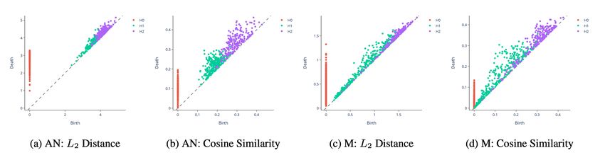
The persistence diagrams of the Euclidean embeddings under both metrics and for both datasets are given
in Figure 6. We see that up to scaling, the persistence diagrams for both embeddings into Euclidean space
with respect to the L2 metric and cosine similarity are similar in terms of location and distribution of H0 ,
H1 , and H2 points on the persistence diagrams. We quantify this similarity by computing dilation-invariant
bottleneck dissimilarities. The graphs of the search procedure for each dataset are given in Figure 8. We first
note that the standard bottleneck distances between the L2 and cosine similarity persistence diagrams are
1.642 for the ActivityNet dataset, and 0.6625 for the Mammals dataset. The dilation-invariant bottleneck
16Figure 6: Persistence Diagrams of Euclidean Embeddings. AN: ActivityNet, M: Mammals.
Figure 7: Persistence Diagrams of Poincaré Embeddings. AN: ActivityNet, M: Mammals, expmap signifies
Euclidean optimization followed by an exponential map embedding into the Poincaré ball, while Poincaré
signifies direct optimization on the Poincaré ball.
dissimilarities are achieved at the minimum value of the bottleneck distance in our parameter search region.
The dilation-invariant bottleneck dissimilarities from cosine similarity to L2 are 1.311 for the ActivityNet
dataset and 0.3799 for the Mammals dataset.
The dilation parameter for Euclidean embeddings can be alternatively searched according to the scale of
L2 embedded points as follows. Since mutual distances under the cosine embedding are always bounded by
1, we can regard the induced finite metric space as a baseline. For the L2 embedding, mutual dissimilarities
are affected by the scale of the embedded point cloud, i.e., if we multiply the points by a factor R, the
induced metric will also dilate by a factor R. In experiments, the scale is 18.13 for the L2 embedding of
ActivityNet and 3.188 for Mammals, which are consistent with dilation parameters we found.
The visual compatibility of the persistence diagrams together with the small dilation-invariant bottleneck
distances indicate that the topology of the database is preserved in the Euclidean embedding, irrespective
of the metric.
4.1.2 Topology of the Poincaré Ball Embeddings
The persistence diagrams for the Poincaré ball embeddings for both datasets are given in Figure 7. For
the ActivityNet dataset, we see that both embeddings fail to identify the H1 and H2 homology inherent
in the dataset (see Figure 5), which, by contrast, the Euclidean embeddings successfully capture. For the
Mammals dataset, only the exponential map embedding into the Poincaré ball is able to identify H1 and H2
homology, but note that these are all points close to the diagonal. Their position on the diagonal indicates
that the persistence of their corresponding topological features is not significant: these features are born and
die almost immediately, are therefore likely to be topological noise. We now investigate this phenomenon
further.
From (18), we note that an alternative representation for the distance function maybe obtained as follows.
173.25
Different Dilations 0.75 Different Dilations
7
6.10 3.00 No Dilation No Dilation
Optimal Dilation 0.70 Optimal Dilation
6
6.05 2.75
0.65
Bottleneck Distances
Bottleneck Distances
Bottleneck Distances
Bottleneck Distances
5 2.50
6.00
Different Dilations Different Dilations 0.60
4 No Dilation No Dilation 2.25
5.95
Optimal Dilation Optimal Dilation 0.55
3 2.00
5.90 0.50
2 1.75
5.85 0.45
1.50
1 0.40
5.80
1.25
0.0 0.2 0.4 0.6 0.8 1.0 1.5 2.0 2.5 3.0 5 10 15 20 25 30 35 2 3 4 5 6 7 8
Dilation Parameters Dilation Parameters Dilation Parameters Dilation Parameters
(a) AN Poincaré (b) M Poincaré (c) AN Euclidean (d) M Euclidean
Figure 8: Dilation-Invariant Bottleneck Distances Between Embeddings. AN: ActivityNet, M: Mammals
Set
2kx − yk2
A(x, y) := 1 + , (19)
(1 − kxk2 )(1 − kyk2 )
then (18) may be rewritten as
p
dP (x, y) = log(A(x, y) + A(x, y)2 − 1). (20)
We assume that kx − yk has a strictly positive lower bound and study the case when both points x, y lie
near the boundary, i.e., both kxk ≈ 1 and kyk ≈ 1. Notice, then, that (19) and (20) are approximated by
1 kx − yk2
A(x, y) ≈ ,
2 (1 − kxk)(1 − kyk)
dP (x, y) ≈ log(2A(x, y))
≈ 2log(kx − yk) − log(1 − kxk) − log(1 − kyk). (21)
Notice also that
dP (x, 0) ≈ log2 − log(1 − kxk). (22)
Combining (21) and (22) yields the following approximation for the Poincaré distance:
dP (x, y) ≈ dP (x, 0) + dP (y, 0) + 2log(kx − yk/2). (23)
For points near the boundary, i.e., dP (x, 0) = R
1, (23) gives a mutual distance of approximately 2R
between any given pair of points.
Recall from Definition 2 that a k-simplex is spanned if and only if the mutual distances between k + 1
points are less than a given threshold r. The implication for discrete points near the boundary of the
Poincaré ball is that either the threshold is less than 2R, and then the VR complex is a set of 0-simplices;
or the threshold is greater than 2R, and then the VR complex is homeomorphic to a simplex in higher
dimensions. That is, the VR filtration jumps from discrete points to a highly connected complex; this
behavior is illustrated in Figure 9.
This phenomenon of sharp phase transition is observable in our applications, which we further explore
through numerical experiments and display in Figure 10. Here, each curve corresponds to a numerical
experiment. We also plot the corresponding connectivity of VR complexes with respect to the Euclidean
distance for comparison. For a given experiment, we draw the distance cumulative distribution function as
follows: first, we normalize distances and sort them in ascending order; next, for the kth element Rk , we
compute the proportion of connected pairs as
#{(xi , xj ) | dP (xi , xj ) ≤ Rk }
. (24)
#{(xi , xj )}
From the cumulative distribution plot in Figure 10, we see this rapidly increasing connectivity behavior at
higher threshold values in repeated numerical experiments. In each experiment, points are sampled closer and
18You can also read