Transformer in Transformer
←
→
Page content transcription
If your browser does not render page correctly, please read the page content below
Transformer in Transformer

                                               Kai Han1,2 An Xiao1 Enhua Wu2 Jianyuan Guo1 Chunjing Xu1 Yunhe Wang1
                                                                    1
                                                                      Noah’s Ark Lab, Huawei Technologies
                                                            2
                                                              State Key Lab of Computer Science, ISCAS & UCAS
                                             {kai.han,an.xiao,jianyuan.guo,xuchunjing,yunhe.wang}@huawei.com, ehwu@um.edu.mo
arXiv:2103.00112v1 [cs.CV] 27 Feb 2021

                                                                                      Abstract
                                                  Transformer is a type of self-attention-based neural networks originally applied
                                                  for NLP tasks. Recently, pure transformer-based models are proposed to solve
                                                  computer vision problems. These visual transformers usually view an image as a
                                                  sequence of patches while they ignore the intrinsic structure information inside each
                                                  patch. In this paper, we propose a novel Transformer-iN-Transformer (TNT) model
                                                  for modeling both patch-level and pixel-level representation. In each TNT block,
                                                  an outer transformer block is utilized to process patch embeddings, and an inner
                                                  transformer block extracts local features from pixel embeddings. The pixel-level
                                                  feature is projected to the space of patch embedding by a linear transformation layer
                                                  and then added into the patch. By stacking the TNT blocks, we build the TNT model
                                                  for image recognition. Experiments on ImageNet benchmark and downstream
                                                  tasks demonstrate the superiority and efficiency of the proposed TNT architecture.
                                                  For example, our TNT achieves 81.3% top-1 accuracy on ImageNet which is
                                                  1.5% higher than that of DeiT with similar computational cost. The code will
                                                  be available at https://github.com/huawei-noah/noah-research/tree/
                                                  master/TNT.

                                         1    Introduction
                                         Transformer is a type of neural network mainly based on self-attention mechanism [34]. Transformer
                                         is widely used in the field of natural language processing (NLP), e.g., the famous BERT [9] and GPT-
                                         3 [4] models. Inspired by the breakthrough of transformer in NLP, researchers have recently applied
                                         transformer to computer vision (CV) tasks such as image recognition [10, 31], object detection [5, 39],
                                         and image processing [6]. For example, DETR [5] treats object detection as a direct set prediction
                                         problem and solve it using a transformer encoder-decoder architecture. IPT [6] utilizes transformer
                                         for handling multiple low-level vision tasks in a single model. Compared to the mainstream CNN
                                         models [20, 14, 30], these transformer-based models have also shown promising performance on
                                         visual tasks [11].
                                         CV models purely based on transformer are attractive because they provide an computing paradigm
                                         without the image-specific inductive bias, which is completely different from convolutional neural
                                         networks (CNNs). Chen et.al proposed iGPT [7], the pioneering work applying pure transformer
                                         model on image recognition by self-supervised pre-training. ViT [10] views an image as a sequence
                                         of patches and perform classification with a transformer encoder. DeiT [31] further explores the
                                         data-efficient training and distillation of ViT. Compared to CNNs, transformer-based models can also
                                         achieve competitive accuracy without inductive bias, e.g., DeiT trained from scratch has an 81.8%
                                         ImageNet top-1 accuracy by using 86.4M parameters and 17.6B FLOPs.
                                         In ViT [10], an image is split into a sequence of patches and each patch is simply transformed into a
                                         vector (embedding). The embeddings are processed by vanilla transformer block. By doing so, ViT
                                         can process images by a standard transformer with few modifications. This design also affects the
                                         subsequent works including DeiT [31], ViT-FRCNN [2], IPT [6] and SETR [38]. However, these

                                         Preprint. Under review.
(a) TNT framework.                                     (b) TNT block.

Figure 1: Illustration of the proposed Transformer-iN-Transformer (TNT) framework. The position
embedding is not drawn for neatness. T-Block denotes transformer block.

visual transformers ignore the local relation and structure information inside the patch which is
important for visual recognition [22, 3]. By projecting the patch into a vector, the spatial structure is
corrupted and hard to learn.
In this paper, we propose a novel Transformer-iN-Transformer (TNT) architecture for visual recogni-
tion as shown in Fig. 1. Specifically, an image is split into a sequence of patches and each patch is
reshaped to (super) pixel sequence. The patch embeddings and pixel embeddings are obtained by a
linear transformation from the patches and pixels respectively, and then they are fed into a stack of
TNT blocks for representation learning. In the TNT block, there are two transformer blocks where
the outer transformer block models the global relation among patch embeddings, and the inner one
extracts local structure information of pixel embeddings. The local information is added on the patch
embedding by linearly projecting the pixel embeddings into the space of patch embedding. Patch-level
and pixel-level position embeddings are introduced in order to retain spatial information. Finally,
the class token is used for classification via a MLP head. Through the proposed TNT model, we
can model both global and local structure information of the images and improve the representation
ability of the feature. Experiments on ImageNet benchmark and downstream tasks demonstrate
the superiority of our method in terms of accuracy and FLOPs. For example, our TNT-S achieves
81.3% ImageNet top-1 with only 5.2B FLOPs, which is 1.5% higher than that of DeiT with similar
computational cost.

2     Approach
In this section, we describe the proposed transformer-in-transformer architecture and analyze the
complexity in details.

2.1   Preliminaries

We first briefly describe the basic components in transformer [34], including MSA (Multi-head
Self-Attention), MLP (Multi-Layer Perceptron) and LN (Layer Normalization).

MSA. In the self-attention module, the inputs X ∈ Rn×d are linearly transformed to three parts,
i.e., queries Q ∈ Rn×dk , keys K ∈ Rn×dk and values V ∈ Rn×dv where n is the sequence length, d,
dk , dv are the dimensions of inputs, queries (keys) and values, respectively. The scaled dot-product
attention is applied on Q, K, V :
                                                            QK T
                              Attention(Q, K, V ) = softmax( √ )V.                                   (1)
                                                              dk
Finally, a linear layer is used to produce the output. Multi-head self-attention splits the queries, keys
and values for h times and perform the attention function in parallel, and then the output values of
each head are concatenated and linearly projected to form the final output.

                                                   2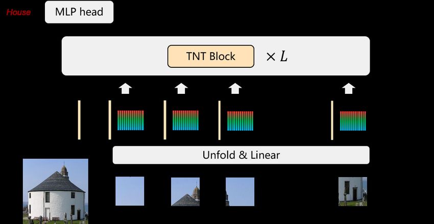
MLP. The MLP is applied between self-attention layers for feature transformation and non-linearity:

                                  MLP(X) = σ(XW1 + b1 )W2 + b2 ,                                          (2)
                d×dm                 dm ×d
where W1 ∈ R       and W2 ∈ R         are weights of the two fully-connected layers respectively,
b1 ∈ Rdm and b2 ∈ Rd are the bias terms, and σ(·) is the activation function such as GELU [15].

LN. Layer normalization [1] is a key part in transformer for stable training and faster convergence.
LN is applied over each sample x ∈ Rd as follows:
                                                           x−µ
                                            LN(x) =            ◦γ+β                                       (3)
                                                            δ
where µ ∈ R, δ ∈ R are the mean and standard deviation of the feature respectively, ◦ is the
element-wise dot, and γ ∈ Rd , β ∈ Rd are learnable affine transform parameters.

2.2   Transformer in Transformer

Given a 2D image, we uniformly split it into n patches X = [X 1 , X 2 , · · · , X n ] ∈ Rn×p×p×3 , where
(p, p) is the resolution of each image patch. ViT [10] just utilizes a standard transformer to process the
sequence of patches which corrupts the local structure of a patch, as shown in Fig. 1(a). Instead, we
propose Transformer-iN-Transformer (TNT) architecture to learn both global and local information in
an image. In TNT, each patch is further transformed into the target size (p0 , p0 ) with pixel unfold [26],
and with a linear projection, the sequence of patch tensors is formed as
                                                                             0   0
                                Y0 = [Y01 , Y02 , · · · , Y0n ] ∈ Rn×p ×p ×c ,                            (4)
                0   0
where Y0i ∈ Rp ×p ×c , i = 1, 2, · · · , n, and c is the number of channels. In particular, we view each
patch tensor Y0i as a sequence of pixel embeddings:

                                        Y0i = [y0i,1 , y0i,2 , · · · , y0i,m ]                            (5)

where m = p02 , and y0i,j ∈ Rc , j = 1, 2, · · · , m.
In TNT, we have two data flows in which one flow operates across the patch and the other processes
the pixels inside each patch. For the pixel embeddings, we utilize a transformer block to explore the
relation between pixels:
                                        i
                                     Y 0 l = Yl−1
                                               i             i
                                                  + MSA(LN(Yl−1 )),                                       (6)
                                                  0i                    0i
                                      Yli   =Y     l   + MLP(LN(Y        l )).                            (7)
where l = 1, 2, · · · , L is index of the l-th layer, and L is the total number of layers. All patch tensors
after transformation are Yl = [Yl1 , Yl2 , · · · , Yln ]. This can be viewed as an inner transformer block,
denoted as Tin . This process builds the relationship among pixels by computing interactions between
any two pixels. For example, in a patch of human face, a pixel belonging to the eye is more related to
other pixels of eyes while interacts less with forehead pixels.
For the patch level, we create the patch embedding memories to store the sequence of patch-level
representations: Z0 = [Zclass , Z01 , Z02 , · · · , Z0n ] ∈ R(n+1)×d where Zclass is the classification token
similar to ViT [10], and all of them are initialized as zero. In each layer, the patch tensors are
transformed into the domain of patch embeddings by linear projection and added into the patch
embeddings:
                                 i            i              i
                              Zl−1    = Zl−1        + Vec(Yl−1  )Wl−1 + bl−1 ,                             (8)
        i
where Zl−1 ∈ Rd , Vec(·) flattens the input to a vector, and Wl−1 ∈ Rmc×d and bl−1 ∈ Rd are the
weights and bias respectively. We use the standard transformer block for transforming the patch
embeddings:
                                       i
                                    Z 0 l = Zl−1
                                             i             i
                                                 + MSA(LN(Zl−1 )),                                        (9)
                                                   i                  i
                                     Zli    =   Z 0l   +   MLP(LN(Z 0 l )).                              (10)
This outer transformer block Tout is used for modeling relationship among patch embeddings.

                                                             3
In summary, the inputs and outputs of the TNT block include the pixel embeddings and patch
embeddings as shown in Fig. 1(b), so the TNT can be formulated as
Yl , Zl = TNT(Yl−1 , Zl−1 ). (11)
In our TNT block, the inner transformer block is used to model the relationship between pixels for
local feature extraction, and the outer transformer block captures the intrinsic information from the
sequence of patches. By stacking the TNT blocks for L times, we build the transformer-in-transformer
network. Finally, the classification token serves as the image representation and a fully-connected
layer is applied for classification.
Position encoding. Spatial information is an
important factor in image recognition. For patch
embeddings and pixels embeddings, we both
add the corresponding position encodings to re-
tain spatial information as shown in Fig. 2. The
standard learnable 1D position encodings are uti-
lized here. Specifically, each patch is assigned
with a position encodings:
Z0 ← Z0 + Epatch , (12)
where Epatch ∈ R(n+1)×d are the patch posi-
tion encodings. As for the pixels in a patch, a
Figure 2: Patch-level and pixel-level position en-
pixel position encoding is added to each pixel
codings.
embedding:
Y0i ← Y0i + Epixel , i = 1, 2, · · · , n (13)
where Epixel ∈ Rm×c are the pixel position encodings which are shared across patches. In this way,
patch position encoding can maintain the global spatial information, while pixel position encoding is
used for preserving the local relative position.
2.3 Complexity Analysis
A standard transformer block includes two parts, i.e., the multi-head self-attention and multi-layer
perceptron. The FLOPs of MSA are 2nd(dk + dv ) + n2 (dk + dv ), and the FLOPs of MLP are
2ndv rdv where r is the dimension expansion ratio of hidden layer in MLP. Overall, the FLOPs of a
standard transformer block are
FLOPsT = 2nd(dk + dv ) + n2 (dk + dv ) + 2nddr. (14)
Since r is usually set as 4, and the dimensions of input, key (query) and value are usually set as the
same, the FLOPs calculation can be simplified as
FLOPsT = 2nd(6d + n). (15)
The number of parameters can be obtained as
ParamsT = 12dd. (16)
Our TNT block consists of three parts: an inner transformer block Tin , an outer transformer block
Tout and a linear layer. The computation complexity of Tin and Tout are 2nmc(6c + m) and
2nd(6d + n) respectively. The linear layer has FLOPs of nmcd. In total, the FLOPs of TNT block
are
FLOPsT N T = 2nmc(6c + m) + nmcd + 2nd(6d + n). (17)
Similarly, the parameter complexity of TNT block is calculated as
ParamsT N T = 12cc + mcd + 12dd. (18)
Although we add two more components in our TNT block, the increase of FLOPs is small since
c
d and O(m) ≈ O(n) in practice. For example, in the ViT-B/16 configuration, we have d = 768
and n = 196. We set c = 12 and m = 64 in our structure of TNT-B correspondingly. From Eq. 15
and Eq. 17, we can obtain that FLOPsT = 1446M and FLOPsT N T = 1603M . The FLOPs ratio of
TNT block over standard transformer block is about 1.09×. Similarly, the parameters ratio is about
1.08×. With a small increase of computation and memory cost, our TNT block can efficiently model
the local structure information and achieve a much better trade-off between accuracy and complexity
as demonstrated in the experiments.
42.4 Network Architecture
We build our TNT architectures by following the basic configuration of ViT [10] and DeiT [31].
The patch size is set as 16×16. The unfolded patch size p0 is set as 4 by default, and other size
values are evaluated in the ablation studies. As shown in Table 1, there are two variants of TNT
networks with different model size, namely, TNT-S and TNT-B. They consist of 23.8M and 65.6M
parameters respectively. The corresponding FLOPs for processing a 224×224 image are 5.2B and
14.1B respectively.
Operational optimizations. Inspired by squeeze-and-excitation (SE) network for CNNs [17], we
propose to explore channel-wise attention for transformers. We first average all the patch (pixel)
embeddings and use a two-layer MLP to calculate the attention values. The attention is multiplied
to all the embeddings. The SE module only brings in a few extra parameters but is able to perform
dimension-wise attention for feature enhancement.
Table 1: Variants of our TNT architecture. ‘S’ means small, ‘B’ means base. The FLOPs are
calculated for images at resolution 224×224.
Inner transformer Outer transformer Params FLOPs
Model Depth
dim c #heads MLP r dim d #heads MLP r (M) (B)
TNT-S (ours) 12 24 4 4 384 6 4 23.8 5.2
TNT-B (ours) 12 40 4 4 640 10 4 65.6 14.1
3 Experiments
In this section, we conduct extensive experiments on visual benchmarks to evaluate the effectiveness
of the proposed TNT architecture.
3.1 Datasets and Experimental Settings
Datasets. ImageNet ILSVRC 2012 [28] is an image classification benchmark consisting of 1.2M
training images belonging to 1000 classes, and 50K validation images with 50 images per class. We
adopt the same data augmentation strategy as that in DeiT [31] including random crop, random clip,
Rand-Augment [8], Mixup [37] and CutMix [36].
In addition to ImageNet, we also test on the downstream tasks with transfer learning to evaluate the
generalization of TNT. The details of used visual datasets are listed in Table 2. The data augmentation
strategy are the same as that of ImageNet.
Table 2: Details of used visual datasets.
Dataset Train size Test size #Classes
ImageNet [28] 1,281,167 50,000 1000
Fine-grained
Oxford 102 Flowers [24] 2,040 6,149 102
Oxford-IIIT Pets [25] 3,680 3,669 37
Superordinate-level
CIFAR-10 [18] 50,000 10,000 10
CIFAR-100 [18] 50,000 10,000 100
Implementation Details. We utilize the training strategy provided in DeiT [31]. The main ad-
vanced technologies apart from common setting [14] include AdamW [21], label smoothing [29],
DropPath [19], repeated augmentation [16]. We list the hyper-parameters in Table 3 for better
understanding. All the models are implemented using PyTorch [26] and trained on NVIDIA Tesla
V100 GPUs.
5Table 3: Default training hyper-parameters used in our method, unless stated otherwise.
Batch Learning LR Weight Warmup Label Drop Repeated
Epochs Optimizer
size rate decay decay epochs smooth path Aug
√
300 AdamW 1024 1e-3 cosine 0.05 5 0.1 0.1
3.2 TNT on ImageNet
We train our TNT models with the same training setting as that of DeiT [31]. The recent transformer-
based models like ViT [10] and DeiT [31] are compared. To have a better understanding of current
progress of visual transformers, we also include the representative CNN-based models such as
ResNet [14], RegNet [27] and EfficientNet [30]. The results are shown in Table 4. We can see that
our transformer-based model, i.e., TNT outperforms all the other visual transformer models. In
particular, TNT-S achieves 81.3% top-1 accuracy which is 1.5% higher than the baseline model DeiT-
S, indicating the benefit of the introduced TNT framework to preserve local structure information
inside the patch. By adding SE module, TNT-S model can be further improved to obtain 81.6%
top-1. Compared to CNNs, TNT can outperform the widely-used ResNet and RegNet. Note that
all the transformer-based models are still inferior to EfficientNet which utilizes special depth-wise
convolutions, so it is yet a challenge of how to beat EfficientNet using pure transformer.
Table 4: Results of TNT and other networks on ImageNet.
Model Resolution Params (M) FLOPs (B) Top-1 (%) Top-5 (%)
CNN-based
ResNet-50 [14] 224×224 25.6 4.1 76.2 92.9
ResNet-152 [14] 224×224 60.2 11.5 78.3 94.1
RegNetY-8GF [27] 224×224 39.2 8.0 79.9 -
RegNetY-16GF [27] 224×224 83.6 15.9 80.4 -
GhostNet-A [12, 13] 240×240 11.9 0.6 79.4 94.5
EfficientNet-B3 [30] 300×300 12.0 1.8 81.6 94.9
EfficientNet-B4 [30] 380×380 19.0 4.2 82.9 96.4
Transformer-based
DeiT-S [31] 224×224 22.1 4.6 79.8 -
T2T-ViT_t-14 [35] 224×224 21.5 5.2 80.7 -
TNT-S (ours) 224×224 23.8 5.2 81.3 95.6
TNT-S + SE (ours) 224×224 24.7 5.2 81.6 95.7
ViT-B/16 [10] 384×384 86.4 55.5 77.9 -
DeiT-B [31] 224×224 86.4 17.6 81.8 -
TNT-B (ours) 224×224 65.6 14.1 82.8 96.3
We also plot the accuracy-parameters and accuracy-FLOPs line charts in Fig. 3 to have an intuitive
comparison of these models. Our TNT models consistently outperform other transformer-based
models by a significant margin.
Table 5: Effect of position encoding.
Model Patch position encoding Pixel position encoding Top-1 (%)
% % 80.5
TNT-S " % 80.8
% " 80.7
" " 81.3
3.3 Ablation Studies
Effect of position encodings. Position information is important for image recognition. In TNT
structure, patch position encoding is for maintaining global spatial information, and pixel position
encoding is used to preserve local relative position. We verify their effect by removing them separately.
As shown in Table 5, we can see that TNT-S with both patch position encoding and pixel position
683 83
82 82
81 81
80 80
Accuracy (%)
Accuracy (%)
79 79
78 78
77 77
TNT ResNet TNT ResNet
76 ViT ResNeXt 76 ViT ResNeXt
DeiT RegNet DeiT RegNet
75 75
20 30 40 50 60 70 80 90 4 6 8 10 12 14 16 18 20
Params (M) FLOPs (B)
(a) Acc v.s. Params (b) Acc v.s. FLOPs
Figure 3: Performance comparison of the representative visual backbone networks on ImageNet.
encoding performs the best by achieving 81.3% top-1 accuracy. Removing patch/pixel position
encoding brings in a 0.6%/0.5% accuracy drop respectively, and removing all position encodings
heavily decrease the accuracy by 0.8%.
Number of #heads. The effect of #heads in standard transformer has been investigated in multiple
works [23, 34] and a head width of 64 is recommended for visual tasks [10, 31]. We adopt the head
width of 64 in outer transformer block in our model. The number of heads in inner transformer block
is another hyper-parameter for investigation. We evaluate the effect of #heads in inner transformer
block (Table 6). We can see that a proper number of heads (e.g., 2 or 4) achieve the best performance.
Table 6: Effect of #heads in inner transformer block in TNT-S.
#heads 1 2 4 8
Top-1 81.0 81.3 81.3 81.1
Transformed patch size (p0 , p0 ). In TNT, the input im- Table 7: Effect of p0 .
age is split into a number of 16×16 patches and each patch p 0
Params FLOPs Top-1
is further transformed into size (p0 , p0 ) for computational
efficiency. Here we test the effect of hyper-parameter p0 2 23.8M 5.1B 81.0%
on TNT-S architecture. As shown in Table 7, we can see 4 23.8M 5.2B 81.3%
0 8 25.1M 6.0B 81.1%
that the value of p has slight influence on the performance,
0
and we use p = 4 by default for its efficiency, unless stated otherwise.
TNT
DeiT
(a) Feature maps in Block-1/6/12. (b) T-SNE of Block-12.
Figure 4: Visualization of the features of DeiT-S and TNT-S.
73.4 Visualization
We visualize the learned features of DeiT and TNT to further understand the effect of the proposed
method. For better visualization, the input image is resized to 1024×1024. The feature maps are
formed by reshaping the patch embeddings according to their spatial positions. The feature maps in
the 1-st, 6-th and 12-th blocks are shown in Fig. 4(a) where 12 feature maps are randomly sampled
for these blocks each. In TNT, the local information are better preserved compared to DeiT. We also
visualize all the 384 feature maps in the 12-th block using t-SNE [33] (Fig. 4(b)). We can see that the
features of TNT are more diverse and contain richer information than those of DeiT. These benefits
owe to the introduction of inner transformer block for modeling local features.
In addition to the patch-level features, we also visualize the pixel embeddings of TNT in Fig. 5. For
each patch, we reshape the pixel embeddings according to their spatial positions to form the feature
maps and then average these feature maps by the channel dimension. The averaged feature maps
corresponding to the 14×14 patches are shown in Fig. 5. We can see that the local information is
well preserved in the shallow layers, and the representations become more abstract gradually as the
network goes deeper.
Figure 5: Visualization of the averaged pixel embeddings of TNT-S.
3.5 Transfer Learning
To demonstrate the strong generalization ability of TNT, we tranfer TNT-S, TNT-B models trained
on ImageNet to other benchmark datasets. More specifically, we evaluate our models on 4 image
classification datasets with traning set size ranging from 2,040 to 50,000 images. These datasets
include superordinate-level object classification (CIFAR-10 [18], CIFAR-100 [18]) and fine-grained
object classification (Oxford-IIIT Pets [25], Oxford 102 Flowers [24]), shown in Table 2. All models
are fine-tuned with an image resolution of 384×384. Table 8 compares the transfer learing results of
TNT to those of VIT, DeiT and other convlutional networks. We find that TNT outperforms DeiT in
most datasets with less parameters, which shows the supreority of modeling pixel-level relations to
get better feature resprentation.
Fine-tuning Details. We adopt the same training settings as those at the pre-training stage by
perserving all data augmentation strategies. In order to fine-tune in a different resolution, we also
interpolate the position embeddings of new patches. For CIFAR-10 and CIFAR-100, we fine-tune the
models for 64 epochs, and for fine-grained datasets, we fine-tune the models for 300 epochs.
Table 8: Results on downstream tasks with ImageNet pre-training. ↑ 384 denotes fine-tuning with
384×384 resolution.
Model Params (M) ImageNet CIFAR10 CIFAR100 Flowers Pets
CNN-based
Grafit ResNet-50 [32] 25.6 79.6 - - 98.2 -
Grafit RegNetY-8GF [32] 39.2 - - - 99.1 -
EfficientNet-B5 [30] 30 83.6 98.7 91.1 98.5 -
Transformer-based
ViT-B/16↑384 86.4 77.9 98.1 87.1 89.5 93.8
DeiT-B↑384 86.4 83.1 99.1 90.8 98.4 -
TNT-S↑384 (ours) 23.8 83.1 98.7 90.1 98.8 94.7
TNT-B↑384 (ours) 65.6 83.9 99.1 91.1 99.0 95.0
84 Conclusion
In this paper, we propose a novel Transformer-iN-Transformer (TNT) network architecture for visual
recognition. In particular, we uniformly split the image into a sequence of patches and view each
patch as a sequence of pixels. We introduce a TNT block in which an outer transformer block
is utilized for processing the patch embeddings and an inner transformer block is used to model
the relation among pixel embeddings. The information of pixel embeddings is added on the patch
embedding after the projection of a linear layer. We build our TNT architecture by stacking the TNT
blocks. Compared to the conventional vision transformers (ViT) which corrupts the local structure
of the patch, our TNT can better preserve and model the local information for visual recognition.
Extensive experiments on ImageNet and downstream tasks have demonstrate the effectiveness of the
proposed TNT architecture.
References
[1] Jimmy Lei Ba, Jamie Ryan Kiros, and Geoffrey E Hinton. Layer normalization. arXiv preprint
arXiv:1607.06450, 2016.
[2] Josh Beal, Eric Kim, Eric Tzeng, Dong Huk Park, Andrew Zhai, and Dmitry Kislyuk. Toward
transformer-based object detection. arXiv preprint arXiv:2012.09958, 2020.
[3] Wieland Brendel and Matthias Bethge. Approximating CNNs with bag-of-local-features models
works surprisingly well on imagenet. In ICLR, 2019.
[4] Tom B Brown, Benjamin Mann, Nick Ryder, Melanie Subbiah, Jared Kaplan, Prafulla Dhariwal,
Arvind Neelakantan, Pranav Shyam, Girish Sastry, Amanda Askell, et al. Language models are
few-shot learners. In NeurIPS, 2020.
[5] Nicolas Carion, Francisco Massa, Gabriel Synnaeve, Nicolas Usunier, Alexander Kirillov, and
Sergey Zagoruyko. End-to-end object detection with transformers. In ECCV, 2020.
[6] Hanting Chen, Yunhe Wang, Tianyu Guo, Chang Xu, Yiping Deng, Zhenhua Liu, Siwei Ma,
Chunjing Xu, Chao Xu, and Wen Gao. Pre-trained image processing transformer. arXiv preprint
arXiv:2012.00364, 2020.
[7] Mark Chen, Alec Radford, Rewon Child, Jeffrey Wu, Heewoo Jun, David Luan, and Ilya
Sutskever. Generative pretraining from pixels. In ICML, 2020.
[8] Ekin D Cubuk, Barret Zoph, Jonathon Shlens, and Quoc V Le. Randaugment: Practical
automated data augmentation with a reduced search space. In CVPR Workshops, 2020.
[9] Jacob Devlin, Ming-Wei Chang, Kenton Lee, and Kristina Toutanova. Bert: Pre-training of
deep bidirectional transformers for language understanding. In NAACL-HLT (1), 2019.
[10] Alexey Dosovitskiy, Lucas Beyer, Alexander Kolesnikov, Dirk Weissenborn, Xiaohua Zhai,
Thomas Unterthiner, Mostafa Dehghani, Matthias Minderer, Georg Heigold, Sylvain Gelly, et al.
An image is worth 16x16 words: Transformers for image recognition at scale. arXiv preprint
arXiv:2010.11929, 2020.
[11] Kai Han, Yunhe Wang, Hanting Chen, Xinghao Chen, Jianyuan Guo, Zhenhua Liu, Yehui
Tang, An Xiao, Chunjing Xu, Yixing Xu, et al. A survey on visual transformer. arXiv preprint
arXiv:2012.12556, 2020.
[12] Kai Han, Yunhe Wang, Qi Tian, Jianyuan Guo, Chunjing Xu, and Chang Xu. Ghostnet: More
features from cheap operations. In CVPR, 2020.
[13] Kai Han, Yunhe Wang, Qiulin Zhang, Wei Zhang, Chunjing Xu, and Tong Zhang. Model rubik’s
cube: Twisting resolution, depth and width for tinynets. NeurIPS, 2020.
[14] Kaiming He, Xiangyu Zhang, Shaoqing Ren, and Jian Sun. Deep residual learning for image
recognition. In CVPR, 2016.
[15] Dan Hendrycks and Kevin Gimpel. Gaussian error linear units (gelus). arXiv preprint
arXiv:1606.08415, 2016.
[16] Elad Hoffer, Tal Ben-Nun, Itay Hubara, Niv Giladi, Torsten Hoefler, and Daniel Soudry.
Augment your batch: Improving generalization through instance repetition. In CVPR, 2020.
[17] Jie Hu, Li Shen, and Gang Sun. Squeeze-and-excitation networks. In CVPR, 2018.
9[18] Alex Krizhevsky, Geoffrey Hinton, et al. Learning multiple layers of features from tiny images.
2009.
[19] Gustav Larsson, Michael Maire, and Gregory Shakhnarovich. Fractalnet: Ultra-deep neural
networks without residuals. arXiv preprint arXiv:1605.07648, 2016.
[20] Min Lin, Qiang Chen, and Shuicheng Yan. Network in network. In ICLR, 2014.
[21] Ilya Loshchilov and Frank Hutter. Decoupled weight decay regularization. arXiv preprint
arXiv:1711.05101, 2017.
[22] David G Lowe. Object recognition from local scale-invariant features. In ICCV, 1999.
[23] Paul Michel, Omer Levy, and Graham Neubig. Are sixteen heads really better than one? In
NeurIPS, 2019.
[24] Maria-Elena Nilsback and Andrew Zisserman. Automated flower classification over a large
number of classes. In 2008 Sixth Indian Conference on Computer Vision, Graphics & Image
Processing, pages 722–729. IEEE, 2008.
[25] Omkar M Parkhi, Andrea Vedaldi, Andrew Zisserman, and CV Jawahar. Cats and dogs. In 2012
IEEE conference on computer vision and pattern recognition, pages 3498–3505. IEEE, 2012.
[26] Adam Paszke, Sam Gross, Francisco Massa, Adam Lerer, James Bradbury, Gregory Chanan,
Trevor Killeen, Zeming Lin, Natalia Gimelshein, Luca Antiga, et al. Pytorch: An imperative
style, high-performance deep learning library. NeurIPS, 2019.
[27] Ilija Radosavovic, Raj Prateek Kosaraju, Ross Girshick, Kaiming He, and Piotr Dollár. Design-
ing network design spaces. In CVPR, 2020.
[28] Olga Russakovsky, Jia Deng, Hao Su, Jonathan Krause, Sanjeev Satheesh, Sean Ma, Zhiheng
Huang, Andrej Karpathy, Aditya Khosla, Michael Bernstein, et al. Imagenet large scale visual
recognition challenge. International Journal of Computer Vision, 115(3):211–252, 2015.
[29] Christian Szegedy, Vincent Vanhoucke, Sergey Ioffe, Jon Shlens, and Zbigniew Wojna. Re-
thinking the inception architecture for computer vision. In CVPR, 2016.
[30] Mingxing Tan and Quoc Le. Efficientnet: Rethinking model scaling for convolutional neural
networks. In ICML, 2019.
[31] Hugo Touvron, Matthieu Cord, Matthijs Douze, Francisco Massa, Alexandre Sablayrolles, and
Hervé Jégou. Training data-efficient image transformers & distillation through attention. arXiv
preprint arXiv:2012.12877, 2020.
[32] Hugo Touvron, Alexandre Sablayrolles, Matthijs Douze, Matthieu Cord, and Hervé Jégou.
Grafit: Learning fine-grained image representations with coarse labels. arXiv preprint
arXiv:2011.12982, 2020.
[33] Laurens Van der Maaten and Geoffrey Hinton. Visualizing data using t-sne. Journal of machine
learning research, 9(11), 2008.
[34] Ashish Vaswani, Noam Shazeer, Niki Parmar, Jakob Uszkoreit, Llion Jones, Aidan N Gomez,
Łukasz Kaiser, and Illia Polosukhin. Attention is all you need. NeurIPS, 2017.
[35] Li Yuan, Yunpeng Chen, Tao Wang, Weihao Yu, Yujun Shi, Francis EH Tay, Jiashi Feng, and
Shuicheng Yan. Tokens-to-token vit: Training vision transformers from scratch on imagenet.
arXiv preprint arXiv:2101.11986, 2021.
[36] Sangdoo Yun, Dongyoon Han, Seong Joon Oh, Sanghyuk Chun, Junsuk Choe, and Youngjoon
Yoo. Cutmix: Regularization strategy to train strong classifiers with localizable features. In
ICCV, 2019.
[37] Hongyi Zhang, Moustapha Cisse, Yann N Dauphin, and David Lopez-Paz. mixup: Beyond
empirical risk minimization. arXiv preprint arXiv:1710.09412, 2017.
[38] Sixiao Zheng, Jiachen Lu, Hengshuang Zhao, Xiatian Zhu, Zekun Luo, Yabiao Wang, Yanwei
Fu, Jianfeng Feng, Tao Xiang, Philip HS Torr, et al. Rethinking semantic segmentation from a
sequence-to-sequence perspective with transformers. arXiv preprint arXiv:2012.15840, 2020.
[39] Xizhou Zhu, Weijie Su, Lewei Lu, Bin Li, Xiaogang Wang, and Jifeng Dai. Deformable detr:
Deformable transformers for end-to-end object detection. arXiv preprint arXiv:2010.04159,
2020.
10You can also read