Pose Measurement of Flexible Medical Instruments using Fiber Bragg Gratings in Multi-Core Fiber
←
→
Page content transcription
If your browser does not render page correctly, please read the page content below
This article has been accepted for publication in a future issue of this journal, but has not been fully edited. Content may change prior to final publication. Citation information: DOI 10.1109/JSEN.2020.2993452, IEEE Sensors
                                                                                                                  Journal
                                                                                                                                                                                                                 1

               Pose Measurement of Flexible Medical Instruments
                using Fiber Bragg Gratings in Multi-Core Fiber
                        Fouzia Khan, Abdulhamit Donder, Stefano Galvan, Ferdinando Rodriguez y Baena and Sarthak Misra

                 Abstract—Accurate navigation of flexible medical instruments
              like catheters require the knowledge of its pose, that is its position
              and orientation. In this paper multi-core fibers inscribed with
              fiber Bragg gratings (FBG) are utilized as sensors to measure
              the pose of a multi-segment catheter. A reconstruction technique
              that provides the pose of such a fiber is presented. First, the
              measurement from the Bragg gratings are converted to strain
              then the curvature is deduced based on those strain calculations.
              Next, the curvature and the Bishop frame equations are used
              to reconstruct the fiber. This technique is validated through
              experiments where the mean error in position and orientation is
              observed to be less than 4.69 mm and 6.48 degrees, respectively.
              The main contributions of the paper are the use of Bishop frames
              in the reconstruction and the experimental validation of the
              acquired pose.
                Index Terms—Fiber Bragg grating, bio-medical, robotics,
              shape sensing, medical instrument, 3D reconstruction, multi-core
              optical fiber, Bishop frames, Parallel transport

                                                                                                                  Fig. 1: Top: A flexible instrument model placed in a vascular
                                               I. I NTRODUCTION                                                   phantom. Bottom: Ideal reconstruction of the instrument along
                                                                                                                  the arc length s with position given as a curve, γ(s), and the
                 Flexible medical instruments are frequently used for proce-
                                                                                                                  orientation as a frame {M1 (s), M2 (s), T(s)}.
              dures in cardiology and urology. Accurate navigation of these
              instruments require spatial information such as the pose, as
              shown in Figure 1. Conventionally, fluoroscopy or ultrasound                                        acquiring the instrument tip position from endoscopic images;
              are used to monitor these instruments, even though both                                             they require an unobstructed view of the surgical site. Thus,
              methods have their drawbacks [1]. Fluoroscopy exposes the                                           they are difficult to use in practice and are applicable only to
              patient to contrast agents and to radiation. In addition, the                                       procedures that use endoscopes. An alternative technology that
              workflow of the procedure is disrupted to allow the medical                                         mitigates the requirement of unobstructed view is electromag-
              personnel time to retreat during imaging. On the other hand,                                        netic (EM) tracking. However, it has a limited workspace and
              ultrasound images have low resolution and the instruments can                                       the tracking accuracy degrades significantly in the presence of
              cause artifacts [2]. Thus, there is a need to develop imaging                                       electronic and metallic instruments [5]. Thus, EM tracking is
              and other sensing techniques to acquire the spatial information                                     better suited for controlled environments than clinical settings.
              of flexible instruments.                                                                               Another approach for acquiring spatial information is using
                 In the literature there are studies that used endoscopic im-                                     optical fibers. This is an attractive approach due to the com-
              ages for retrieving spatial information of flexible instruments.                                    patibility of the sensors with the medical environment. Optical
              Relink et al. used markers on an instrument and a state estima-                                     fibers are biocompatible, nontoxic, immune to electromagnetic
              tor to acquire the position of the instrument [3]. Cabaras et al.                                   interference and sterilizable [6]. In addition, they are small and
              used feature detection along with learning methods to detect                                        highly flexible, and thus can be easily integrated into medical
              the pose of a flexible instrument from monocular endoscopic                                         instruments [1] [7]. Sareh et al. have used the bend sensitivity
              images [4]. Although these studies show the feasibility of                                          of optical fibers to get the pose of the instrument tip [8].
                                                                                                                  This approach leads to low-cost sensing hardware, but multiple
                 This project has received funding from the European Union’s Horizon                              fibers are required that must be routed in a specific manner
              2020 Research and Innovation Programme under Grant Agreement #688279
              (EDEN2020). Abdulhamit Donder is funded by the Republic of Turkey. F.                               and it has a complex calibration procedure. The required
              Khan and S. Misra are affiliated with Surgical Robotics Laboratory, Depart-                         routing renders it inapplicable to instruments like catheters
              ment of Biomedical Engineering, University of Groningen and University of                           and needles. These issues can be mitigated by employing fiber
              Medical Center Groningen, 9713 GZ, The Netherlands. They are also affiliated
              with Department of Biomechanical Engineering, Engineering Technology,                               Bragg grating (FBG) sensors in the optical fibers.
              University of Twente, 7522 NB, The Netherlands. A. Donder, S. Galvan and                               Moore et al. calculated the shape of a multi-core fiber
              F. Rodriguez y Baena are with the Mechatronics in Medicine Laboratory,
              Department of Mechanical Engineering, Imperial College London, London                               with FBG sensors using Frenet-Serret equations [9]. Numerous
              SW7 2AZ, United Kingdom.                                                                            other studies have used FBG sensors for sensing shape of

     1558-1748 (c) 2020 IEEE. Personal use is permitted, but republication/redistribution requires IEEE permission. See http://www.ieee.org/publications_standards/publications/rights/index.html for more information.
                       Authorized licensed use limited to: UNIVERSITY OF TWENTE.. Downloaded on May 11,2020 at 06:54:20 UTC from IEEE Xplore. Restrictions apply.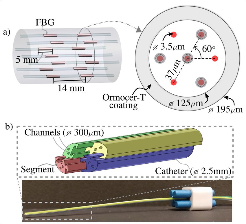
This article has been accepted for publication in a future issue of this journal, but has not been fully edited. Content may change prior to final publication. Citation information: DOI 10.1109/JSEN.2020.2993452, IEEE Sensors
                                                                                                                  Journal
                                                                                                                                                                                                                 2

              flexible instruments such as colonoscope, needle and catheter.
              Xinhua et al. acquired the shape of a colonoscope from optical
              fibers with FBG sensors in order to reduce the probability of
              loop formation during colonoscopy [10]. Park et al. placed
              optical fibers with two sets of FBG sensors on a needle to
              provide tip deflection, bend profile and temperature compen-
              sation [11]. Roesthuis et al. acquired the 3D shape of a needle
              using four sets of FBG sensors in optical fibers [12]. Khan
              et al. reconstructed the shape of a multi-segment catheter in
              3D space using multi-core fibers with six sets of FBGs in
              each fiber [13]. Lastly, Henken et al. calculated the needle tip
              deflection based on strains derived from measurements from
              two sets of FBG sensors [14]. Nevertheless, these studies have
              focused on acquiring only the position of the instrument.
                 The study presented in this paper extends the use of FBG
              sensors for acquiring the orientation of an instrument in
              addition to its position. This information can be utilized for
              improving the navigation accuracy of flexible medical instru-
              ments. The sensors are written in multi-core fibers instead of
              being written on several single-core fibers due to the space
              restriction in these instruments. The contributions of this study
              include the use of Bishop frames in the reconstruction and
              validation of the acquired pose. The reconstruction technique
              is described in Section II, followed by the experiments, dis-
              cussion and conclusion in Section III, IV and V, respectively.

                                                    II. T HEORY
                                                                                                                  Fig. 2: 1) A segment of the multi-core fiber in its initial
                 This section outlines the technique for reconstructing a
                                                                                                                  configuration. The four cores of the fiber are labeled a, b, c and
              multi-core fiber with FBG sensors. The fiber is modeled
                                                                                                                  d. Three sets of fiber Bragg gratings (FBG) sensors and their
              as a regular unit-speed space curve that is reconstructed in
                                                                                                                  local frames for curvature vector calculation are shown. 2) The
              Euclidean space using curvature vectors and Bishop frame
                                                                                                                  segment of the multi-core fiber in a bent configuration. 3) The
              equations [15] [16]. The curvature vectors of the fiber are
                                                                                                                  fiber cross section at the second set of FBG sensors when the
              calculated at every FBG sensor set using strains that are
                                                                                                                  fiber is bent. The variables required for the curvature vector
              derived from the wavelength measurements of the sensors in
                                                                                                                  calculation are illustrated; yi ∈ R>0 (where i ∈ a, b, c, d) is
              the set. Description of FBG sensor and the derivation of strain
                                                                                                                  the perpendicular distance from the FBG sensor on core i to
              values is given in Section II-A, followed by an explanation of
                                                                                                                  the neutral bending axis; ri ∈ R>0 is the radial distance from
              the curvature vector calculation in Section II-B. Lastly, the
                                                                                                                  the center to core i; θi ∈ (−π, π] is the angle from ri to the
              reconstruction using Bishop frame equations is presented in
                                                                                                                  curvature vector; θba is the angle between rb and ra and θca
              Section II-C.
                                                                                                                  is the angle between rc and ra .

              A. Fiber Bragg Grating for Strain Measurement
                 An FBG reflects back a narrow band of wavelengths from
              the optical input and transmits the rest. The reflection is due                                     0 and T0 are the initial values of the Bragg wavelength, strain
              to the grating being a periodic variation in the refractive                                         and temperature, respectively.
              index of the fiber over a short segment. The properties of the
                                                                                                                     In this study, the initial Bragg wavelength λB0 is collected
              grating are altered by strain and temperature; as a result the
                                                                                                                  when the fiber is straight so that the fiber is strain-free and
              reflected wavelength band shifts when a change in strain or
                                                                                                                  0 can be assumed to be zero. In addition, an FBG sensor is
              change in temperature is experienced by the grating [17]. The
                                                                                                                  placed in the central core of the fiber so that the strain on the
              wavelength which has the highest reflection is called the Bragg
                                                                                                                  sensor is zero when the fiber is bent and the term Σ(T − T0 )
              wavelength, λB ∈ R>0 . It is related to strain and temperature
                                                                                                                  can be acquired from it. The value of λB is measured and S
              on the grating according to the following equation [18]:
                                                                                                                  is a known constant. Thus, the strain on an FBG sensor can
                                        λB                                                                        be calculated.
                                   ln       = S( − 0 ) + Σ(T − T0 ),                                   (1)
                                        λB0                                                                         The next section presents the details on acquiring the
              where, S ∈ R is the gauge factor; Σ ∈ R is the temperature                                          curvature vectors of the fiber given the arrangement of the
              sensitivity;  ∈ R is the strain and T ∈ R is temperature. λB0 ,                                    FBG sensors within the fiber and their strain values.

     1558-1748 (c) 2020 IEEE. Personal use is permitted, but republication/redistribution requires IEEE permission. See http://www.ieee.org/publications_standards/publications/rights/index.html for more information.
                       Authorized licensed use limited to: UNIVERSITY OF TWENTE.. Downloaded on May 11,2020 at 06:54:20 UTC from IEEE Xplore. Restrictions apply.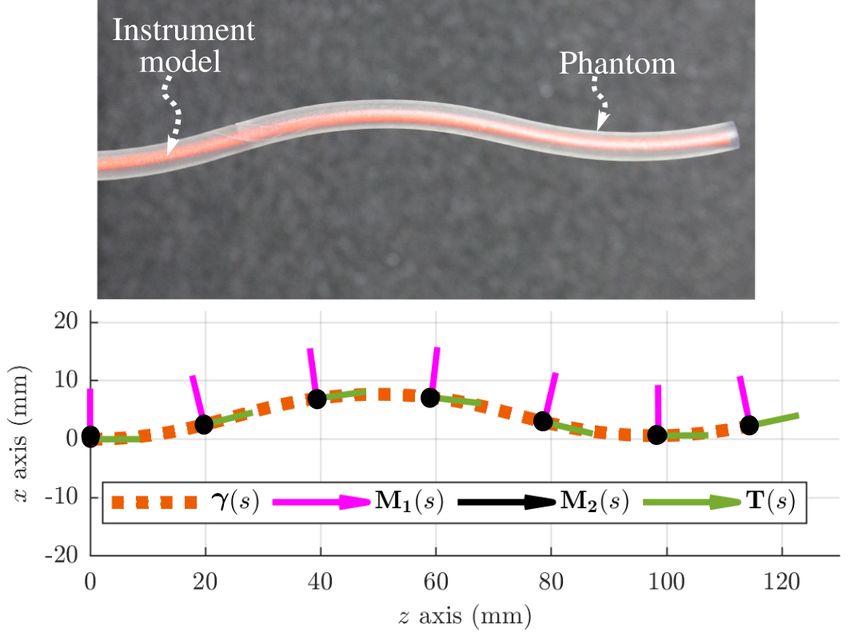
This article has been accepted for publication in a future issue of this journal, but has not been fully edited. Content may change prior to final publication. Citation information: DOI 10.1109/JSEN.2020.2993452, IEEE Sensors
Journal
3
B. Curvature Vector
The curve representing the fiber can be reconstructed if the
curvature vectors are known for the complete length of the
curve. In this study, the curvature vectors are acquired from
sets of FBG sensors placed along the length of the multi-core
fiber. Each set of FBG sensors contains four co-located FBGs,
one in the center core and three in the outer cores as shown
in Figure 2. An orthogonal frame is attached to each FBG
set such that the x and y axis are on the fiber cross section
and the x axis is from the center of the fiber to one of the
outer core, see Figure 2. The curvature vector for a set is
calculated with respect to the allocated orthogonal frame by
utilizing the relation between curvature and strain provided by
the theory of bending mechanics [19]. The strain experienced
by the FBG sensors on the outer cores is proportional to their Fig. 3: Spectra from the four cores labeled a, b, c, and d of
perpendicular distance from the neutral bending axis. Adapting a fiber as provided by the software of the interrogator FBG-
the sign convention for the strain to be positive for tension scan 804D (FBGS International NV (Geel, Belgium)). The
and negative for compression, the relation between strain and raw values in the y-axis of the plots are the output of the
curvature is as follows: interrogator and they are the result of normalization by the
saturation value of the interrogator’s light sensors.
i (s) = −κ(s)yi (s) = −κ(s)ri cos(θi (s)), (2)
where, s ∈ R is the parameter for the arc length of the fiber
and is defined in the interval Ω ⊂ R such that Ω = (0, L);
L ∈ R>0 is the length of the fiber. i (s) ∈ R>0 is the strain on ξ(s) = Cv(s), (7)
the FBG in core i ∈ {a, b, c, d}; κ(s) ∈ R>0 is the magnitude where,
of curvature; yi (s) ∈ R is the perpendicular distance from
the FBG in core i to the neutral axis; ri ∈ R>0 is the radial ξa (s) − ξd (s) −Sra 0
distance from the center to core i; and θi (s) ∈ (−π, π] is ξ(s) = ξb (s) − ξd (s) , C = −Srb cos(θba ) Srb sin(θba ),
the angle from ri to the curvature vector. These variables are ξc (s) − ξd (s) −Src cos(θca ) Src sin(θca )
illustrated in Figure 2.3.
The curvature value κ(s) and the angle θa (s) are the v1 (s) κ(s) cos(θa (s))
v(s) = = .
magnitude and angle of the curvature vector for the set of v2 (s) κ(s) sin(θa (s))
FBG sensors at arc length s of the fiber. The location of the
The components of v(s) can be solved using the pseudo-
FBG sensor set on the fiber is known a priori; κ(s) and θs (s)
inverse of C
are acquired from the four FBG sensor measurements at a
location s using the following method. Let ξi (s) = ln λλB0i
Bi (s)
(s) , v(s) = C† ξ(s), (8)
where λBi (s) is the measured Bragg wavelength and λB0i (s)
is the Bragg wavelength when no strain is applied on the fiber then using the definition of v(s) from (7),
q
so that 0 = 0, then from (1)
κ(s) = v12 (s) + v22 (s), (9)
ξi (s) = Si (s) + ct (s), (3) θa (s) = atan2 (v2 (s), v1 (s)) . (10)
The parameters κ(s) and θa (s) give the curvature vector of the
where ct (s) = Σ(Ti (s) − T0i (s)) and is assumed to be the
fiber for one set of FBG sensors at location s. This calculation
same in all the FBG sensors that are in one set due to their
can be repeated for all the FBG sensor sets on the fiber to get
close proximity. The strain value d from the FBG sensor in
the curvature vectors which are required for the reconstruction
core d is set to be zero because it is on the neutral bending axis,
as explained in the next subsection.
thus ξd (s) = ct (s). Given these assumptions and substituting
(2) into (3) the following set of equations hold:
C. Reconstruction
ξa (s) − ξd (s) = −Sκ(s)ra cos(θa (s)), (4) The Bishop frame is used to reconstruct the curve that
ξb (s) − ξd (s) = −Sκ(s)rb cos(θa (s) + θba ), (5) represents the fiber. It is selected over the more common
ξc (s) − ξd (s) = −Sκ(s)rc cos(θa (s) + θca ), (6) Frenet-Serret frame because it has less restrictions on the curve
than the Frenet-Serret frame [16]. More specifically, Bishop
where, θba is the angle between rb and ra ; similarly, θca is the frame is valid for curves that are twice differentiable whereas
angle between rc and ra . Applying trigonometric angle sum Frenet-Serret frame require three times differentiability. This
identities, Equations (4)-(6) can be represented as a matrix enables Bishop frames to be better suited for curves that have
equation local linearity or discontinuity in curvature; as demonstrated
1558-1748 (c) 2020 IEEE. Personal use is permitted, but republication/redistribution requires IEEE permission. See http://www.ieee.org/publications_standards/publications/rights/index.html for more information.
Authorized licensed use limited to: UNIVERSITY OF TWENTE.. Downloaded on May 11,2020 at 06:54:20 UTC from IEEE Xplore. Restrictions apply.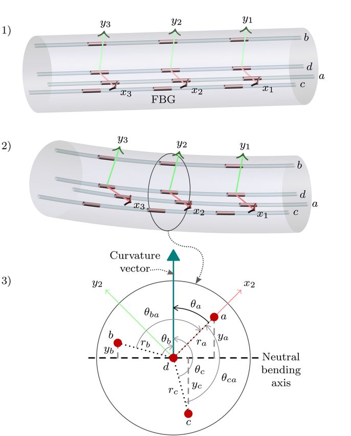
This article has been accepted for publication in a future issue of this journal, but has not been fully edited. Content may change prior to final publication. Citation information: DOI 10.1109/JSEN.2020.2993452, IEEE Sensors
Journal
4
in simulation by Shiyuan et al. [20]. Let γ(s) ∈ R3 be
the position vector of the curve. The frame at s consists of
three orthonormal vectors T(s) ∈ R3 , M1 (s) ∈ R3 , and
M2 (s) ∈ R3 . The derivatives of the position and the frame
with respect to the arc length of the curve are as follows [16]:
dγ(s)
= T(s), (11)
ds
dT(s)
= k1 (s)M1 (s) + k2 (s)M2 (s), (12)
ds
dM1 (s)
= −k1 (s)T(s), (13)
ds
dM2 (s)
= −k2 (s)T(s). (14)
ds
In this study, the parameters k1 (s) ∈ R and k2 (s) ∈ R are
calculated from the values of the curvature vector κ(s) and
θa (s) using the following relation:
k1 (s) = v1 (s) = κ(s)cos(θa (s)), (15)
k2 (s) = v2 (s) = κ(s)sin(θa (s)). (16)
Fig. 4: a) Cross-section and side view of the fibers utilized
This gives values of k1 (s) and k2 (s) at the locations of the
for the experiments. Each fiber has seven cores with eight
FBG sensor sets. The values of k1 (s) and k2 (s) in between the
groups of fiber Bragg grating (FBG) sensors. Two groups of
FBG sensor set locations are estimated using linear interpola-
sensors and the fiber cross-section are shown. A set of sensors
tion. The interpolated values are denoted as ke1 (s) and ke2 (s).
used for the curvature vector calculations consists of four out
The position γ(s) and the frame {M1 (s), M2 (s), T(s)} are
of the seven sensors, as highlighted on the cross-section with
solved using the following matrix form of (11)-(14):
gray discs. b) Photograph of the four-segment catheter used
in the experiments along with an inset that shows the tip.
d Each segment can move independently in the axial direction
X(s) = X(s)A(s), (17)
ds and has two channels that are utilized for an electromagnetic
where, (EM) sensor and a fiber.
T(s) M1 (s) M2 (s) γ(s)
X(s) = , (18) between the reconstruction and the ground truth is calculated
0 0 0 1
using three measures; one measure is the magnitude of the
0 −ke1 (s) −ke2 (s) 1 error in position re ∈ R, the second is the angle between
ke1 (s) 0 0 0 the orientation vector φe ∈ R, and the last measure is the
A(s) = . (19)
ke (s)
2 0 0 0 difference in the rotation angles about the orientation vector
0 0 0 0 θe ∈ R. The error measures are calculated as follows:
The discretized solution to (17) assuming A(s) is held con- re (k) = kr(k) − rgt (k)k (21)
stant between two consecutive values of ke1 (s), and ke2 (s) is vgt (k) · v(k)
φe (k) = cos−1 (22)
given as: kvgt (k)kkv(k)k
θe (k) = kθ(k) − θgt (k)k (23)
X(s + ∆s) = X(s) exp (A(s)∆s) . (20)
where, k ∈ Z≥0 represents the sample of the data; r(k) ∈ R3
The tip pose is given by X(L), where L is the length of the
T is the reconstructed tip position; rgt (k) ∈ R3 is the ground
fiber. The initial position is assumed to be γ(0) = [ 0 0 0 ] and
T T truth of the tip position; v(k) ∈ R3 is the reconstructed tip
the orientation to be M1 (0) = [ 1 0 0 ] , M2 (0) = [ 0 1 0 ] ,
T orientation vector, vgt (k) ∈ R3 is the true orientation vector,
T(0) = [ 0 0 1 ] .
θ(k) ∈ R is the angle of rotation about the reconstructed
The reconstruction technique presented in Section II is
orientation vector and θgt (k) ∈ R is the angle of rotation
empirically validated in the next Section.
about the true orientation vector. Details on the hardware
and software for the experiments are given in Section III-A.
III. E XPERIMENTS Descriptions of the three experiments and the results are given
Three different experiments are conducted to validate the in Sections III-B, III-C and III-D. Registration between the
reconstructed pose using the technique presented in Section II. reference frame of the fibers and the reference frame of the
Particularly, the tip pose is used for validation since the ground truth is conducted for each experiment. A set of points
reconstruction error is the largest there due to the accumulation in each frame is collected and the transformation between the
of error over the length in (20). The difference in tip pose frames is solved using least square estimation [21].
1558-1748 (c) 2020 IEEE. Personal use is permitted, but republication/redistribution requires IEEE permission. See http://www.ieee.org/publications_standards/publications/rights/index.html for more information.
Authorized licensed use limited to: UNIVERSITY OF TWENTE.. Downloaded on May 11,2020 at 06:54:20 UTC from IEEE Xplore. Restrictions apply.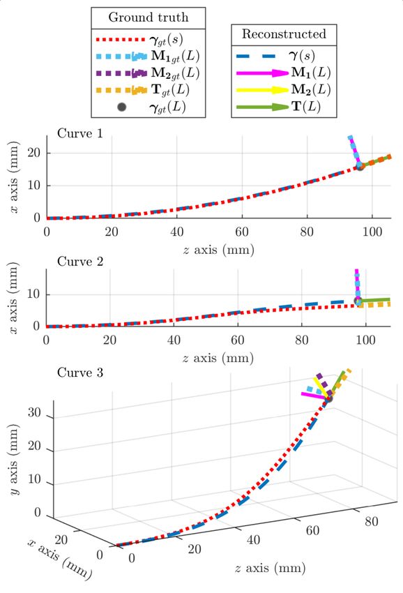
This article has been accepted for publication in a future issue of this journal, but has not been fully edited. Content may change prior to final publication. Citation information: DOI 10.1109/JSEN.2020.2993452, IEEE Sensors
Journal
5
Fan-out boxes unit that is described in Watts et al. [25].
Interrogator
The EM sensor is part of the Aurora System from NDI
Medical (Ontario, Canada), it is 0.3 mm in diameter and
Coupler has five degrees of freedom which include position in three
dimensions, pitch and yaw. The root mean square error of the
Curve 1 EM sensors is 0.70 mm and 0.20◦ in position and orientation,
respectively [26].
Catheter The gelatin phantom is produced to mimic soft brain tissue
Curve 2 Curve 3
Multi-core fiber from 4.5% by weight bovine gelatin [27]. The 3D printed
molds and the actuation unit are designed and built in-house.
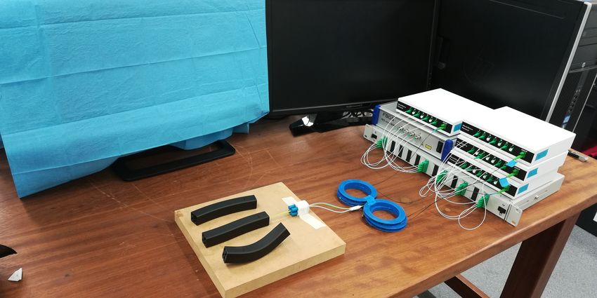
Fig. 5: Setup for Experiment 1. The catheter is sensorized with The software used in the experiments is also developed in-
four multi-core fibers that have fiber Bragg gratings (FBG); house for Ubuntu 16.04.
each catheter segment has one fiber. The experiment utilizes
four multi-core fibers, fan-out boxes, interrogator, coupler,
B. Experiment 1: Static tests
catheter, and three molds.
A four-segment catheter with four fibers is placed in 3D
printed molds and the reconstructed catheter tip pose is com-
A. Setup pared to the tip pose of the mold’s centerline. Table I describes
The hardware for the three experiments consists of a four- the curves that form the centerline of the three molds. Each
segment catheter, four multi-core fibers with eight sets of FBG
sensors, an interrogator, four fan out boxes and a coupler. In
addition, Experiment 1 includes 3D printed molds; Experiment
2 and 3 uses four EM sensors placed at the tip of the four
segments; lastly, Experiment 3 utilizes a gelatin phantom and
an actuation unit. The setup for Experiments 1, 2 and 3 are
shown in Figures 5, 7 and 9, respectively.
The FBG sensors are written using the Draw Tower Grating
technique on all the cores at eight locations on each of the four
fibers [22]. The spectra from a strain-free fiber are shown
in Figure 3. The nominal Bragg wavelength differ between
consecutive FBG sensors by 2.4 nm and the wavelength
range on the four fibers are 1513–1529.8 nm, 1532.2–1549
nm, 1551.4–1568.2 nm, and 1570.6–1587.4 nm. As shown in
Figure 4a, every sensor is 5 mm long and the sensor sets
are 14 mm apart which means the sensorized section of each
fiber is 103 mm. The core and the cladding of the fiber are
composed of fused silica and their refractive indices are 1.454
and 1.444, respectively. The operating temperature range of the
fiber is -20◦ C to 200◦ C [23]. FBGS International NV (Geel,
Belgium) supplied the fibers with FBG sensors, the value of
the gauge factor S = 0.777 in (1), the interrogator (FBG-scan
804D), four fan out boxes and a coupler [24].
The catheter is 2.5 mm in diameter and manufactured with
medical-grade polymer by Xograph Healthcare Ltd. (Glouces-
tershire, United Kingdom). It is illustrated in Figure 4b.
Further information on the catheter manufacturing procedure
and material properties are given in Watts et al. [25]. The shape
of the catheter can be controlled with the relative difference
in the insertion length of the segments. The insertion of each
catheter segment is controlled and executed by the actuation
Fig. 6: The ground truth and the reconstruction plots of the
three curves from one sample in Experiment 1. In the legend,
TABLE I: The curvature and torsion along the arc length of γ(s) ∈ R3 , is the reconstructed curve, where s ∈ R is the arc
the centerline in the molds used for Experiment 1. length parameter. M1 (L) ∈ R3 , M2 (L) ∈ R3 and T(L) ∈ R3
Configuration Curvature (mm−1 ) Torsion (mm−1 ) represent the orientation at the curve’s tip. Similarly, γ gt (s) ∈
Curve 1: Single bend constant: 3.3e−3 constant: 0 R3 , M1gt (L) ∈ R3 , M2gt (L) ∈ R3 , Tgt (L) ∈ R3 are the
Curve 2: Double bend linear: 2.5e−3 to −2.5e−3 constant: 0 analogous values from the ground truth. Lastly, γ gt (L) ∈ R3
Curve 3: Space curve constant: 1.0e−2 constant: 2.2e−2 is the ground truth curve’s tip position.
1558-1748 (c) 2020 IEEE. Personal use is permitted, but republication/redistribution requires IEEE permission. See http://www.ieee.org/publications_standards/publications/rights/index.html for more information.
Authorized licensed use limited to: UNIVERSITY OF TWENTE.. Downloaded on May 11,2020 at 06:54:20 UTC from IEEE Xplore. Restrictions apply.This article has been accepted for publication in a future issue of this journal, but has not been fully edited. Content may change prior to final publication. Citation information: DOI 10.1109/JSEN.2020.2993452, IEEE Sensors
Journal
6
TABLE II: Mean (r̄e , φ̄e , θ̄e ) and standard deviation (σre , σφe , TABLE III: Mean (r̄e , φ̄e ) and standard deviation (σre , σφe )
σθe ) of the error in catheter tip pose from (21), (22) and (23) of the fiber tip pose error according to (21) and (22) over the
over the samples collected for each curve in Experiment 1. samples collected from all four fibers during Experiment 2.
Curve 1 Curve 2 Curve 3 Trial 1 Trial 2 Trial 3
r̄e (σre ) (mm) 0.09 (0.03) 1.45 (0.06) 1.73 (0.05) r̄e (σre ) (mm) 2.20 (1.28) 2.95 (1.88) 2.89 (1.42)
φ̄e (σφe ) (degree) 1.01 (0.09) 0.66 (0.04) 0.37 (0.03) φ̄e (σφe ) (degree) 3.50 (1.38) 3.52 (1.10) 3.37 (1.27)
θ̄e (σθe ) (degree) 0.34 (0.06) 0.32 (0.05) 1.94 (0.06)
is calculated using (21) and (22) where, r(k) is γ(L) and
fiber is reconstructed using (20) and the catheter’s centerline v(k) is T(L) at sample k. The value for rgt (k) and vgt (k)
is calculated as the mean of the reconstructed position and are acquired from the EM sensor measurements. Since the
orientation of the fibers at particular arc lengths. Data from EM sensors have 5 degrees of freedom, the rotation about
Curve 1 are used to solve for the transformation between the the orientation axis is not available. Table III gives the mean
reconstruction frame and the ground truth frame. and standard deviation of the error measures among all the
The reconstruction of the catheter centerline is validated by segments over the duration of every trial. The trajectory of a
the error in the tip pose. The error measures of (21), (22) fiber tip and of the corresponding EM sensor during the first
and (23) are used where v(k) is the axis and θ(k) is the trial is given in Figure 8.
angle from the axis-angle representation of the tip orientation
frame {M1 (L), M2 (L), T(L)} and r(k) is γ(L) at sample k. D. Experiment 3: Dynamic tests conducted in gelatin
Similarly, the ground truth values rgt (k), θgt (k) and vgt (k) The catheter is inserted into a gelatin phantom that mimics
are acquired from the mold’s centerline curve. For this experi- soft brain tissue [25]. The aim is to validate the reconstruction
ment the ground truth values are constant for all samples. The when distributed force is applied along the catheter from the
mean of the error measures and the standard deviation given environment. The catheter is sensorized as in Experiment 2.
in Table II are over all samples. The reconstruction and the Three insertions into the phantom are conducted; in the first
ground truth from a sample of the three curves are shown in insertion the catheter follows a straight path, in the second the
Figure 6. catheter follows a single bend path and finally in the third,
the catheter follows a double bend path. Each insertion is
C. Experiment 2: Dynamic tests conducted in air controlled by an actuation unit as described in Watts et al.
In this experiment, the catheter is moved in air by manually so that the catheter follows the pre-determined path [25]. For
pushing on it from different directions. The objective is to each insertion, data from the FBG sensors in the fibers and
validate the reconstruction by comparing the reconstructed the EM sensors are collected simultaneously.
fiber tip pose to an EM sensor pose. Each of the catheter’s The fiber tip is reconstructed using (20). The error between
four segments is sensorized with a fiber and an EM sensor, the reconstructed fiber tip pose and the EM sensor on the
which is placed at the segment’s tip. The four fibers’ tip same catheter segment is calculated using (21) and (22) where
pose from the reconstruction and the four EM sensors’ pose the variables have the same assignment as in Experiment 2.
are collected over time. The catheter is manually moved for The EM frame and the reconstruction frame are registered
three trials and an additional trial is conducted in order to
solve for the transformation between the EM sensor frame
and the reconstruction frame. The tip pose of each fiber is
reconstructed using (20) and it is compared to the pose of
the EM sensor in the same segment as the fiber. The error
Fan-out boxes
Interrogator
EM Field
Generator Coupler
Catheter
Multi-core fiber
Fig. 8: The trajectory traced by an electromagnetic (EM)
Fig. 7: Setup for Experiment 2. The catheter is sensorized with sensor and the corresponding fiber tip placed in the catheter
fiber Bragg gratings (FBG) inscribed multi-core fibers and during Trial 1. The orientation vectors at selected samples are
electromagnetic (EM) sensors. The hardware utilized consists also shown on the trajectory. k ∈ R represents a sample in
of four multi-core fibers, fan-out boxes, interrogator, coupler, time, r(k) ∈ R3 is the fiber tip position, v(k) ∈ R3 is the
four-segment catheter, four electromagnetic (EM) sensors and fiber tip orientation vector. rgt (k) ∈ R3 and vgt (k) ∈ R3 are
EM field generator. the position and orientation from the EM sensor, respectively.
1558-1748 (c) 2020 IEEE. Personal use is permitted, but republication/redistribution requires IEEE permission. See http://www.ieee.org/publications_standards/publications/rights/index.html for more information.
Authorized licensed use limited to: UNIVERSITY OF TWENTE.. Downloaded on May 11,2020 at 06:54:20 UTC from IEEE Xplore. Restrictions apply.This article has been accepted for publication in a future issue of this journal, but has not been fully edited. Content may change prior to final publication. Citation information: DOI 10.1109/JSEN.2020.2993452, IEEE Sensors
Journal
7
that they can be detached and reused. Thus, the fibers are free
Actuation within the channel and can move relative to the catheter. The
Unit error due to fiber motion may be reduced by incorporating a
Gelatin
mechanics model of the catheter in the pose measurement.
V. C ONCLUSION AND F UTURE W ORK
Catheter A technique for acquiring the pose of a flexible instrument
from FBG measurements is presented in the paper. The
Trocar EM Field
Generator measurements from the FBG sensors are first converted to
strain and then the curvature vectors are calculated at the
Fig. 9: Setup for Experiment 3. The catheter followed a single locations on the fiber with co-located FBG sensors. The
bend path. It is sensorized with multi-core fibers that have curvature calculation uses the strain values from the sensors
fiber Bragg gratings (FBG) and electromagnetic (EM) sensors. and the theory of bending mechanics. Once the curvature is
The experiment utilizes hardware from Experiment 2 and in calculated, the fiber is reconstructed using Bishop Frames.
addition requires an actuation unit, trocar to hold the catheter The reconstruction provides the pose of the fiber along its
and gelatin phantom. arc length and the tip pose is validated in two dynamics
experiments. The reconstruction of four fibers is utilized to
deduce an instrument’s tip pose which is validated in static
using data from a trial that constituted of manually moving the experiments. The results from all the experiments show that
catheter in air. Figure 10 shows the plot of a catheter segment’s the mean error in position is less than 4.69 mm and mean
tip trajectory during the second insertion which consisted of error in orientation is less than 6.48 degrees. Thus, acquiring
a single bend path. The mean and standard deviation of the the pose of a flexible instrument is feasible with FBG sensors
error measures for the three insertions are given in Table IV. in multi-core fiber. In future work, temperature sensing and
temperature compensation using FBG sensors in multi-core
IV. D ISCUSSION fiber will be studied.
In the static experiments, the difference in error between
this study and Khan et al. is possibly due to the different FBG
inscription method utilized for the sensors. In this study Draw
Tower Grating (DTG) technique is used whereas Khan et al.
used a Phase Mask (PM) technique [13]. The DTG technique
produced sensors with reflectivity of 3% of the input light
whereas the PM technique produced sensors with reflectivity
of at least 30%. The higher reflectivity of the sensors inscribed
with PM technique could led to more accurate detection
of the Bragg wavelength, which would result in a lower
reconstruction error. However, for the PM technique the fiber
coating is removed before inscription, which made the fiber
very fragile and unsuitable for dynamic experiments with Fig. 10: The trajectory during insertion 2 of the electromag-
gelatine or soft tissue. In the DTG technique the sensors are netic (EM) sensor and the fiber tip from one of the catheter’s
inscribed just after the fiber is drawn and before the coating is segments. k ∈ R represents a sample in time, r(k) ∈ R3 is the
applied [28]. Since the original coating of the fiber remained fiber tip position, and v(k) ∈ R3 is the fiber tip orientation
intact the resulting fiber had high breakage strength, which is vector. rgt (k) ∈ R3 and vgt (k) ∈ R3 are the position and
necessary for dynamic experiments. For this reason, sensors orientation from the EM sensors, respectively.
inscribed with DTG technique are utilized in this study.
In the dynamic experiments, the error may be caused by the
fiber’s motion relative to the catheter. The fibers are attached ACKNOWLEDGMENTS
to the segments at a single point near the catheter base, so
The authors would like to thank Dr. Riccardo Secoli and
Ms. Eloise Matheson for their help with Experiment 3. In
TABLE IV: Mean (r̄e , φ̄e ) and standard deviation (σre , σφe ) of addition, the authors appreciate the valuable feedback on the
the fiber tip pose error according to (21) and (22) for the three manuscript from Dr. Venkat Kalpathy Venkiteswaran and Mr.
insertions in Experiment 3. The mean and standard deviation Jakub Sikorski.
is over all the tip pose collected from the four fibers and EM
sensors during each insertion. R EFERENCES
Insertion 1 Insertion 2 Insertion 3 [1] D. Tosi, E. Schena, C. Molardi, and S. Korganbayev, “Fiber optic
r̄e (σre ) (mm) 1.54 (1.34) 4.35 (2.17) 4.69 (2.81) sensors for sub-centimeter spatially resolved measurements: Review and
biomedical applications,” Optical Fiber Technology, vol. 43, pp. 6 – 19,
φ̄e (σφe ) (degree) 2.85 (2.11) 6.48 (3.18) 3.49 (2.51) 2018.
1558-1748 (c) 2020 IEEE. Personal use is permitted, but republication/redistribution requires IEEE permission. See http://www.ieee.org/publications_standards/publications/rights/index.html for more information.
Authorized licensed use limited to: UNIVERSITY OF TWENTE.. Downloaded on May 11,2020 at 06:54:20 UTC from IEEE Xplore. Restrictions apply.This article has been accepted for publication in a future issue of this journal, but has not been fully edited. Content may change prior to final publication. Citation information: DOI 10.1109/JSEN.2020.2993452, IEEE Sensors
Journal
8
[2] C. Shi, X. Luo, P. Qi, T. Li, S. Song, Z. Najdovski, T. Fukuda, and [24] Manual ‘ILLumiSense’ software, Version 2.3, FBGS International, Bell
H. Ren, “Shape sensing techniques for continuum robots in minimally Telephonelaan 2H, Geel Belgium, 2014.
invasive surgery: A survey,” IEEE Transactions on Biomedical Engi- [25] T. Watts, R. Secoli, and F. Rodriguez y Baena, “A mechanics-based
neering, vol. 64, no. 8, pp. 1665–1678, 2017. model for 3-D steering of programmable bevel-tip needles,” IEEE
[3] R. Reilink, S. Stramigioli, and S. Misra, “Pose reconstruction of flexible Transactions on Robotics, vol. 35, no. 2, pp. 371–386, 2019.
instruments from endoscopic images using markers,” in 2012 IEEE [26] NDI Medical, “Aurora-Medical,” Sept 2013. [Online].
International Conference on Robotics and Automation, May 2012, pp. https://www.ndigital.com/medical/products/aurora/ [Accessed: January
2938–2943. 7, 2020].
[4] P. Cabras, F. Nageotte, P. Zanne, and C. Doignon, “An adaptive and [27] A. Leibinger, A. E. Forte, Z. Tan, M. J. Oldfield, F. Beyrau, D. Dini, and
fully automatic method for estimating the 3D position of bendable F.Rodriguez y Baena, “Soft tissue phantoms for realistic needle insertion:
instruments using endoscopic images,” The International Journal of A comparative study,” Annals of Biomedical Engineering, vol. 44, no. 8,
Medical Robotics + Computer Assisted Surgery : MRCAS, vol. 13, no. 7, pp. 2442–2452, 2016.
pp. 1–14, 2017. [28] FBGS International NV, “DTG & FSG Technology,” Jan 2019. [On-
[5] A. M. Franz, T. Haidegger, W. Birkfellner, K. Cleary, T. Peters, and line]. Available: https://fbgs.com/technology/dtg-fsg-technology/ [Ac-
L. Maier-Hein, “Electromagnetic tracking in medicine-a review of cessed: January 7, 2020].
technology, validation, and applications,” IEEE Transactions on Medical
Imaging, vol. 33, no. 8, pp. 1702–1725, 2014.
[6] F. Taffoni, D. Formica, P. Saccomandi, G. Di Pino, and E. Schena,
“Optical fiber-based MR-compatible sensors for medical applications:
An overview,” Sensors, vol. 13, no. 10, pp. 14 105–14 120, 2013.
[7] B. Lee, “Review of the present status of optical fiber sensors. optical
fiber technology 9, 57-79,” Optical Fiber Technology, vol. 9, no. 2, pp.
57–79, 2003.
[8] S. Sareh, Y. Noh, M. Li, T. Ranzani, H. Liu, and K. Althoefer,
“Macrobend optical sensing for pose measurement in soft robot arms,”
Smart Materials and Structures, vol. 24, pp. 1–14, 2015.
[9] J. P. Moore and M. D. Rogge, “Shape sensing using multi-core fiber
optic cable and parametric curve solutions,” Opt. Express, vol. 20, no. 3,
pp. 2967–2973, 2012.
[10] Y. Xinhua, W. Mingjun, and C. Xiaomin, “Deformation sensing of
colonoscope on FBG sensor net,” TELKOMNIKA : Indonesian Journal
of Electrical Engineering, vol. 10, no. 8, pp. 2253–2260, 2012.
[11] Y. Park, S. Elayaperumal, B. Daniel, S. C. Ryu, M. Shin, J. Savall, R. J.
Black, B. Moslehi, and M. R. Cutkosky, “Real-time estimation of 3-D
needle shape and deflection for MRI-guided interventions,” IEEE/ASME
Transactions on Mechatronics, vol. 15, no. 6, pp. 906–915, 2010.
[12] R. J. Roesthuis, M. Kemp, J. J. van den Dobbelsteen, and S. Misra,
“Three-dimensional needle shape reconstruction using an array of fiber
bragg grating sensors,” IEEE/ASME Transactions on Mechatronics,
vol. 19, no. 4, pp. 1115–1126, 2014.
[13] F. Khan, A. Denasi, D. Barrera, J. Madrigal, S. Sales, and S. Misra,
“Multi-core optical fibers with bragg gratings as shape sensor for flexible
medical instruments,” IEEE Sensors, vol. 19, no. 14, pp. 5878–5884,
2019.
[14] K. Henken, D. van Gerwen, J. Dankelman, and J. Dobbelsteen, “Ac-
curacy of needle position measurements using fiber bragg gratings,”
Minimally Invasive Therapy & Allied Technologies, vol. 21, no. 6, pp.
408–414, 2012.
[15] A. Gray, Modern Differential Geometry of Curves and Surfaces with
Mathematica. Boca Raton, Florida, United States of America: Chapman
& Hall/CRC, 2006.
[16] R. L. Bishop, “There is more than one way to frame a curve,” The
American Mathematical Monthly, vol. 82, no. 3, pp. 246–251, 1975.
[17] K. O. Hill and G. Meltz, “Fiber Bragg grating technology fundamentals
and overview,” Journal of Lightwave Technology, vol. 15, no. 8, pp.
1263–1276, 1997.
[18] J. Van Roosbroeck, C. Chojetzki, J. Vlekken, E. Voet, and M. Voet,
“A new methodology for fiber optic strain gage measurements and its
characterization,” in Proceedings of the SENSOR+TEST Conferences,
vol. OPTO 2 - Optical Fiber Sensors, pp.59 - 64, Nürnberg, Germany,
May 2009.
[19] R. C. Hibbeler, Mechanics of materials, 8th ed. Upper Saddle River,
New Jersey, United States: Pearson Prentice Hall, 2011.
[20] Z. Shiyuan, J. Cui, C. Yang, and J. Tan, “Parallel transport frame for
fiber shape sensing,” IEEE Photonics Journal, vol. 10, no. 1, pp. 1–13,
2018.
[21] S. Umeyama, “Least-squares estimation of transformation parameters
between two point patterns,” IEEE Transactions on Pattern Analysis
and Machine Intelligence, vol. 13, no. 4, pp. 376–380, 1991.
[22] B. Van Hoe, J. Van Roosbroeck, C. Voigtlnder, J. Vlekken, and
E. Lindner, “Distributed strain and curvature measurements based on
tailored draw tower gratings,” in IEEE Avionics and Vehicle Fiber-Optics
and Photonics Conference (AVFOP), pp.285-286, California, USA, Oct
2016.
[23] FBGS International NV, “Draw Tower Gratings (DTG),” Jan 2019.
[Online]. Available: https://fbgs.com/components/draw-tower-gratings-
dtgs/ [Accessed: January 7, 2020].
1558-1748 (c) 2020 IEEE. Personal use is permitted, but republication/redistribution requires IEEE permission. See http://www.ieee.org/publications_standards/publications/rights/index.html for more information.
Authorized licensed use limited to: UNIVERSITY OF TWENTE.. Downloaded on May 11,2020 at 06:54:20 UTC from IEEE Xplore. Restrictions apply.You can also read